TítuloParallel construction of wavelet trees on multicore architectures

Texto completo

(1)Knowledge and Information Systems manuscript No. (will be inserted by the editor). Parallel Construction of Wavelet Trees on Multicore Architectures José Fuentes-Sepúlveda · Erick Elejalde · Leo Ferres · Diego Seco. Abstract The wavelet tree has become a very useful data structure to efficiently represent and query large volumes of data in many different domains, from bioinformatics to geographic information systems. One problem with wavelet trees is their construction time. In this paper, we introduce two algorithms that reduce the time complexity of a wavelet tree’s construction by taking advantage of nowadays ubiquitous multicore machines. Our first algorithm constructs all the levels of the wavelet in parallel in O(n) time and O(n lg σ + σ lg n) bits of working space, where n is the size of the input sequence and σ is the size of the alphabet. Our second algorithm constructs the wavelet tree in a domain-decomposition fashion, using our first algorithm in each segment, reaching O(lg n) time and O(n lg σ + pσ lg n/ lg σ) bits of extra space, where p is the number of available cores. Both algorithms are practical and report good speedup for large real datasets. Keywords Succinct Data Structure · Wavelet Tree Construction · Multicore · Parallel Algorithm A previous version of this paper appeared in the 13th International Symposium on Experimental Algorithms (SEA 2014)[15]. This work was supported in part by the European Union’s Horizon 2020 research and innovation programme under the Marie Sklodowska-Curie grant agreement No 690941 and the doctoral scholarships of CONICYT No 21120974 and 63130228 (first and second authors, respectively). We also would like to thank Roberto Ası́n for making his multicore computers, Mastropiero and Günther Frager, available to us. This is an Author’s Original Manuscript of an article whose final and definitive form, the Version of Record, has been published in Knowledge and Information Systems [copyright Springer], available online at: http://dx.doi.org/10.1007/s10115-016-1000-6. José Fuentes-Sepúlveda · Erick Elejalde · Diego Seco Department of Computer Science, Universidad de Concepción, Chile. E-mail: {jfuentess,eelejalde,dseco}@udec.cl Leo Ferres Faculty of Engineering, Universidad del Desarrollo, Chile E-mail: [email protected] Corresponding authors: José Fuentes-Sepúlveda · Leo Ferres.

(2) 2. J. Fuentes-Sepúlveda, E. Elejalde, L. Ferres, D. Seco. 1 Introduction and motivation After their introduction in the mid-2000s, multicore computers –computers with more than one processing unit (called cores) and shared memory– have become pervasive. In fact, nowadays it is difficult to find a single-processor desktop, let alone a high-end server. The argument in favor of multicore systems is simple: thermodynamic and material considerations prevent chip manufacturers from ever increasing clock rates. Since 2005, clock frequencies have stagnated at around 3.75GHz for commodity computers, and even in 2015, 4GHz computers are still high-end (the Intel Core i7-4790K is a prime example). Thus, the next step in performance is to take advantage of the processing power of multicore computers. In order to do this, algorithms and data structures will have to be modified to make them behave well in these parallel architectures. At the same time, the amount of data to be processed has become large enough that the ability to maintain it close to the processor is vital. This, in turn, has generated a keen interest in succinct data structures, which besides reducing storage requirements, may also reduce the number of memory transfers, the energy consumption, and can be used in low-capacity devices such as smartphones. One such structure that has benefited from thorough research is the wavelet tree [18], henceforth wtree. Although the wtree was originally devised as a data structure for encoding a reordering of the elements of a sequence [18, 14], it has now been successfully used in many critical applications such as indexing documents [33], in processing grids [25] and sets of rectangles [4], to name but a few. Two excellent surveys have been written about this data structure [24, 22], and we refer the readers to them for more application examples and details. These succinct data structures, however, are generally quite expensive (in time) to build, particularly as the size of the alphabet and the size of the input increase, as is the case nowadays with the so-called “big data” revolution. We believe parallel computing is a good tool for speeding up the processing of succinct data structures. Unfortunately, (practical) parallel computing suffers from several drawbacks that make these high-performant algorithms difficult to come by: maintaing thread independence while communicating results, keeping clear of “thrashing” the memory hierarchy are two such problems. Thus, a sizeable contribution to the state-of-the-art would involve designing algorithms with good theoretical running times that are also practical in modern commodity architectures with more than one core, which would also help speed up processing of the target data structures in distributed systems: if one node is faster, the whole cluster would be faster as well. Motivating example. Perhaps one of the prominent areas of research in the last few years has been the analysis of genomic data [28, 30, 26]. In combination with the Burrows-Wheeler transform [5], the wtree has been used to construct compressed full-text indexes (the FM-index [12, 13]) over DNA sequences. The structure supports efficient algorithms for important problems in bioinformatics such as the identification of patterns (like the mutations that are known to cause some diseases) or the alignment of short DNA sequences, known as reads (which is a fundamental step to reconstruct a genome), all this without decompressing the data. The cost of DNA sequencing has plummeted in the last few years thanks to next-generation sequencing technologies [34]. In addition, these technologies are.

(3) Parallel Construction of Wavelet Trees on Multicore Architectures. 3. also much faster. For example, in 2005, a single sequencing run could generate at most one gigabase of data. Meanwhile, in 2014, a single sequencing run could generate up to 1.8 terabases of data [20]. These two factors have drastically increased the amount of genomic data to be processed. Therefore, full-text indexes based on wtrees need to be updated periodically. These updates do not modify the already indexed data but add new sequences. This process is not trivial because the Burrows-Wheeler transform is a reorganization of the whole sequence in order to make it more compressible. In order to support these updates there are two options: the use of fully dynamic wtrees or the periodic reconstruction of the wtree (a solution used in other domains such as Web search engines). Dynamic versions of wtrees are quite slow in both update and rank/select operations (see Section 3.2 of [22]). The other option is the usage of a static wtree and a buffer (which stores the updates since the last reconstruction of the static index). To support queries, both the static wtree and the buffer are used. When the buffer is full, the static wtree is reconstructed considering the symbols on the buffer, which is emptied after that. Thus, improving the construction time of static wtrees becomes critical, for example, to provide solutions in this kind of dynamic domain in which queries are much more frequent than updates. In this paper, we propose two parallel algorithms for the most expensive operation on wtrees: its construction. The first algorithm, pwt, has O(n) time complexity and uses O(n lg σ + σ lg n) bits of space1 , including the space of the final wtree and excluding the input, where σ is the size of the alphabet. The second algorithm, dd, is an improved version of the dd algorithm presented on [15]. This new version has O(lg n) time complexity and uses O(n lg σ + pσ lg n/ lg σ) bits of space, using p threads (see Sect. 3). The pwt algorithm improves the O(n) memory consumption in [29]. Meanwhile, the new dd algorithm improves the O(n) time complexity of our previous work [15] and the time complexity of [29] by a factor of O(lg σ). We report experiments that demonstrate the algorithms to be not only theoretically good, but also practical for large datasets on commodity architectures, achieving good speedup (Sect. 4). As far as we can tell, we use the largest datasets to-date and our algorithms are faster for most use cases than the state-of-the-art [29].. 2 Background and related work 2.1 Dynamic multithreading model Dynamic multithreading (DYM) [10, Chapter 27] is a model of parallel computation which is faithful to several industry standards such as Intel’s CilkPlus (cilkplus.org), OpenMP Tasks (openmp.org/wp), and Threading Building Blocks (threadingbuildingblocks.org). Besides its mathematical rigour, it is precisely this adoption by many high-end compiler vendors that make the model so appealing for practical parallel algorithms. In the Dynamic multithreading model, a multithreaded computation is defined as a directed acyclic graph (DAG) G = (V, E), where the set of vertices V are instructions and (u, v) ∈ E are dependencies between the instructions; whereby 1. We use lg x = log2 x..

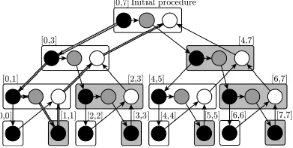
(4) 4. J. Fuentes-Sepúlveda, E. Elejalde, L. Ferres, D. Seco. in this case, u must be executed before v.2 In order to signal parallel execution, we augment sequential pseudocode with three keywords, spawn, sync and parfor. The spawn keyword signals that the procedure call that it precedes may be executed in parallel with the next instruction in the instance that executes the spawn. In turn, the sync keyword signals that all spawned procedures must finish before proceeding with the next instruction in the stream. Finally, parfor is simply “syntactic sugar” for spawn’ing and sync’ing ranges of a loop iteration. If a stream of instructions does not contain one of the above keywords, or a return (which implicitly sync’s) from a procedure, we group these instruction into a single strand. The parfor keyword, which we use repeatedly here, is implemented by halving the range of loop iterations, spawn’ing one half and using the current procedure to process the other half recursively until reaching one iteration per range. After that, the iterations are executed in parallel. This implementation adds an overhead to the parallel algorithm bounded above by the logarithm of the number of loop iterations. For example, Algorithm 1 represents a parallel algorithm using parfor and Figure 1 shows its multithreaded computation. In the figure, each circle represents one strand and each rounded rectangle represents strands that belong to the same procedure call. The algorithm starts on the initial procedure call with the entire range [0, 7]. The first half of the range is spawned (black circle in the initial call) and the second half is processed by the same procedure (gray circle of the initial call). This divide-and-conquer strategy is repeated until reaching strands with one iteration of the loop (black circles on the bottom of the figure). Once an iteration is finished, the corresponding strand syncs to its calling procedure (white circles), until reaching the final strand (white circle of the initial call). For more examples of the usage of the DYM model, see [10, Chapter 27]. Strands are scheduled onto cores using a work-stealing scheduler, which does the load-balancing of the computations. Work-stealing schedulers have been proved to be a factor of 2 away from optimal performance [3]. A : array of 8 numbers parfor i = 0 to 7 do A[i] = 0 return Algorithm 1: Example of a parallel algorithm using the parfor keyword. In parallel, the algorithm initializes all the elements of the array A with 0.. Fig. 1: Example of a multithreaded computation on the Dynamic Multithreading Model. It corresponds to the Directed Acyclic Graph representation of the Algorithm 1. Vertices represent strands and edges represent dependences. To measure the efficiency of our parallel wavelet tree algorithms, we use three metrics: the work, the span and speedup. In accordance to the parallel literature, we will subscript running times by p, so Tp is the running time of an algorithm on p cores. The work is the total running time taken by all strands when executing 2 Notice that the RAM model is a subset of the DYM model where the outdegree of every vertex v ∈ V is ≤ 1..

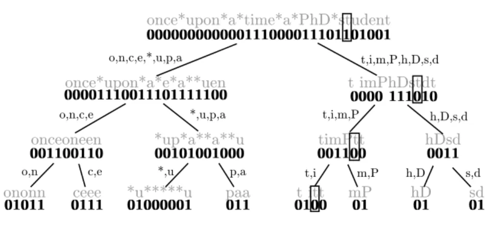
(5) Parallel Construction of Wavelet Trees on Multicore Architectures. 5. on a single core (i.e., T1 ), while the span, denoted as T∞ , is the critical path (the longest path) of G. In Figure 1, assuming that each strand takes unit time, the work is 29 time units and the span is 8 time units (this is represented in the figure with thicker edges). In this paper, we are interested in speeding up wavelet tree manipulation and improving the lower bounds of this speedup. To measure this, we will define speedup as T1 /TP = O(p), where linear speedup T1 /Tp = Θ(p), is the goal and the theoretical upper bound. We also define parallelism as the ratio T1 /T∞ , the theoretical maximum number of cores for which it is possible to achieve linear speedup.. 2.2 Wavelet trees A wavelet tree (wtree) is a data structure that maintains a sequence of n symbols S = s1 , s2 , . . . , sn over an alphabet Σ = [1..σ] under the following operations: access(S, i), which returns the symbol at position i in S; rank c (S, i), which counts the times symbol c appears up to position i in S; and select c (S, j), which returns the position in S of the j-th appearance of symbol c. Storage space of wtrees can be bounded by different measures of the entropy of the underlying data, thus enabling compression. In addition, they can be implemented efficiently [7] and perform well in practice. The wtree is a balanced binary tree. We identify the two children of a node as left and right. Each node represents a range R ⊆ [1, σ] of the alphabet Σ, its left child represents a subset Rl , which corresponds with the first half of R, and its right child a subset Rr , which corresponds with the second half. Every node virtually represents a subsequence S ′ of S composed of symbols whose value lies in R. This subsequence is stored as a bitmap in which a 0 bit means that position i belongs to Rl and a 1 bit means that it belongs to Rr . At its simplest, a wtree requires n⌈lg σ⌉ + o(n lg σ) bits for the data, plus O(σ lg n) bits to store the topology of the tree (considering one pointer per node), and supports aforementioned queries in O(lg σ) time by traversing the tree using O(1)-time rank/select operations on bitmaps [27]. A simple recursive construction algorithm takes O(n lg σ) time. As mentioned before, the space required by the structure can be reduced: the data can be compressed and stored in space bounded by its entropy (via compressed encodings of bitmaps and modifications on the shape of the tree), and the O(σ lg n) bits of the topology can be removed, effectively using one pointer per level of the tree [7], which is important for large alphabets. We focus on construction using a pointer per level because, even though it adds some running time costs, it is more suitable for big data. This notwithstanding, it is trivial to apply the technique to the one-pointer-per-node construction case, and our results can be readily extended to other encodings and tree shapes. Figure 2 shows an example of two wtree representations for the sequence S = “once upon a time a P hD student”. Figure 2a shows the one-pointer-pernode representation, while Figure 2b shows the one-pointer-per-level representation. In our algorithms, we implemented the one-pointer-per-level representation; however, for clarity, we use the one-pointer-per-node representation to exemplify. In both representations we highlighted the traversal performed by the operation access(S, 24). To answer it, a top-down traversal of the wtree is performed: if a bit 0 is found, we visit the left branch; if a 1, the right branch is chosen. In.

(6) 6. J. Fuentes-Sepúlveda, E. Elejalde, L. Ferres, D. Seco. (a) Representation of a wtree using one pointer per node and its associated bitmap. The subsequences of S in the nodes (gray font) and the subsets of Σ in the edges are drawn for illustration purposes.. (b) Representation of a wtree using one pointer per level and its associtaed n-bit bitmap. It can simulate the nagivation on the tree by using the rank operation over the bitmaps.. Fig. 2: A wtree for the sequence S =“once upon a time a PhD student” and the contiguous alphabet Σ = {o,n,c,e,‘ ’,u,p,a,t,i,m,P,h,D,s,d}. We draw spaces using stars.. the first representation, the query works as follows: Let curr be the root, Bcurr be the bitmap of the current node, i = 24 be the index of interest, R be the range [0, σ − 1] = [0, 15] and rank c (Bcurr , i) be the number of c-bits up to position i in Bcurr . At the beginning, we inspect the bit Bcurr [i]. Since the bit is 1, we recompute i = rank 1 (Bcurr , i) − 1 = 7, change curr to be the right child of curr and halve R = [8, 15]. Then, we repeat the process. Since Bcurr [i] = 0, i = rank 0 (Bcurr , i) − 1 = 4, curr is updated to be the left child of curr and R = [8, 11]. Now, Bcurr [i] = 0, i = rank 0 (Bcurr , i) − 1 = 2, curr is changed to be the left child of curr and R = [8, 9]. Finally, in the last level, Bcurr [i] = 0, so the range R = [8, 8] and the answer for access (S, 24) is Σ[8] =‘ t ’. rank c (S, i) and select c (S, i) perform similar traversals to access(S, i). For a more detailed explanation of wtree operations, see [24]. For the one-pointer-per-level representation, the procedure is similar, with the exception that the traversal of the tree must be simulated with rank operations over the bitmaps [7]. Practical implementations of wtrees can be found in Libcds [6] and Sdsl [16]. Libcds implements a recursive construction algorithm that works by halving Σ into binary sub-trees whose left children are all 0s and right children are all 1s, until.

(7) Parallel Construction of Wavelet Trees on Multicore Architectures. 7. 1s and 0s mean only one symbol in Σ. Sdsl implements an algorithm based in the idea of counting sort that is more efficient in memory. The algorithm counts the number of bits that will be placed in each node of the wtree, computing the position of each symbol in each level of the wtree, which avoids maintaining a permutation of the input. Both libraries are the best current sequential implementations available, without considering space efficient construction algorithms [9, 31]. As of late, some work has been done in parallel processing of wtrees. In [1], the authors explore the use of wavelet trees in web search engines. They assume a distributed memory model and propose partition techniques to balance the workload of processing wtrees. Note that our work is complementary to theirs, as each node in their distributed system can be assumed to be a multicore computer that can benefit from our algorithms. In [21], the authors explore the use of SIMD instructions to improve the performance of wtrees and other string algorithms [11]. This set of instructions can be considered as low-level parallelism, since they use instructions in modern processors that work by joining registers for some integer computation, dealing with 128-bit integers at a time. We can also benefit from their work as it may improve the performance of the sequential parts of our algorithms. However, we leave this optimization for future work. In [15], we introduced the first two parallel algorithms for wtree construction: pwt and dd, both with O(n) time complexity. The details of pwt and an improvement of dd are given on Sections 3.1 and 3.2, respectively. Based on [15], Shun [29] introduces two new parallel algorithms. The first algorithm, called levelWT, constructs the wtree level-by-level. In each of the ⌈lg σ⌉ levels, the algorithm uses a parallel prefix sum algorithm to compute the position of the bits, constructing the nodes and their bitmaps in parallel with O(n) work and O(lg n) span, which results in O(n lg σ) work and O(lg n lg σ) span. The second algorithm, called sortWT, constructs all levels in parallel, similar to our original pwt, instead of one-by-one. For a level l, the sortWT algorithm applies a parallel stable integer sorting using the l most significant bits of each symbol as the key. With the sorted input sequence, the algorithm fills the corresponding bitarrays in parallel, using parallel prefix sum and filter algorithms to compute the position of the bits. The total work of the sortWT algorithm is O(Wsort lg σ), where Wsort is the work incurred by sorting, and O(Ssort + lg n) is the span, and where, in turn, Ssort corresponds to the span of the sorting algorithm and the lg n component is the span of the prefix sum and filter algorithms. The author also discusses a variation of the sortWT algorithm, reaching O(n lg σ) work and O(lg n lg σ) span. In practice, the levelWT algorithm shows better performance. Compared to our previous algorithms, the levelWT and sortWT algorithms can scale beyond O(lg σ) cores. However, both also need to duplicate and modify the input sequence, resulting in an increase in memory usage, requiring O(n lg n) bits of extra space.. 2.3 Problem statement The wtree is a versatile data structure that uses n lg σ + o(n lg σ) bits of space and supports several queries (such as access, rank and select) in O(lg σ) time, for a sequence of n symbols over an alphabet Σ of size σ. The wtree can be constructed in O(n lg σ) time, which may be prohibitive for large sequences. Therefore, in this work, we reduce the time complexity of the most time-consuming operation of.

(8) 8. J. Fuentes-Sepúlveda, E. Elejalde, L. Ferres, D. Seco. wtree, its construction, on multicore architectures. Given a multicore machine with p available cores, we propose the design and implementation of parallel algorithms to the construction of wtree. The proposed algorithms scale with p, achieving good practical speedups and extra-memory usage.. 3 Multicore wavelet tree We focus on binary wavelet trees where the symbols in Σ are contiguous in [1, σ]. If they are not contiguous, a bitmap is used to remap the sequence to a contiguous alphabet [7]. Under these restrictions, the wtree is a balanced binary tree with ⌈lg σ⌉ levels. In this section we build the representation of wtrees that removes the O(σ lg n) bits of the topology. Hence, when we refer to a node, this is a conceptual node that does not exist in the actual implementation of the data structure. In what follows, two iterative construction algorithms are introduced that capitalize on the idea that any level of the wtree can be built independently from the others. Unlike in classical wtree construction, when building a level we cannot assume that any previous step is providing us with the correct permutation of the elements of S. Instead, we compute the node at level i for each symbol of the original sequence. More formally, Proposition 1 Given a symbol s ∈ S and a level i, 0 ≤ i < l = ⌈lg σ⌉, of a wtree, the node at which s is represented at level i can be computed as s ≫ l − i. In other words, if the symbols of Σ are contiguous, then the i most significant bits of the symbol s give us its corresponding node at level i. In the word-RAM model with word size Ω(lg n), this computation takes O(1) time. Since the wordRAM model is a subset of the DYM model2 , the following corollary holds: Corollary 1 The node at which a symbol s is represented at level i can be computed in O(1) time.. 3.1 Per-level parallel algorithm Our first algorithm, called pwt, is shown in Algorithm 2 (the sequential version can be obtained by replacing parfor instructions with sequential for instructions). The algorithm takes as input a sequence of symbols S, the length n of S, and the length of the alphabet, σ (see Sect. 2.2). The output is a wtree W T that represents S. We denote the ith level of W T as W T [i], ∀i, 0 ≤ i < ⌈lg σ⌉. The outer loop (line 2) iterates in parallel over ⌈lg σ⌉ levels. Lines 3 to 14 scan each level performing the following tasks: the first step (lines 3 and 4) initializes the bitmap B of the ith level and initializes an array of integers C. The array C will be used to count the number of bits in each node of the wtree at level i, using counting sort. The second step (lines 5 and 6) computes the size of each node in the ith level performing a linear-time sweep over S. For each symbol in S, the algorithm computes the corresponding node for alphabet range at the current level. The expression S[j]/2⌈lg σ⌉−i in line 6 shows an equivalent representation of the idea in Proposition 1. The third step performs a parallel prefix sum algorithm [19] over the array C, obtaining the offset of each node. Once the offset of the nodes is known,.

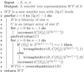
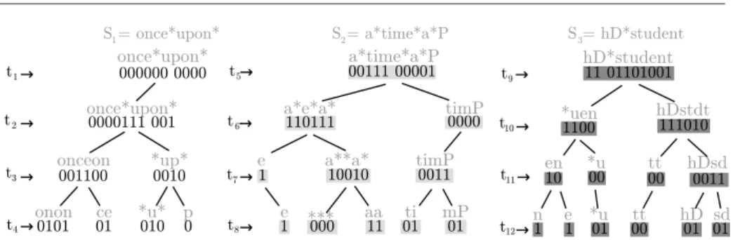
(9) Parallel Construction of Wavelet Trees on Multicore Architectures. 9. Input : S, n, σ Output: A wavelet tree representation W T of S 1 2 3 4 5 6 7 8 9 10 11 12 13 14 15. W T is a new wavelet tree with ⌈lg σ⌉ levels parfor i = 0 to ⌈lg σ⌉ − 1 do B is a bitarray of size n C is an integer array of size 2i for j = 0 to n − 1 do increment(C[S[j]/2⌈lg σ⌉−i ]) parPrefixSum(C ) for j = 0 to n − 1 do if (S[j] & 2⌈lg σ⌉−i−1 ) == 1 then bitmapSetBit(B, C[S[j]/2⌈lg σ⌉−i ], 1) else bitmapSetBit(B, C[S[j]/2⌈lg σ⌉−i ], 0) increment(C[S[j]/2⌈lg σ⌉−i ]) W T [i] = createRankSelect(B ) return W T. Algorithm 2: Per-level parallel algorithm (pwt). the algorithm constructs the corresponding bitarray B, sequentially scanning S (lines 8 to 13). For each symbol in S, the algorithm computes the corresponding node and whether the symbol belongs to either the first or second half of Σ for that node. The corresponding bit is set using bitmapSetBit at position C[S[j]/2⌈lg σ⌉−i ]. Line 14 creates the rank/select structures of the bitmap B of the ith level.. Fig. 3: Snapshot of an execution of the algorithm pwt for the sequence introduced in Figure 2. In the snapshot, thread t1 is writing the first bit of the symbol S[10] =‘ a ’ at level 0, thread t2 is writing the second bit of S[15] =‘ e ’ at level 1, thread t3 is writing the third bit of S[19] =‘ P ’ at level 2 and thread t4 is writing the fourth bit of S[26] =‘ d ’ at level 3. Black areas represent bits associated to unprocessed symbols..

(10) 10. J. Fuentes-Sepúlveda, E. Elejalde, L. Ferres, D. Seco Input : S, n, σ, k Output: A wavelet tree representation W T of S. 1 2 3 4 5 6 7 8 9 10 11 12. W T is a new tree with ⌈lg σ⌉ levels B is an array of ⌈lg σ⌉ bitarrays of size n pB is a bidimensional array of bitarrays of dimensions k × ⌈lg σ⌉ G, L are tridimensional arrays of integers of dimensions k × ⌈lg σ⌉ × 2level parfor i = 0 to k − 1 do pB[i] = createPartialBA(S,σ,i,n/k ) parfor i = 0 to ⌈lg σ⌉ − 1 do parPrefixSum(i,k ) B = mergeBA(n,σ,k,pB ) parfor i = 0 to ⌈lg σ⌉ − 1 do W T [i] = createRankSelect(B[i] ) return W T. Algorithm 3: Domain decomposition parallel algorithm (dd). Figure 3 shows an snapshot of the execution of the pwt for the input sequence of Figure 2: the levels of the wtree can be constructed in different threads asynchronously. The work T1 of this algorithm takes O(n lg σ) time. This matches the time for construction found in the literature. Each of the lg σ tasks that create the pwt algorithm has a complexity of O(n + σ/p + lg p), due to the scans over the input sequence and the parallel prefix sum over the array C. The work of pwt is still T1 = O(n lg σ). Since all tasks have the same complexity, assuming constant access to any position in memory, the critical path is given by the construction of one level of the wtree. That is, for p = ∞, T∞ = O(n + lg σ) = O(n). In the same vein, parallelism will be T1 /T∞ = O(lg σ). It follows that having p ≤ lg σ the algorithm will obtain optimal speedup. The overhead added for the parfor, O(lg lg σ) is negligible. With respect to the working space, the algorithm pwt needs the space of the wtree and the extra space for the array C, that is, a working space of O(n lg σ + σ lg n) bits. The main drawback of the pwt algorithm is that it only scales linearly until the number of cores equals the number of levels in the wavelet tree. So, even if we have more cores available, the algorithm will only use efficiently up to lg σ cores. Nevertheless, this algorithm is simple to implement, and suitable in domains where there is not possible to use all available resources to the construction of wtrees.. 3.2 Domain decomposition parallel algorithm The second algorithm that we propose makes efficient use of all available cores. The main idea of the algorithm is to divide the input sequence S in k = O(p/ lg(σ)) segments of size O(n/k) and then apply the pwt algorithm on each segment, generating O(lg σ) tasks per segment and creating k partial wtrees. After that, the algorithm merges all the partial wtrees into a single one that represents the entire input text. We call this algorithm dd because of its domain decomposition nature. This algorithm improves the O(n) time complexity of the one introduced previously in [15]..

(11) Parallel Construction of Wavelet Trees on Multicore Architectures. 11. Input : S, σ, k ′ , n Output: A bitarray representation B of the k ′ th segment of S 1 2 3 4 5 6 7 8 9 10 11 12. B is an array of ⌈lg σ⌉ bitarrays of size n parfor i = 0 to ⌈lg σ⌉ − 1 do for j = n × k ′ to n × (k ′ + 1) − 1 do increment(G[k ′ ][i][S[j]/2⌈lg σ⌉−i ]) prefixSum(G,L) for j = n × k ′ to n × (k ′ + 1) − 1 do if (S[j] & 2⌈lg σ⌉−i−1 ) == 1 then bitmapSetBit(B, G[k ′ ][i][S[j]/2⌈lg σ⌉−i ], 1) else bitmapSetBit(B, G[k ′ ][i][S[j]/2⌈lg σ⌉−i ], 0) increment(G[k ′ ][i][S[j]/2⌈lg σ⌉−i ]) return B. Function createPartialBA Input : n, σ, k, pB Output: A bitarray representation B of the input sequence S 1 2 3 4 5 6 7 8 9 10 11. B is an array of ⌈lg σ⌉ bitarrays of size n parfor i = 0 to ⌈lg σ⌉ − 1 do parfor j = 0 to k − 1 do parfor m = j × 2i to (j + 1) × 2i do dst = B[i] // Destination of the bits to be copied src = pB[m mod k][i] // Source of the bits to be copied go = G[m mod k][i][m/k] // Offset in dst lo = L[m mod k][i][m/k] // Offset in src nb = L[m mod k][i][m/k + 1] − L[m mod k][i][m/k] // Number of bits parallelBitarrayConcat(dest,src,go,lo,nb) return B. Function mergeBA. The dd algorithm is shown in Algorithm 3. It takes the same input as pwt with the addition of the number of segments, k. The output is a wtree W T , which represents the input data S. The first step of dd (lines 1 to 4) allocates memory for the output wtree, its bitarrays, B, the bitarrays of the partial wtrees, pB, and two 3-dimensional arrays of numbers, L and G, where the third dimension changes according to the number of nodes in each level. Arrays L and G store local and global offsets, respectively. The local offsets store the offsets of all the nodes of the partial wtrees with respect to the partial wtree containing them. Similarly, G stores the offsets of all the nodes of the partial wtrees with respect to the final wtree. In other words, each entry L[a][b][c] stores the position of node c at level b whose parent is partial wtree a. Each entry G[a][b][c] stores the position of node c at level b in the partial wtree a inside the final wtree. We will treat the arrays L and G as global variables to simplify the pseudocode. The second step (lines 5 and 6) computes the partial wtrees of the k segments in parallel. For each segment, createPartialBA is called to create the partial wtree. This function is similar to the one in the pwt algorithm, performing a prefix sum (line 5 in Function createPartialBA) to compute the local offsets and store them both in G and L. We reuse the array G to save memory in the next step. Notice.

(12) 12. J. Fuentes-Sepúlveda, E. Elejalde, L. Ferres, D. Seco. that the output of the function is a partial wtree composed of ⌈lg σ⌉ bitarrays, without rank/select structures over such bitarrays. The third step of the dd algorithm uses the local offsets stored in L to compute the global ones (lines 7 and 8). To do that, at each level i, the algorithm applies a parallel prefix sum algorithm using the k local offsets of that level. The prefix sum algorithm uses the implicit total order within the local offsets. Since each level in the offsets is independent of the others, we can apply the ⌈lg σ⌉ calls of the parallel prefix sum algorithm in parallel. Once we have the global offsets computed, the fourth step merges all partial wtrees, in parallel. Function mergeBA creates one parallel task for each node in the partial wtrees. In each parallel task (lines 5 to 10) the function concatenates the bitarray of the node m/k of the ith level of the m mod k partial wtree into the corresponding bitarray, B[i], of the final wtree. Using the local and the global offsets, the function parallelBitarrayConcat copies the nb of pB[i], starting at position L[m mod k][i][m/k] into the bitarray B[i] at position G[m mod k][i][m/k]. The function parallelBitarrayConcat is thread-safe: the first and last machine words that compose each bitarray are copied using atomic operations. Thus, the concatenated bitarrays are correct regardless of multiple concurrent concatenations. The last step, lines 10-11, creates the rank/select structures for each level of the final wtree. For an example of the algorithm, see Figure 4. Figure 4a shows a snapshot of the function createPartialBA and Figure 4b shows a snapshot of mergeBA The dd algorithm has the same asymptotic complexity as pwt, with work T1 = O(n lg σ). When running on p cores and dividing S in k = O(p/ lg σ) segments, the construction of the partial wtrees takes O(n lg σ/p) time. The prefix sum takes O(σ/ lg σ + lg p) time [19]. Merge takes O(n lg σ/pw), where w is the word size of that architecture. The overhead of the parfors is O(lg p + lg σ lg lg σ). For p = ∞, the span of the construction of the partial wtrees is O(1), O(lg(kσ)) for the prefix sum section and O(1) for the merge function. In the case of the merge function, the offsets of the bitarrays have been previously computed and each bit can be copied in parallel. Thus, considering w as a constant and k = O(p/ lg σ), the span is T∞ = O(lg n) in all cases. The working space needed by dd is limited by the space needed for the wtree, the partial wtrees, and local and global offsets, totalling O(n lg σ + kσ lg n) bits. By manipulating the value of k, however, we can reduce the needed space or improve the performance of dd algorithm. If k = 1, then space is reduced to O(n lg σ + σ lg n) bits, but this limits scalability to p < lg σ. If k = p, we improve the time complexity, at the cost of O(n lg σ + pσ lg n) bits.. 4 Experimental evaluation We tested the implementation of our parallel wavelet tree construction algorithms considering one pointer per level and without considering the construction time of rank/select structures. We compared our algorithms against Libcds3 , Sdsl and the fastest algorithm in [29]. Both libraries were compiled with their default 3 We also tested a new version of Libcds called Libcds2, however the former had better running times for the construction of wtrees..

(13) Parallel Construction of Wavelet Trees on Multicore Architectures. 13. (a) Snapshot of Function createPartialBA. The figure shows the construction of the partial wtrees after the split of the input sequence introduced in Figure 2 into three subsequences. To create each partial wtree, the algorithm uses the pwt algorithm. These partial wtrees are the input of Function mergeBA.. (b) Snapshot of the Function mergeBA. White, light gray and dark gray bitarrays represent the bitarrays of first, second and third partial wtrees, respectively. The positions of the partial wtrees bitarrays are computed in advance, therefore such bitarrays can be copied to the final wtree in parallel. Black areas represent uncopied bits.. Fig. 4: Snapshot of an execution of the algorithm dd. Figures 4a and 4b represent snapshots of Functions createPartialBA and mergeBA, respectively. The result of this example is the wtree of Figure 2a. options and the -O2 optimization flag. With regards to the bitarray implementation, we use the 5%-extra space structure presented in [17] (as Libcds does). For Sdsl we use the bit vector implementation with settings rank support scan<1>, select support scan<1> and select support scan<0> to skip construction time of rank/select structures. In our experiments, shun is the fastest of the three algorithms introduced in [29], compiled also with the -O2 optimization flag. Our dd algorithm was tested with k = p privileging time performance over memory. 4.1 Experimental setup All algorithms were implemented in the C programming language and compiled with GCC 4.9 (Cilk branch) using the -O2 optimization flag. The experiments were carried out on a 4-chip (8 NUMA nodes) AMD OpteronTM 6278 machine.

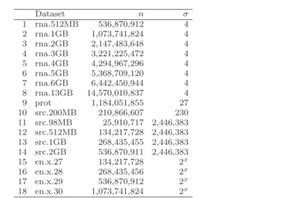
(14) 14. J. Fuentes-Sepúlveda, E. Elejalde, L. Ferres, D. Seco. 1 2 3 4 5 6 7 8 9 10 11 12 13 14 15 16 17 18. Dataset n σ rna.512MB 536,870,912 4 rna.1GB 1,073,741,824 4 rna.2GB 2,147,483,648 4 rna.3GB 3,221,225,472 4 rna.4GB 4,294,967,296 4 rna.5GB 5,368,709,120 4 rna.6GB 6,442,450,944 4 rna.13GB 14,570,010,837 4 prot 1,184,051,855 27 src.200MB 210,866,607 230 src.98MB 25,910,717 2,446,383 src.512MB 134,217,728 2,446,383 src.1GB 268,435,455 2,446,383 src.2GB 536,870,911 2,446,383 en.x.27 134,217,728 2x en.x.28 268,435,456 2x en.x.29 536,870,912 2x en.x.30 1,073,741,824 2x. Table 1: Datasets used in the experiments. In the datasets 15-18, x can take values in {4, 6, 8, 10, 12, 14}.. with 8 physical cores per NUMA node, clocking at 2.4GHz each, with one 64KB L1 instruction cache shared by two cores, one 16KB L1 data cache per core, a 2MB L2 cache shared between two cores, and a 6MB of L3 shared between 8 cores per NUMA node. The machine had 192GB of DDR3 RAM, clocking at 1333MHz, with 24GB per NUMA node. Algorithms were compared in terms of running times using the usual high-resolution (nanosecond) C functions in <time.h>. Memory usage was measured using the tools provided by malloc count [2]. The experimental trials consisted in running the algorithms on datasets of different alphabet sizes, input sizes n and number of cores. The datasets are shown in Table 1. We distinguish between two types of datasets: those in which symbols are encoded using 1 byte, and those in which symbols are encoded using 4 bytes. Datasets 1-10 in Table 1 with σ ≤ 256 were encoded using 1 byte. Datasets 11-14 were encoded using 4 bytes. Datasets 15-18, that have σ = 2x , were encoded as follows: for x = {4, 6, 8}, symbols were encoded with a single byte. For x = {10, 12, 14}, symbols were encoded in four bytes. The dataset rna.13GB is the GenBank mRNAs of the University of California, Santa Cruz4 . The rest of the rna datasets were generated by splitting the previous one. We also tested datasets of protein sequences, prot5 and source code, src.200MB6 . We also built a version of the source code dataset using words as symbols, src.98MB. The rest of the src datasets were generated by concatenating the previous one up to a maximum of 2GB. To measure the impact of varying the alphabet size, we took the English corpus of the Pizza & Chili website7 as a sequence of words and filtered the number of different symbols in the dataset. The dataset had an initial 4 http://hgdownload.cse.ucsc.edu/goldenPath/hg38/bigZips/xenoMrna.fa.gz (April, 2015) 5 http://pizzachili.dcc.uchile.cl/texts/protein/proteins.gz (April, 2015) 6 http://pizzachili.dcc.uchile.cl/texts/code/sources.gz (April, 2015) 7 http://pizzachili.dcc.uchile.cl/texts/nlang/english.1024MB.gz (March, 2013).

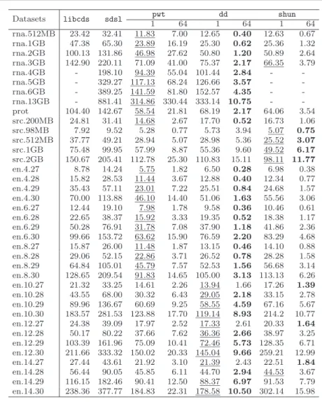
(15) Parallel Construction of Wavelet Trees on Multicore Architectures Datasets. libcds. sdsl. rna.512MB rna.1GB rna.2GB rna.3GB rna.4GB rna.5GB rna.6GB rna.13GB prot src.200MB src.98MB src.512MB src.1GB src.2GB en.4.27 en.4.28 en.4.29 en.4.30 en.6.27 en.6.28 en.6.29 en.6.30 en.8.27 en.8.28 en.8.29 en.8.30 en.10.27 en.10.28 en.10.29 en.10.30 en.12.27 en.12.28 en.12.29 en.12.30 en.14.27 en.14.28 en.14.29 en.14.30. 23.42 47.38 100.13 142.90 104.40 24.81 7.92 37.77 75.48 150.67 8.78 15.82 35.43 70.00 12.44 22.65 50.28 99.66 15.87 29.06 64.84 128.65 21.32 43.55 89.96 183.57 24.38 50.17 103.39 211.66 27.44 56.44 116.15 238.36. 32.41 65.30 131.86 220.11 198.10 329.27 389.25 881.41 142.67 31.41 9.52 49.21 99.95 205.41 14.24 28.53 57.11 113.88 19.10 38.37 76.91 153.72 26.00 52.15 105.01 209.54 33.25 68.00 136.67 281.53 39.09 80.22 161.96 333.32 43.61 90.05 182.46 377.77. pwt 1 64 11.83 7.00 23.89 16.19 46.98 27.62 71.09 41.00 94.39 55.04 117.13 68.24 141.59 81.80 314.86 330.44 58.54 21.81 14.68 2.67 5.28 0.77 28.94 5.07 57.99 8.87 112.78 25.30 5.75 1.82 11.44 3.67 23.01 7.22 46.10 14.40 7.98 1.78 15.92 3.33 31.78 7.08 63.62 15.90 11.48 1.87 22.86 3.71 45.79 7.57 91.83 14.65 14.61 2.26 30.32 6.43 60.69 9.25 123.88 17.70 17.97 2.52 37.66 7.62 75.09 10.41 150.02 20.33 21.92 3.10 45.85 6.11 90.41 12.50 184.83 22.31. dd 1 64 12.65 0.40 25.30 0.62 50.80 1.20 75.37 2.17 101.44 2.84 126.66 3.57 152.57 4.35 333.14 10.75 68.19 2.17 17.70 0.52 5.73 3.94 28.98 5.36 55.36 9.60 110.83 15.11 6.50 0.28 12.88 0.40 25.51 0.84 51.06 1.63 9.58 0.36 19.35 0.52 37.90 1.18 76.59 2.20 13.15 0.46 26.52 0.78 52.53 1.56 105.00 3.13 13.94 1.66 29.05 2.18 58.55 4.59 119.14 8.93 17.33 2.61 36.36 2.66 72.46 5.73 145.04 9.66 21.39 2.43 44.70 2.94 88.37 6.97 178.58 10.50. 15 shun 1 64 12.63 0.67 25.36 1.32 50.89 2.64 66.35 3.79 64.06 3.54 16.73 1.06 5.07 0.75 25.52 3.07 49.52 6.17 98.11 11.77 6.98 0.38 12.34 0.77 24.68 1.57 55.56 3.06 10.46 0.61 18.38 1.17 41.86 2.36 83.29 4.68 14.10 0.88 28.28 1.58 56.68 3.14 113.13 6.26 17.26 1.39 33.15 2.78 67.16 5.67 214.2 10.77 20.33 1.64 38.97 3.25 128.35 6.71 259.21 12.99 22.51 1.84 44.53 3.67 91.53 7.79 302.14 15.98. Table 2: Running times, in seconds, of the sequential algorithms and parallel algorithms with 1 and 64 threads. The best sequential times are underlined and the best parallel times are shown using bold typeface. A “-” is shown for implementations that just work for n < 232 .. alphabet Σ of σ=633,816 symbols. For experimentation, we generated an alphabet Σ ′ of size 2x , taking the top 2x most frequent words in the original Σ, and then assigning a random index to each symbol using a Marsenne Twister [23], with x ∈ {4, 6, 8, 10, 12, 14}. To create an input sequence S of n symbols for the English dataset (en), we searched for each symbol in Σ ′ in the original English text and, when found, appended it to S until it reached the maximum possible size given σ ′ (∼1.5GB, in the case of σ ′ = 218 ), maintaining the order of the original English text. We then either split S until we reached the target size n = 227 or concate-.

(16) 16. J. Fuentes-Sepúlveda, E. Elejalde, L. Ferres, D. Seco. nated S with initial sub-sequences of itself to reach the larger sizes 228 , 229 and 230 . We repeated each trial five times and recorded the median time [32]8 .. 4.2 Running times and speedup Table 2 shows the running times of all tested algorithms9. Libcds and shun work just for n < 232 , so we cannot report running times of these algorithms for the datasets rna.4GB, rna.5GB, rna.6GB and rna.13GB. For each dataset, we underline the best sequential running times. We use those values to compute speedups. The best parallel times for p = 64 are identified using a bold typeface. Although libcds and sdsl are the state-of-the-art in sequential implementations of wtrees, the best sequential running times were obtained from the parallel implementations running on one thread. The main reason for this is that Sdsl implements a semi-external algorithm for wtree construction, involving heavy disk access, while Libcds uses a recursive algorithm, with known memory and executions costs. Figure 5 shows speedups for rna.3GB, prot, src.200MB, en.4.30, src.2GB, en.14.30 datasets, with the largest n. As expected, the pwt algorithm is competitive until p < lg σ. Thus, for small σ the pwt algorithm is not the best alternative as shown in Figures 5a, 5b and 5d. If the algorithm recruits more threads than levels, the overhead of handling these threads increases, generating some “noise” in the times obtained. The performance of pwt will be dominated also by the thread that builds more levels. For instance, in Figure 5f we created a wtree with 14 levels. In the case of one thread, that thread has to build the 14 levels. In the case of 4 threads, each has to build three levels. For 8 and 12 threads, some threads will build two levels, so those threads dominate the running time. Finally, for the case of 16 threads, each thread has to build at most one level. This explains the “staircase” effect seen for pwt in Figure 5f. In all datasets shown in Figure 5, except for Figure 5e, the dd algorithm has a better speedup than both pwt and shun, especially for datasets with small alphabets, such as rna, prot and en.4. In the case of Figure 5e, shun has a better speedup, because our algorithms have worse data locality, we come back to the impact of locality of reference. It is important to remember that although shun has a better speedup, its memory consumption is larger than in our algorithms, as can be seen in Section 4.3.. 4.3 Memory consumption Figure 6 shows the amount of memory allocated with malloc and released with free. For all algorithms, we report the peak of memory allocation and only considered memory allocated during construction, not memory allocated to store the input text. The datasets are ordered incrementally by n. In the case of the dd 8 In order to be less sensitive to outliers, we use the median time instead of other statistics. In our experiments, the pwt algorithm showed a larger deviation with respect to the number of threads than the other algorithms. However the differences were not statistically significant. 9 A complete report of running times and everything needed to replicate these results is available at www.inf.udec.cl/~ josefuentes/wavelettree.

(17) 17. 32. Parallel Construction of Wavelet Trees on Multicore Architectures. ●. ●. ●. ●. ●. ●. ●. ● ●. ●. 14. 16. ● ●. Speedup. 18. 20. 24. 22. ●. ●. 12. Speedup. dd pwt shun. 26. 28. dd pwt shun. ●. ●. ●. ●. ●. ●. ●. ●. ●. ● ● ●. ●. 8 10. ● ●. 8. ●. ●. 4. 4. 6. 6. ●. ●. 2. 2. ●. ●. 0. 0. ●. 1. 8. 12. 20. 28. 36. 44. 52. 60. 1. 8. 12. 20. Number of threads. 26. dd pwt shun. 26. 36. 44. 52. 60. (b) prot, n ≈ 230 , σ=27. 30. (a) rna.3GB, n ≈ 232 , σ=4.. dd pwt shun. ●. ●. ●. ●. ●. ●. ●. ●. ●. 18 14. ●. Speedup. 14. Speedup. 18. 22. 22. ●. 28. Number of threads. ●. 8. ●. ●. ●. ●. ●. ●. ●. ●. ●. ● ●. 6. 6. ●. ●. 4. 4. ● ●. 2. 2. ●. ●. 0. 0. ●. 1. 8. 12. 20. 28. 36. 44. 52. 60. 1. 8. 12. 20. Number of threads. ●. ●. ●. ●. 52. 60. dd pwt shun. 16. ● ●. 14. ●. ●. ●. ●. ●. ●. ●. ●. ●. ● ●. ●. ● ● ●. 6. 4. ●. ●. 10. Speedup. 12. ●. 6. 44. (d) en.4.30, n = 230 , σ=16. ●. 8. 8. ●. ● ●. 36. 18. ●. ●. dd pwt ● shun. 28. Number of threads. (c) src.200MB, n ≈ 228 , σ=230.. Speedup. ●. ●. 8 10. 10. ● ●. ●. ●. ●. 2. 4. ●. ●. 2 ●. 0. ●. 1. 8. 12. 20. 28. 36. 44. 52. Number of threads. (e) src.2GB, n ≈ 229 , σ ≈ 221 .. 60. 1. 8. 12. 20. 28. 36. 44. 52. 60. Number of threads. (f) en.14.30, n = 230 , σ=214 .. Fig. 5: Speedup with respect to the best sequential time. The caption of each figure indicates the name of the dataset, the input size n and the alphabet size σ..

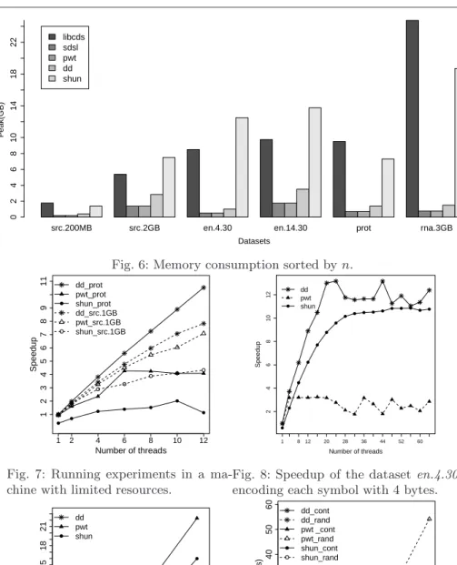
(18) 18. J. Fuentes-Sepúlveda, E. Elejalde, L. Ferres, D. Seco. algorithm, the figure shows memory consumption for k = 1. Libcds and shun use more memory during construction time. In fact, pwt uses up to 33 and 25 times less memory than Libcds and shun, respectively. Memory usage in libcds is dominated by its recursive nature, while shun copies the input sequence S, of O(n lg n) bits, to preserve it and to maintain permutations of it in each iteration. Additionally, shun uses an array of size O(σ lg n) bits to maintain some values associated to the nodes of the wtree, such as number of bits, the range of the alphabet, and the offset. In our algorithms and in sdsl, memory consumption is dominated by the arrays which store offset values, not by the input sequence. The main drawback of dd with respect to our own pwt is its memory consumption, since the latter increases with the alphabet size and the number of threads. For small alphabets, the working space of dd is almost constant. For instance, memory consumption for rna.2GB is 1GB, plus a small overhead for each new thread. For larger alphabets, such as src.2GB with σ ≈ 222 , the working space increases linearly with the number of threads, using 1.46GB with 1 thread and 2.5GB with 12 threads. Fortunately, most of the sequences used in real-world applications have an alphabet size smaller than 217 . Such is the case of DNA sequences, the human genome, natural language alphabets (Unicode standard), etc.10.. 4.4 Other experiments In order to have a better understanding of our algorithms, we performed the following experiments: Limited resources. When memory is limited, algorithms such as Libcds and shun suffer a decrement in their performance. This is evident in Figure 7, where we tested the parallel algorithms with datasets prot and src.1GB11 on a 12-core computer with 6GB of DDR3 RAM12 . In this new set of experiments, the speedup of our algorithms exceeded the speedup shown by shun, both for datasets where we previously showed the better performance (see Figure 5b) and for datasets where previously shun showed better performance (see Figure 5e and Table 2). Encoding. We observed that the encoding of the symbols of the original sequence has a great impact in the speedups of the construction algorithms. Figures 5a–5d have speedups greater than 27x, while there is a noticeable performance degradation in Figure 5e and Figure 5f. This is due to an encoding subtlety: The datasets used in the experiments resulting in Figures 5a–5d are encoded using one byte, while the other used four bytes. To prove the impact of the encoding in the performance of the construction algorithms, we repeated the experiments using a dataset that used four bytes per symbol for σ ≤ 28 . Figures 5d and 8 show the influence of 10. The Unicode Consortium: http://www.unicode.org/ The construction times of shun with the src.2GB dataset exceeds one hour. To make the algorithms in the figures comparable, we report the running times for the dataset src.1GB. 12 The computer tested is a dual-processor Intel R Xeon R CPU (E5645) with six cores per processor, for a total of 12 physical cores running at 2.50GHz. Hyperthreading was disabled. The computer runs Linux 3.5.0-17-generic, in 64-bit mode. This machine has per-core L1 and L2 caches of sizes 32KB and 256KB respectively and 1 per-processor shared L3 cache of 12MB, with a 5,958MB (∼6GB) DDR3 RAM. 11.

(19) Parallel Construction of Wavelet Trees on Multicore Architectures. 2. 4. 6. 8. 10. 14. 18. 22. libcds sdsl pwt dd shun. 0. src.200MB. src.2GB. en.4.30. en.14.30. prot. rna.3GB. Datasets. dd pwt shun. ●. 10. ●. ●. ●. ●. ●. ●. ●. ●. ●. ●. ●. 8. ● ●. ●. 6. Speedup. ●. 12. dd_prot pwt_prot shun_prot dd_src.1GB pwt_src.1GB shun_src.1GB. 4. ●. ● ●. ●. ●. 4. 6. 8. ●. ●. 2. Speedup 1 2 3 4 5 6 7 8 9. 11. Fig. 6: Memory consumption sorted by n.. ● ● ●. 1. 2. 10. 12. 1. 8. 12. 20. Number of threads. 28. 36. 44. 52. 60. Number of threads. 50. 18. ●. dd pwt shun ●. ●. dd_cont dd_rand pwt _cont pwt_rand shun_cont shun_rand. ●. ●. ●. 210. 212. ●. ●. ●. 10. ●. Time(secs) 20 30 40. 21. 60. Fig. 7: Running experiments in a ma-Fig. 8: Speedup of the dataset en.4.30 chine with limited resources. encoding each symbol with 4 bytes.. ● ●. 0. Time(secs) 1 3 5 7 9 12 15. Peak(GB). 19. 227. 228. 229. Size of sequence (n). 230. 24. 26. 28. Size of alphabet ( σ ). 214. Fig. 10: Time over σ for the best and Fig. 9: Time over n with σ = 214 , 64 average cases with n = 230 and p = lg σ threads and en.14 datasets. threads..

(20) 20. J. Fuentes-Sepúlveda, E. Elejalde, L. Ferres, D. Seco. encoding. As expected, the greater the memory used for encoding, the worse the perfomance. On multicore architectures, some levels of the memory hierarchy are shared by different cores. This increases the rate of memory evictions. Hence, it is crucial to reduce the number of memory transfers. Besides, in NUMA architectures, where each NUMA node has a local RAM and the transfers between local RAMs is expensive, the reduction of memory transfers is critical. In the case of one byte per symbol, each memory transfer carries four times more symbols than in the case of four bytes per symbol, effectively helping reduce memory transfers. Influence of the size of sequence. Figure 9 shows that for the en.14 dataset, fixing the number of threads to 64 and σ to 214 , for larger n the domain decomposition algorithm behaves better in running time than the pwt algorithm and Shun’s algorithm. In other words, with more cores and enough work for each parallel task, the dd algorithm should scale appropriately. Influence of the locality of reference. Theoretically, fixing n and varying σ with p = lg σ threads, the pwt algorithm should show a constant-time behavior, no matter the value of σ. However, in practice, the running times of pwt increase with the alphabet size. The reason for this difference in theoretical and practical results is that levels closer to the leaves in the wtree exhibit a weaker locality of reference. In other words, locality of reference of the pwt algorithm is inversely proportional to σ. Additionally, the dynamic multithreading model assumes that the cost of access to any position in the memory is constant, but that assumption is not true in a NUMA architecture. In order to visualize the impact of the locality of reference over running times, we generate two artificial datasets with n = 230 , Σ = {1 . . . 2y }, with y ∈ {4, 6, 8, 10, 12, 14} and encoding each symbol with four bytes. The first dataset, cont, was created writing n/σ times each symbol of Σ and then sorting the symbols according to their position in the alphabet. The second dataset, rand, was created in a similar fashion, but writing symbols at random positions. The objective of the cont dataset is to force the best case of the pwt algorithm, where the locality of reference is higher. In contrast, the rand dataset forces the average case, with a low locality of reference. In these experiments, we used the optimal number of threads of pwt, that is, p = lg σ. Besides, we allocated evenly the memory over the NUMA nodes to ensure constant access cost to any position in the memory13. The results are shown in Figure 10. In its average case, dashed lines, the performance of the pwt algorithm is degraded for larger alphabets because locality of reference is low, increasing the amount of cache misses, and thus degrading the overall performance. In the best case, solid lines, the pwt shows a practical behavior similar to the theoretical one. Since the dd algorithm implements the pwt algorithm to build each partial wtree, the locality of reference impacts also on its performance. However, because the construction of the partial wtrees involves sequences of size O(n/p), the impact is less than in the pwt algorithm. Finally, Shun’s algorithm is insensitive to the distribution of the symbols in the sequence. The study of the impact of the architecture on the construction of wtrees and other succinct data structures, and the improvement of the locality of reference of our algorithms are interesting lines for future research. 13 To ensure the constant access cost, we use the numactl command with “interleave=all” option. The command allocates the memory using round robin on the NUMA nodes..

(21) Parallel Construction of Wavelet Trees on Multicore Architectures. 21. 4.5 Discussion. In most cases, the domain decomposition algorithm, dd, showed the best speedup. Additionally, dd can be adjusted either in favor of running time or memory consumption. pwt showed good scalability, but up to p < lg σ. This limitation may be overcome by using pwt as part of dd, dividing the input sequence in an adequate number of subsequences. With respect to working space, pwt was the algorithm with lowest memory consumption. This is important because an algorithm with low memory consumption can be executed in machines with limited resources, can reduce cache misses due to invalidations (false sharing) and can therefore reduce energy consumption. Even though memory consumption of the dd algorithm increases with the number of subsequences, it can be controlled manipulating the number of segments. In the case of shun, its memory consumption is too large to be competitive in machines with limited memory. The encoding and the distribution of the symbols of the input sequence impact the performance of the algorithms. All the parallel algorithms introduced here show a better speedup for encodings that use less bits because there are less memory transfers. Our algorithms are also sensitive to the distribution of the symbols. When the symbols are randomly distributed, the locality of reference is worse in comparison with more uniform distributions. This gives us a hint to improve the performance of our algorithms in the future. To sum up, in general, the dd algorithm is the best alternative for the construction of wtrees on multicore architectures, considering both running time and memory consumption. For domains with limited resources, pwt, which is a building block of dd, arises as a good alternative on its own.. 5 Conclusions and future work Despite the vast amount of research on wavelet trees, very little has been done to optimize them for current ubiquitous multicore architectures. We have shown that it is possible to have practical multicore implementations of wavelet tree construction by exploiting information related to the levels of the wtree, achieving O(lg n)-time construction and good use of memory resources. In this paper we introduced two multicore algorithms for parallel construction of wtrees. Our domain decomposition algorithm, dd, may be used in any domain, but in those contexts where it is not possible to use all available resources, our perlevel algorithm, pwt, may be more suitable. We have focused on the most general representation of a wtree, but some of our results may apply to other variants. For example, it would be interesting to study how to extend our results to compressed wavelet trees (e.g., Huffman shaped wtrees) and to generalized wavelet trees (i.e., multiary wavelet trees where the fan out of each node is increased from 2 to O(polylog(n))). Also, it is interesting to explore the extension of our results to the Wavelet Matrix [8] (a different level-wise approach to avoid the O(σ lg n) space overhead for the structure of the tree, which turns out to be simpler and faster than the wavelet tree without pointers). Future work also involves dynamization, whereby the wtree is being modified concurrently by many processes as it is queried, though dynamic succinct data structures, even sequential ones is still an open area.

(22) 22. J. Fuentes-Sepúlveda, E. Elejalde, L. Ferres, D. Seco. of research. A further line of work involves the design of cache-aware algorithms to construct wtrees, obtaining more efficient implementations, both in time and in memory resources. In our previous work [15] we studied the parallelization of some queries on wtrees. The parallelization of other queries is yet another interesting future work. For all our construction algorithms we assume that the input sequence S fits in memory. However, we can extend our results to the construction of wtrees where the input sequence S and the wtree do not fit. Following some implementation ideas of Sdsl[16], we can read the input sequence in buffers to construct partial wtrees for each buffer and finally merge all of them to obtain the final wtree. In more detail, we can extend our algorithms as follows: 1. Read the input sequence S using a buffer of size b. We can use the portion of main memory that will not be used by the wtree as the buffer. 2. Create a partial wtree without rank/select structures taking the buffer as input. The partial wtree can be constructed in parallel using our dd algorithm with O(b lg σ/p) time and O(1) span. (We could also use the pwt if the available memory is scarce). The starting position of each node in the partial wtree is stored in a bidimensional array L. 3. Repeat steps 1 and 2 until the complete input sequence is read. 4. After the complete input sequence is read, we compute the final position of the nodes of all the partial wtrees. These positions are computed performing a parallel prefix sum[19] over the values of the arrays L’s, similar to the dd algorithm. It takes O(bσ/p + lg p) time and O(lg(bσ)) span. 5. The final wtree is constructed using Function mergeBA with O(n lg σ/pw) and O(1) span, where w is the word size of the architecture. The extension takes O(n lg σ/p + bσ/p + lg p) time and O(n/b + lg(bσ)) span. Notice that this idea is similar to the dd algorithm and it can be applied on multiple levels. For example, it can be used on distributed architectures, where the buffers are processed by different machines, and one machine merges all the partial wtrees. Additionally, observe that we can use the entire main memory as the buffer, storing the partial wtrees and the L arrays on disk each time we finish the processing of a buffer. We leave the implementation and empirical evaluation of these ideas as future work. It has become evident that architecture has become relevant again. It is nowadays difficult to find single-core computers. Therefore, it seems like a waste of resources to stick to sequential algorithms. We believe one natural way to improve performance of important data structures, such as wavelet trees, is to squeeze every drop of parallelism of modern multicore machines.. References 1. Arroyuelo, D., Costa, V.G., González, S., Marı́n, M., Oyarzún, M.: Distributed search based on self-indexed compressed text. Inf. Process. Manag. 48(5), 819–827 (2012). DOI http://dx.doi.org/10.1016/j.ipm.2011.01.008 2. Bingmann, T.: malloc count - tools for runtime memory usage analysis and profiling. http://panthema.net/2013/malloc_count/ (2013). Last accessed: January 17, 2015 3. Blumofe, R.D., Leiserson, C.E.: Scheduling multithreaded computations by work stealing. J. ACM 46(5), 720–748 (1999). DOI 10.1145/324133.324234.

(23) Parallel Construction of Wavelet Trees on Multicore Architectures. 23. 4. Brisaboa, N.R., Luaces, M.R., Navarro, G., Seco, D.: Space-efficient representations of rectangle datasets supporting orthogonal range querying. Inf. Syst. 38(5), 635–655 (2013). DOI 10.1016/j.is.2013.01.005 5. Burrows, M., Wheeler, D.J.: A block-sorting lossless data compression algorithm. Tech. rep., Digital Equipment Corporation (1994) 6. Claude, F.: A compressed data structure library. https://github.com/fclaude/libcds (2011). Last accessed: August 13, 2015 7. Claude, F., Navarro, G.: Practical rank/select queries over arbitrary sequences. In: SPIRE, pp. 176–187. Springer, Berlin, Heidelberg (2009). DOI 10.1007/978-3-540-89097-3 18 8. Claude, F., Navarro, G.: The wavelet matrix. In: SPIRE, vol. 7608, pp. 167–179. Springer, Berlin, Heidelberg (2012). DOI 10.1007/978-3-642-34109-0 18 9. Claude, F., Nicholson, P.K., Seco, D.: Space efficient wavelet tree construction. In: SPIRE, vol. 7024, pp. 185–196. Springer, Berlin, Heidelberg (2011) 10. Cormen, T.H., Leiserson, C.E., Rivest, R.L., Stein, C.: Introduction to Algorithms, third edn., chap. Multithreaded Algorithms, pp. 772–812. The MIT Press (2009) 11. Faro, S., Külekci, M.O.: Fast multiple string matching using streaming SIMD extensions technology. In: SPIRE, pp. 217–228. Springer, Berlin, Heidelberg (2012). DOI 10.1007/ 978-3-642-34109-0 23 12. Ferragina, P., Manzini, G.: Opportunistic data structures with applications. In: Proceedings of the 41st Annual Symposium on Foundations of Computer Science, FOCS ’00, pp. 390–. IEEE Computer Society, Washington, DC, USA (2000). URL http://dl.acm.org/citation.cfm?id=795666.796543 13. Ferragina, P., Manzini, G., Mäkinen, V., Navarro, G.: String Processing and Information Retrieval: 11th International Conference, SPIRE 2004, Padova, Italy, October 58, 2004. Proceedings, chap. An Alphabet-Friendly FM-Index, pp. 150–160. Springer Berlin Heidelberg, Berlin, Heidelberg (2004). DOI 10.1007/978-3-540-30213-1 23. URL http://dx.doi.org/10.1007/978-3-540-30213-1_23 14. Ferragina, P., Manzini, G., Mäkinen, V., Navarro, G.: Compressed representations of sequences and full-text indexes. ACM Trans. Algorithms 3(2) (2007). DOI 10.1145/1240233. 1240243 15. Fuentes-Sepúlveda, J., Elejalde, E., Ferres, L., Seco, D.: Efficient Wavelet Tree Construction and Querying for Multicore Architectures. In: J. Gudmundsson, J. Katajainen (eds.) Experimental Algorithms, Lecture Notes in Computer Science, vol. 8504, pp. 150–161. Springer International Publishing (2014). DOI 10.1007/978-3-319-07959-2\ 13. URL http://dx.doi.org/10.1007/978-3-319-07959-2_13 16. Gog, S.: Succinct data structure library 2.0. https://github.com/simongog/sdsl-lite (2012). Last accessed: January 17, 2015 17. González, R., Grabowski, S., Mäkinen, V., Navarro, G.: Practical implementation of rank and select queries. In: WEA, pp. 27–38. CTI Press, Greece (2005). Poster 18. Grossi, R., Gupta, A., Vitter, J.S.: High-order entropy-compressed text indexes. In: SODA, pp. 841–850. Soc. Ind. Appl. Math., Philadelphia, PA, USA (2003) 19. Helman, D.R., JáJá, J.: Prefix computations on symmetric multiprocessors. J. Par. Dist. Comput. 61(2), 265 – 278 (2001). DOI http://dx.doi.org/10.1006/jpdc.2000.1678 20. Illumina, Inc.: An Introduction to Next-Generation Sequencing Technology (2016). URL http://www.illumina.com/content/dam/illumina-marketing/documents/products/illumina_sequencing_introduction.pdf 21. Ladra, S., Pedreira, O., Duato, J., Brisaboa, N.R.: Exploiting SIMD Instructions in Current Processors to Improve Classical String Algorithms. In: ADBIS, pp. 254–267. Springer, Berlin, Heidelberg (2012). DOI 10.1007/978-3-642-33074-2 19 22. Makris, C.: Wavelet trees: A survey. Comput. Sci. Inf. Syst. 9(2), 585–625 (2012) 23. Matsumoto, M., Nishimura, T.: Mersenne twister: a 623-dimensionally equidistributed uniform pseudo-random number generator. ACM Trans. Model. Comput. Simul. 8(1), 3–30 (1998). DOI 10.1145/272991.272995 24. Navarro, G.: Wavelet trees for all. In: CPM, pp. 2–26. Springer, Berlin, Heidelberg (2012). DOI 10.1007/978-3-642-31265-6 2 25. Navarro, G., Nekrich, Y., Russo, L.M.S.: Space-efficient data-analysis queries on grids. Theoret. Comput. Sci. 482, 60–72 (2013). DOI 10.1016/j.tcs.2012.11.031 26. Pantaleoni, J., Subtil, N.: Nvbio library. URL http://nvlabs.github.io/nvbio/index.html . Accessed April 12th, 2016 27. Raman, R., Raman, V., Satti, S.R.: Succinct indexable dictionaries with applications to encoding k-ary trees, prefix sums and multisets. ACM Trans. Algorithms 3(4) (2007). DOI 10.1145/1290672.1290680.

(24) 24. J. Fuentes-Sepúlveda, E. Elejalde, L. Ferres, D. Seco. 28. Schnattinger, T., Ohlebusch, E., Gog, S.: Bidirectional search in a string with wavelet trees and bidirectional matching statistics. Information and Computation 213, 13 – 22 (2012). DOI http://dx.doi.org/10.1016/j.ic.2011.03.007. URL http://www.sciencedirect.com/science/article/pii/S0890540112000235 . Special Issue: Combinatorial Pattern Matching (CPM 2010) 29. Shun, J.: Parallel wavelet tree construction. In: Proceedings of the IEEE Data Compression Conference, pp. 63–72. Utah, USA (2015). DOI 10.1109/DCC.2015.7 30. Singer, J.: A wavelet tree based fm-index for biological sequences in seqan. Master’s thesis, Freie Universität Berlin (2012). URL http://www.mi.fu-berlin.de/wiki/pub/ABI/FMIndexThesis/FMIndex.pdf 31. Tischler, G.: On wavelet tree construction. In: CPM, pp. 208–218. Springer, Berlin, Heidelberg (2011) 32. Touati, S.A.A., Worms, J., Briais, S.: The Speedup-Test: A Statistical Methodology for Program Speedup Analysis and Computation. Concurrency and Computation: Practice and Experience 25(10), 1410–1426 (2013). DOI 10.1002/cpe.2939. URL https://hal.inria.fr/hal-00764454. Article first published online: 15 OCT 2012 33. Välimäki, N., Mäkinen, V.: Space-efficient algorithms for document retrieval. In: CPM, LNCS, vol. 4580, pp. 205–215. Springer, Berlin, Heidelberg (2007). DOI 10.1007/ 978-3-540-73437-6 22 34. Wetterstrand, K.A.: Dna sequencing costs: Data from the nhgri genome sequencing program (gsp). URL http://www.genome.gov/sequencingcosts. Accessed April 12th, 2016.

(25)