Al based robust multi regime controller

Texto completo

(1)TECNOLÓGICO DE MONTERREY. EMbUoteca. ~Ciudad~~. Instituto Tecnológico y de Estudios Superiores de Monterrey. Escuela de Ingeniería. v Ciencias. Campus Ciudad de México. Al-based robust multi-regime controller Tesis que presenta: Luis Miguel lbarra Moyers. Para obtener el grado de: Doctor en Ciencias de Ingeniería. Asesor de tesis: Dr. Pedro Ponce Cruz Ca-Asesor: Dr. Arturo Molina Gutiérrez México, D.F., abril 2016.

(2) Contents 1. Introduction 1.1 Uncertainty decoupling . . . . . . . . . . . . . . 1.2 Accomplishment as a means to decision making. 4. 4. 7. 2. Control theoretical basis 11 2.1 Cascade control . . . . . . . . . . . . . . . . . . . . . . . . . . . . . . . . . . . . 11 2.2 Quantitative feedback theory 12 2.3 Direct Torque Control (DTC) . . . . . . . . 15 2.3.1 VSI inverter and d-q transformation 15 2.3.2 Modulation techniques . 17 20 2.3.3 Traditional DTC 2.3.4 SVPWM-DTC 25. 3. Robust control of a voltage buck converter through traditional 3.1 Small-signal state-space averaging 3.2 PID tuning through LQR approach . . . . . . . . . . . . . . . . . . 3.2.1 Specific design for Buck converter 3.2.2 QFT design for buck converter . . . . . . . . . . . . . . . . 3.3 Incorporation of voltage through cascade QFT dcsign 3.3.1 Specific design for buck converter . . . . . . . . . . . . . . . 3.4 Simulation results 3.5 Discussion . . . . . . . . . . . . . . . . . .. QFT. 27 29 . . . . . . . . . . 31 33 . . . . . . . . . . 34 39 . . . . . . . . . . 40 43. ........... 46. 4. Robust control of an induction motor through traditional QFT 49 4.1 QFT settings obtainment . . . . . . . . . . . . . . . . . . . . . . . . . . . . . . . . . 50 4.2 Controller adjustment and pre-filter 52 4.3 Simulation Results 53 4.4 Discussion . . . . . . . . . . . . . . . 54. 5. Accomplishment membership functions 5.1 Uncertainty basis . . . . . . . . . . . 5.2 Uncertain boundaries . . . . . . . . . 5.3 A new approach to subnormal MFs . 5.4 Description of DA-MFs . . . . . . . 5.5 Ellipsoidal rules and their fuzzy interpretation .. ¡¡. 56 56 58 59. 62 68.

(3) CONTENTS. m. 6 Uncertainty decoupling and robust control 6.1 Dealing with cascaded uncertainty 6.1.1 Plant homogenization . . . 6.1.2 Pre-filtering . . . . . . . . . 6.1.3 Controller effort reduction . 6.1.4 Cascaded topology 6.2 Standard examples 6.2.1 Example 1 . . . . . 6.2.2 Example 2. . . . . 6.3 Uncertainty decoupled robust control of a voltage buck converter. 71 71 73 74 76 81 84 84 88 92. 7 Gain scheduling for multi-regime robust control of an induction motor 7.1 Controller characteristics . . . . . . . . 7.2 Design process for an induction motor 7.2.1 Robust control design 7.2.2 Gain scheduling. 7.3 Results . . . 7.4 Discussion .. 97 99 101 102 105 107 108. 8 Conclusions. 109.

(4) Abstract Uncertainty in nature makes impossible to derive a simple controller which satisfactorily amends a given plant's variations. Additional considerations must be made in order to design a compensator which tackles the variability; this has been traditionally performed through two different approaches: robust and adaptive control. The former will "absorb" the variability so its design commonly results in a complex structure and overall high ga,in. The later uses additional measurements or calculations to modify a base controller depending on plant's changes. As the control problem becomes more demanding and specific, aforementioned approaches fail to deliver a simple yet effective controller. For those cases where a clear separation can be made over control objectives in terms of expected performance, the combination of both techniques can improve not only system's close-loop behavior but the controller's effort, for EXample. This collaborative perspective would also help define which part of the uncertainties are addressed by which methodology and clearly separate design objectives regarding fault states or nonlinearities. The present proposal's objectives are twofold.. On th,~ one hand, a way to derive a robust. controller which accounts for uncertainty decoupling and controller's effort awareness is presented. On the second hand, a fuzzy scheduling scheme (using accc)mplishment membership functions) is added to that cascaded robust topology to achieve multi-regime control. The first objective is validated towards two standard examples and a case study involving a voltage converter. Similarly, the second approach is tested over the startup of a simulated induction motor with parametric variations and unknown required mechanical torque. This last example combines both perspectives in order to amend parametric variations through robust control, and different operating regimes by fuzzy blending. This makes the design process clearer and '.mproves system's output performance. A set of robust controllers are designed to <leal with the parametric variations at each regime,. while the load changes are to be faced by a fuzzy inference engine. As the robust controllers are forced to have the same structure, they can be seen as a single controller whose parameters. 1.

(5) CONTENTS. 2. vary depending on the fuzzy decision making. In addition, their individual design process is done on the frequency-domain so the complete tuning process is simple, quantifiable, and controller's effort-aware. The uncertainty decoupling for cascaded control topologies, as the main contribution of this work, is tested against similar proposals and its merits are clearly shown. Due to the deep inspiration found on Quantitative Feedback Theory (QFT), much effort is made to exhibit the main differences between the present proposal and the traditiona:. design perspective of QFT control design. Furthermore, the problem is extended to a multi-regirne system subjected to fuzzy blending, where accomplishrnent membership functions (another coll":ribution) are used to build its fuzzyfication phase. The system to be tested is an induction motor with parametric and output torque variations, where the parameter's uncertainty can account for time dependency and faulty states, and the torque variations respond to different operating regimes (whose transit may be nonlinear). Motor's torque and speed are first decoupled through Dire-=t Torque Control (DTC) technique so simple Voltage Source Inverter (VSI) can be used to regulate torque through voltage vector commands without extra position sensors. A traditional QFT robust controller is designed parallel to validate the present proposal in terms of controller?s complexity, design objectives, and close-loop results. This document presents, in an ordered fashion, the r2search efforts devoted to uncertainty description and its management in dynamic systems. As s-1ch, it includes the contents of various rcsearch papers, product of systematic proposals towards intelligent and robust control, as well as unpublished case studies which assemble them. Part of the information and findings exhibited in this document are also available in published works [91, 44, 46, 45, 47]; the perspective taken in this work is that of presenting those contributions as systernatic steps in pursuit of an uncertaintydecoupling multi-regime controller. The structure of this document is as follows. Firstly, an introduction to uncertainty is provided on Chapter 1 from both, the dynamic system's point of view, related to robust control, and the fuzzy interpretation subjected to variability. Secondly, the theoretical foundations pertaining cascade and robust control, QFT, and electric motors' commutation techniques and control are provided in Chapter 2. Chapters 3 anc:i 4 show the application of the QFT traditional methodology to a voltage buck converter andan induction motor (respectively), in order to validate its usage and set a framework to enlighten the novelty of the actual proposaJ of this work. The fuzzy perspective is resumed in Chapter 5 where the accomplishment membership functions are fully explained so.

(6) CONTENTS. 3. its further usage is conceptually consistent. Lastly, Chapt2r 6 presents the main contribution of this document by explaining the uncertainty-decoupling mEthodology and applying it to the same voltage converter previously addressed, and Chapter 7 exter.ds the example of Chapter 4 by adding multi-regime capabilities to a control topology by including uncertainty decoupling concepts and a fuzzy scheduling system based on accomplishment membernhip functions..

(7) Chapter 1. Introduction 1.1. U ncertainty decoupling. l\fathematical models can be used to approximate the physkal reality of an event. They are indeed called approximations due to the mismatch found if compared towards the plant they model. There are severa! sources of such variability as: Unknown characteristics, uncertain conditions. overall disturbances, and noisy /biased measurements [118]. However, if the model is considered to actually represent a given plant, there are sorne remaining considerations regarding how effectively system's variations or natural complexity is to be amended. Most models misses sorne physical characteristics due to mathematical limitations or required simplifications. Moreover, plant's time-variations, disturbances, and modes of operation impose new restrictions to them, confining their usefulness to specific situations. Consequently, the complexity lost while mocleling should be compensated by the control.er, which must be dependable enough to provide a good performance in spite of uncertainties ancl variations. Such a controller is called to be robust as it can control a group of systems [51] within a safe area of operation. Indeed, that area tries to endose aforementioned variability by considering marginal worst-case models. This approach has solved complex modeling problems like in [118] where an airplane surface subjected to fault is analyzed. Dueto its nature, a robust controller is conservative, complex, and non-optima!. This is bearable as it furnishes a way to control time-variant, nonlinear, and uncertain plants in relatively simple ways.. However, robustness and performance specificatious will increase required control effort. [73, 15], hindering actual realization. Moreover, setting limits to controller effort is complicated [108] and establishes a trade-off compromising desired beha.vior. Therefore, new design techniques 4.

(8) CHAPTER l. INTRODUCTION. 5. are needed to relax, simplify, and bound the controller effort while preserving sorne of the desired performance as said in [63]. Many works have focused on H00 methods whose result is a controller which satisfies an infinitynorm bounded operating area. H 00 controllers have large gains which derive in large control effort. As a consequence, suboptimal controllers are preferred due to easier realization [97]. In arder to avoid controller's complexity, other methods have been proposed as in [51] where the infinity norm is fulfilled by PID controllers, tuned by evolutionary algorithms. In [41] the robustness is achieved by a fuzzy Sugeno controller, which explicitly takes into account control effort. Regardless the specific methodology to be followed, most works assume sorne knowledge about the boundaries where the uncertainties reside. More recently, works on nonlinear systems have been published where this restriction is fulfilled [43, 9]. Other proposals likE Quantitative Feedback Theory (QFT) and cascade dependent topologies are covered later in this work to emphasize their merits and frame the present propasa!. Although robust control operates over a "safe" area, it <loes not imply that plant knowledge can be poor o:- limited. The most a designer knows about a plant, the less critica! performance trade-offs will be. Actuators saturation [73], plant's total bandwidth [15], and inherent instability [52] (among many others) directly affect regulation and tracking conditions. Plant knowledge can be improved, far instance, by adding extra measurements or integrating observers. Many works have focused cm expanding the robustness/performance capabilities of a system like [103] where a robustness measurement is associated to the relation between the inner and outer loops of a cascaded structure. A different perspective which compensate variability on a DC /DC con verter by using observers is shown in [56]. Whether a robust controller is designed under ignorance of plant details, its scope will be restricted. Whenever modeling can not cope with precision and simplicity, different alternatives are needed. In an effort to generalize common processes, an approximation to fixed-order cascaded loops is used in [111]. In this case, the real dynamics are absorbed by "sufficient" transfer functions, taking advantage of secondary measurements. A similar ca.se can be found in [50] where B-Splines are used to capture the system response and then, to tune both of the cascaded controllers. Various techniques (sorne mentioned above) focus on PID controllers dueto their industrial availability and relative simplicity, avoiding more "complex" control topologies. However, controller complexity is not unjustified when dealing with equally complex plants and high performance specifications. In this spirit, the present propasa! aims to make controller complexity designer-dependent, while.

(9) 6. CHAPTER l. INTRODUCTION. providing a simple methodology to associate cascaded dynamics (unrelated to identification or regression) ancl constraining controller effort (with no use of optimization processes). As introduced above, control effort is an important restriction when dealing with physical system's constraints. This characteristic should be observecl as the energy used to manipulate the plant is limited, and the related actuators have input limit specifications as well as a restricted output, so saturation can occur [108]. Optima! control is commonly achieved by including a cost function regarding controller effort on the design process. Equivalent and novel approaches to this methodology have been proposed as in [113] where "feedback eigenvector assignment" is used, or [24] where the problem is solved by manipulating the input reference value to obtain a safe controller output. Manipulating the admitted controller's output will obviously affect response speed as stated by [60, 24], where the aforementioned trade-off is related to plant's bandwidth. Consequently, sorne technique is needed to permit fast and optima! operation to sorne extent. The improvement of these two variables together is contradictory; however, it should be possible to add design freedorn so their importance is weighted as desired. As stated in [108], the maximum usage of actuator capabilities is sornetimes wanted, even if its operation implies a bang-bang controller output. The method presented in this document allows the viwalization and management of the effort /speed trade-off. It is noteworthy that this capability is implemented through bounded operating conditions as most optima! or robust techniques. Bounded error signals entail a new restriction (must be predefined) which, in turn, allow controller rea!ization.. In the same manner, robust. control considers an operating area defined by error interYals which must be taken into account by the controller. Again, if the controller is designed to face the worst-case scenario, it will be conservative but dependable. Boundedness allows, for instance, the explicit computation of a given controller like in [73]. It also permits the fulfilling of a certain norm for any of the aforementioned requirements; specifically, the design of a fuzzy controller which observes this kind of dependency is shown in [41]. It is the interest of this work to present a single robm,t controller conformed by all the subcontrollers as collaborative entities. In this way, bandwidth separation is desired but not enforced, and tuning is presented as a step-by-step process related to subprocess hierarchy. The cascaded topology could be extended ton subprocesses whether it is physically realizable, preserving robustness, control effort awareness, disturbance rejection, and easy tuning. A similar approach can be found in [120] and [119] which, however, does not observe control effort reduction and propases.

(10) 7. CHAPTER l. INTRODUCTION. a very conservative way to embed the loops' characteristics as moving outwards in the cascaded topology. The way robustness is achieved in this work is based on QFT methodology: however, it avoids the usage of time-domain restriction bands and propases a different way to take advantage of the pre-filter to reduce controller's effort.. 1.2. Accomplishment as a means to decision making. The traditional set theory considers a set to be a grouping of objects S. = {s }. Those elements are. known to belong to the set by the intuition of containment; however, if the set has a subscribed label, i.e. it represents a concept, the membership of each element to the set can be partial. This was proposed by Zadeh [125], generalizing set theory so the elements of a set belong to it to a certain extent, depending on how related they are to thE concept in question.. A membership. function (MF) µA (s) : s E R --t [O, 1], assigns a 1 to an element which is completely represented by. A's label, while a O implies that the element can not be co::isidered as a part of A. So a fuzzy set can be represented as a pair A= {s,µA(s)}; A~ S. Dubois and Prade offered three different ways to understand l'v1Fs as pointed by Medasani et al. [82]: If µA(x) = 0.8, (a) 80% of the population declared that x belongs to A (likelihood), (h) 80% of the population described A asan interval which contained x (random set view), and (c) x is at a normalized dista.nce equal to 0.2 from the ideal prototype of A (typicality). Independent to the interpretation of the ::'vIF, it is clear that 1:he result of the proposition "x is A'' can not be true or false, but uncertain. Several techniques to <leal with uncertainty through MFs have been developed. An early survey by Medasani et al. [82] reveals that there is not a specific way to face uncertainty representation and that MFs can be variously defined. They also categorize these approaches depending on their underlying pri::iciple as: polling, typicality, heuristic, probability-related, histogram frequency analysis, artificial neural networks, clustering, and mixture decomposition. Fuzzy logic has provided a way to express uncertainty by capturing the vagueness of linguistic, qualitative, incomplete, or noisy information. Traditionally, uncertainty has been addressed by probability theory as imprecision in variable representation is considered to be statistical in nature. However, the linguistic approximation made by Zadeh allows this vagueness to be addressed in the spirit of its meaning [126]. By adding this distinction, Zad,~h attached a possibility interpretation to membership degrees. Although, as said before, there is no specific way to interpret MFs, they.

(11) CHAPTER l. INTRODUCTION. 8. are commonly considered as possibility distributions. Possibility theory has been comprehensively surveyed by Dubois [29]. In the eyes of this author, possibility can be objective when it models a physical property in nature, or epistemic if the uncertainty is derived from the state of knowledge of an agrnt. There are four ways to understand possibility: Feasibility (ease of achievement), plausibility (propensity), in a logical manner (it is compliant to sorne information), and deontic (permitted by the law). From these perspectives, the plausibility is the most commonly adopted in research works as it directly shows how sure we are about a certain proposition. Plausibility is also dual rela1;ed to certainty as the later reflects a lack of plausibility of an opposite proposition. However, possibility distributions are not the only mechanism to address incompleteness and parallel conceptual-mathematical approaches have been designed and tested. Uncertainty has been faced through different concepts: capacity, belief, plausibility, possibility, and necessity among others. Besides their application potential is not diminished, they are complete non-additive and do not assume self-duality. These are bold differences to probability theory as. imply an axiomatic change and incongruity with the law of contradiction and the law of the excluded middle as pointed by Guo et al. [35]. Liu's credibility tbeory can face these shortcomings and. find a direct relation to probability theory. Aforementioned affinity is desired due to the deep mathematical background of probability theory. Credibility theory has been improved by Love et al. [70] by adding hazard functions and even a clustering algorithm has been proposed by Rostam Niakan Kalhori et al. [94]. Beyond the mathematical background, the representati,)n of uncertainty and human thinking can follow different premises as long as it reflects data nature or logical consistency. The understandability compliance proposed by Wijayasekara and Manic [117] shows a very contrasting approach based on human interpretation of a fuzzy system. Similarly, Alikhademi and Zanudin [3] tried to find fuzzy sets which are interpretable rather than precise as "the main role of fuzzy sets and :MFs is transforming quantitative values to linguistic terms". In addition, Maisto and Esposito [74] proposed a measure of distinguishability to enhance linguistic consistency by avoiding sets overlapping. In the same vein, uncertainty measures optimality is application-dependent.. Consequently,. many approaches are based on the principies stated by the 130 guide on metrology [80] instead of a traditional mathematical background: The measure must (a) characterize the dispersion (b) provide intervals of confidence, and (e) be easily propagated. Despite the available theoretical foundations,.

(12) CHAPTER l. INTRODUCTION. 9. sorne methods have been derived regardless mathematical b'ISis like the one proposed by Anoop et al. [5], which finds a MF by piecewise-linear regression of a probability density distribution. This common framework relaxes the mathematical restrictions i:nposed to uncertainty representations and allows the possibility theory, far instance, to be the starting point far further developments; e.g., the proposal of veristic variables which can manipulate not one but many solutions to a given proposition [121, 122]. A veristic approach to classification has been reported by Younes et al. [124]. Until now, three main perspectives to represent uncertainty have been introduced: The first category can be described as conceptual as it models uncertainty regardless existent strong mathematical faundations and mostly based on reasonable logical assumptions. They can be mathematically associated with other theories but their principle is conceptual in general. The second one could be named probability-based as it tries to match the extensive basis of probability theory. Lastly, a third category can be composed by interpretable methods whose aim is to present the infarmation in a human-understandable manner. Again, lin:rnge to mathematical proposals can be rnade; however, their goal is not to fulfill data precise representation but its meaning. Sorne conceptual methods can be faund in literature: Wang and Mendel [115] proposed to fill the universe of discourse with sigmoid and Gaussian :rvIFs in an automatic way, satisfying the close-world assumption (Evaluated MFs at any point x must sum to one). Medaglia et al. [81] proposed to fit a histogram by the use of Bezier curves. Histogram usage was also considered by Masson and Denaeux [76] who found vertical simultaneous confidence intervals far each assumed certainty level, so the possibility distribution could be later computed through linear prograrnming. Sorne other approaches seek the inclusion of conceptual benefits of afaresaid techniques, combined with other standard methods like [62] where possibility and belief functions are used to enhance support vector classification. Different studies compare afarementioned techniques under a specific problematic like in [8] where they try to bound undeterrnined probability distributions by using possibility and belief functions, as well as probability boxes. Whenever a large amount of data is available, clusteri:1g methods provide an alternative far unknown distribution classification.. Uncertainty is integra.ted to clustering assumptions so the. results can <leal with noise and membership sharing. Possibility was employed by Krishapuram and Keller [59] to enhance fuzzy c-means rnethod: typicality is commonly addressed to evaluate membership based on distance measurement like in [99, 90, 34]. A similar approach can be faund when the main aim of data evaluation is to derive fuzzy rules. This perspective pretends to find.

(13) 10. CHAPTER l. INTRODUCTION. relations between domains as IF-THEN rules [54, 3], orto describe their dependency in a regression fashion [58, 26]. Possibility-probability transformations have also been of great interest in current research as sorne principles can provide linkages between both approaches. Basic restrictions are known to be the consistency principle 7rA(x). ~. PA(x), the order preservation principle (functions shapes must. be similar), and the maximum specificity principle (a less spread sample leads to more specific information) [78, 42]. More complex approaches have found a relation of possibility theory to upper and lower probability distributions for sorne probability family as presented by Mauris [79]. Consistency of probability confidence with possibility distribution description of C\'-cuts has been elaborated by Dubois et al. [30]. Sorne comparative studies have been also presented like the one by He and Qu [38]. In this work, a new reasoning on the generation of membership functions is presented. It is derived from a conceptual approach to the degree of accorr.,plishment associated to how easily an element within a fuzzy set can accomplish its label significance on its own, regarding other options (other elements). The main difference to existing methods based on similar principles is that this degree is not only useful for intra-set characteristics, but also for inter-set relations. As a result, a subnormal function is derived whose normal-inverse reveals how difficult it is for that set to represent asure assumption. The relation of this approach to certainty is also explained. and sorne linkages to possibility theory are also provided. This propasa! is inserted on a fuzzy blending system by using Gaussian MFs in an univariate domain. It is clear that the contribution of the accomplishment functions is conceptual and a direct practica! benefit would be seldom visible on the presented examples. However, besides their application is quite simplistic, their theoretical basis which frame their validity and their expansion are exposed in the seque! as a justification to their usage. In addition, the calculation of certainty is derived and numerically exampled. This calculations are also related to the fuzziness of each set, so a connection to specificity is made, together to a discussion about data importance and noise rejection. The presentation of this approach in the seque! is mainly related to feasibility, certainty, possibility, and fuzziness through data dispersion knowledge..

(14) Chapter 2. Control theoretical basis 2 .1. Cascad e control. A complex plant can be separated in different consecutivE "dynamic stages". Those stages can be seen as sequential subprocesses where the output of one of them is the input of its adjacent next neighbor. Besides this separation is mathematically possible, it will preserve its usefulness whenever those intermediate links are measurable physical magnitudes. Hence, the plant provides the designer with more information and permits the process to be followed with more design freedom [119]. This can be used to enhance control capabilities or to tackle sorne specific problem about the plant [53]. Aforementioned approach leads to cascad e control ( CC), which uses those halfway variables to design embedcled sequential controllers (shown in Figure 2.1). Consequently, CC can improve the dynamic response of the close-loop system but implies the usage of extra sensors and controllers [60]. There is a traditional way to understand control improvement through the cascaded topology. lt can be seen in many works, that the integration of an embedded loop to the control topology can <leal with fast clisturbances found in an inner subprocess [13, 53, 63, 52, 103, 86, 50]. However, a very similar perspective states that resulting subprocesses must have different bandwidths (minimum. Figure 2.1: Standard cascade control topology with pre-filter. 11.

(15) CHAPTER 2. CONTROL THEORETICAL BASIS. 12. spectral interaction) so the separated controllers become useful [72, 98, 111, 2]. Ali aforementioned works establish the spectral differences between subprocesse:, as a minimal condition to obtain sorne benefit from the cascaded topology and sorne of them propose sorne methods to achieve it. Sorne of them are also focused on tuning the resulting sequential c:ontrollers, presenting this as a difficult problem [103, 114] which could diminish. ce potential.. The acquisition of extra measurements and tuning problems impose drawbacks to CC. The traditional point of view limits its usage to plants with spectrally decoupled subprocesses or fast inner disturbances. Nevertheless, more recent studies have taken advantage of cascaded topology to offer other benefits. In [1] the outer loop is used to provide fault-tolerant performance, in [105] special attention is given to hierarchical control, and a simplification of robust control is presented in [56] by integrating observers to a cascade configuration. Sorne works show that it is convenient to use different types of controllers at each stage depending on plant's nature so CC is justified. In [111], the controllers are designed supposing a generalized industrial process characterized by inner disturbances and outer time delays. A combination of inner "variable structure approach" and outer "binary control approach" can be found in [12] where the inner loop is desired to be order-reduced so it is decoupled from the outer one. A similar technique is shown in [18] where a sliding mode controller and a traditional PI controller are combined. These examples make evident that the cascaded topology can be used under different c:ond'tions and aims than those traditionally considered. Sorne issucs about traditional CC are reported in [103]. Ali of them are stated considering a two-loop topology. Firstly, there will always exist an interaction between both loops (i.e. they are c:oupled). However, a sequential tuning method considns the effect of the inner loop over the outer one but not in the opposite way. Secondly, if a conventional form is chosen for the inner controller (e.g. P, PI, PID ... ) there always be a What-if dilemma towards overall performance. Lastly, controllers obtained from an isolated tuning process could decimate robust stability due to their resulting aggressiveness (effort). Ali these three issues are taken into account in the present proposal.. 2.2. Quantitative feedback theory. QFT was first proposed by Horowitz and Sidi [40] as a robust control alternative to deal with plants subjected to large uncertainties. It uses a traditional frequency-based approach so it is easy.

(16) CHAPTER 2. CONTROL THEORETICAL BASIS. 13. to understand and implement. The controller complexity is designer-dependent and can be manipulated as it is tuned. In fact, the trade-off between tackled uncertainties, close-loop bandwidth, and control complexity can be iteratively adjusted to meet the desired requirements. However, the design process involves a graphical loop-shaping tuning over a Nichols chart. In addition, it requires an arbitrary setting of the expected time-domain close-loop response. This has limited QFT impact on research areas as graphic tuning, for instance, is seen as tedious or arbitrary [63]. Besides QFT is designed for SISO linear systems, MIMO and non-linear versions of this technique have also been proposed [118]. System's uncertainties will accumulate from different sources; however, a single representation should be used to describe them. A reliable system's model is allowed to put physical details aside but the plant's dynamic performance should be properly approximated. In this way, a single model could describe the plant dynamic behavior in general, while its parametric variations should account for its uncertainties. Such a description leads to a set of systems of equal form. Their parameters are intervals instead of precise values, depicting an operating area (plant template) rather than an operating point. Ali systems whose dynamic performance relies within that template are represented by the systems' set. So a single interval rnodel will result in a conservative but effective way of representing an uncertain plant. The main aim of QFT is to force such an uncertain model. (2.1). to fulfill a given design criteria through an appropriate cortroller. Traditionally, the design specifications are first given as two time-domain step-response boundaries, associated with two linear systems B(s) == [b 1(s), bh(s)]. They represent the borders wbere the close-loop system responses are expected to be enclosed. B(s) also has a bordering spectral description of magnitude and phase so the time-domain constraints can be easily "translated" into frequency ones. The traditional approach fo cuses on the magni_tude differences between bot h boundaries such as b.. B (w). Hence, if the uncertain system's magnitude can be fitted into those restrictions, the whole plant template is known to be effectively bounded by them. It is noteworthy that the system to be fitted in b...B(jJ) is the close-loop controlled system. T(s) = L(s)/(l+L(s)) where L(s) = C(s)P(s) and C(s) is the robust controller. If some pertinent samples b..B(wj) are taken, they can be placed as border lines over a Nichols chart. They show the.

(17) 14. CHAPTER 2. CONTROL THEORETICAL BASIS. lower margin from where P(wj) / ( 1 + P(wj)) (i.e. the close-loop template) will safely fulfill required conditions with respect to a certain (indistinct) Pi(wj),. Consequently, C(s) can be iteratively. edited so Li(s) = C(s)P¡(s) surpass all margins over the Nichols chart. As a result, the open-loop modifications of L¡(s) will fit T(wj) in 6.B(wj) as the margins were calculated for the close-loop plant template. This process, known as loop-shaping, perrr..its the designer to have full awareness of how C(s) affects T(s). Notice that the effect of the controller over the plant template is translational. A change of controller's gain will move the template along the magnitude axis over the Nichols chart. On the other hand, controller's poles and zeros will move the template both over the magnitude and phase axes, depending on the evaluated frequency. Controller tuning allows the designer to do much more than fitting aforementioned margins. Robust stability can be guaranteed if the template is kept far from the (OdB, 180º) point and magnitude and phase margins can be directly computed. Additionally, as the magnitude relation between noise and close-loop output is IT( s) 1 itself, additional boundaries can be set around Nichols chart 's origin regardhg noise rejection. Aforementioned procedure assures IT(s)I to cope with relative magnitude differences 6.B(s). In order to provide a similar response as the one imposed by B(s), the absolute magnitude value of IT(s)I must be found between the actual B(s) boundaries. A pre-filter F(s) is used befare the close-loop resulting system to achieve expected time-domain performance. This completes the traditional QFT approach, which provides the following benefits: • Controller's complexity can be aggregated systematic:ally, so the trade-off between c:omplexity and performance is evident • Over-demanding design spec:ifications are exposed ancl spectrally loc:alized • Robust stability is guaranteed • Gain and phase margins can be directly established • The controller also allows noise rejection to sorne extEnt • Time-domain expected responses are achieved However, there are three main drawbacks related to QFT besides graphic loop-shaping process. Firstly, the c:ontroller effort cannot be determined because it is a consequence of B(s) definition. Secondly, the pre-filter has no other purpose than fit the close-loop response into the step-response.

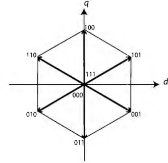
(18) CHAPTER 2. CONTROL TI-IEORETICAL BASIS. 15. boundaries. Lastly, .6..B(s) greatly depends on the arder :tnd characteristics of b¡(s) and bh(s). Thus, the margins over the Nichols chart can vary notoriously dueto relative small changes on the desired time-domain boundaries. Ali these problems are related to the initial design specifications. Consequently, there is no way to optimally derive a controller from QFT if B( s) is set under loase or arbitrary conditions. Most criticism about QFT has been directed to the imprecision of the loop-shaping process as well as its iterative nature. Automatic ways of tuning the C·Jntroller have been proposed as in [17] to avoid this complication. However, The dependence to B(s) still preclude QFT to find an optima! solution even if an automatic tuning method is used. Poss:ble solutions are to find an automatic way of defining B( s) or to propase a different way of placing Nichols chart 's magnitude margins. This last approach is the one used in this document.. 2.3 2.3.1. Direct Torque Control (DTC) VSI inverter and d-q transformation. Three-phase AC machines have replaced DC ones and have quickly and widely spread among diverse applications of electric drives dueto their advantages like improvement of energy efficiency and lmv maintenance requirements. Nevertheless, their speed is dominated by the AC fed frequency so its control can be seen as complicated when compared to that of DC motors, which can be directly modified by changing the input voltage. This made its use to be restricted to constant speed applications until a way to vary its input frequency was found, mostly thanks to developments in power electronics particularly far switching uses. Generally speaking, a power inverter is a device which can convert from a direct input voltage to an alternate output one. This conversion is achieved through the commutation of two semiconductors in series, connected between a DC bus. In arder to drive three-phase electric machines, three pairs of electronic devices are needed (one per phase). If ali semicond uctors are schematically represented as switches, a VSI connected to a motor woulc look like Figure 2.2. lt is easy to see that the whole three-phase VSI will have eight possible combinations, where six of them can drive current to the machine and two connects ali terminals to the same node. To represent the combination patterns in an easy way, a three binary digit notation can account far the state of the VSI at a given moment: Figure 2.2 shows a (100) combination, representing the first branch is connected to the bus' voltage, while the second and the third branch are connected to bus' reference..

(19) 16. CHAPTER 2. CONTROL THEORETICAL BASIS. Switching .--· device. Figure 2.2: VSI schematic representation V 100. _ __ _ _ _ _ _ _ 2Voc 3. -Voc 3. --------. 001. 010 011. Figure 2.3: Six-steps commutat'on pattern As the current can travel through the motor's windin.?;s on any direction depending on the VSI combination, the resulting output alternates, so convE,rting the DC input to an AC output. I t is evident that if the VSI is switched with a particular sequence (emulating a sinusoidal) the motor will rotate. Depending on the time each combinaticn is held, the emulated sinusoidal can vary its frequency and thus. vary the motor's speecl. Aforcmentionecl sequence will use thc six useful combinations of the VSI to delivcr six difh~rent threc-phase voltage levels. As a result. this techniquc is called six-steps commutation (depictcd in Figure 2.3). Those physical magnitudes related to the electric machinery operation cam he easily understoocl as rotating vectors if seen from the machine's front plate. The electric/magnetic contribution of those magnitudes can be seen as a two-dimensional vector projected transversally, dependent on the mechanical distribution of the phases. In arder to calculate such projections, the Clarke transform can he used (2.2)..

(20) CHAPTER 2. CONTROL THEORETICAL BASIS. 17. q 100. 011. Figure 2.4: d-q representation of VSI possible combinations. (2.2). If the VSI combinations shown in Figure 2.3 are mapped through (2.2), it is possible to see their rotating pattern on the newly generated d-q frame (Figure 2.4). The rotation corresponding to the commutation pattern shown before, should be taken counter-clockwise. ¼.hile the output voltage frequency can be modified easily, the emulated vültage magnitude cannot.. A different. problem arises when the applied voltage is delivered in squared steps so the current harmonics on the motor's phases would be high. Both issues directly depend on the un-modulated nature of the VSI combinations [104]. Nevertheless, this can be arnended through different commutation techniques.. 2.3.2. Modulation techniques. Carrier-based SPWM SPWM is based on modulation principie which translates a given signal to its equivalent average PWM representation through a high-frequency carrier. Resulting PWM varíes its duty cycle so voltage usage cluring a given time is increased or decreased. Overall averaging will resemble the original signal: however, its performance depends on the ratio between desired signal and carrier.

(21) CHAPTER 2. CONTROL THEORETICAL BASIS. 18. 41. "Cl. ::,. io E. <(. 41 "Cl. ~. a. E. <(. _ ___.____. o' - - - - - - ' - - - - ' - - - , . _ _ 0.1 0.15 o o.os. -'-_---'. 0.2. 0.25. 0.3. Time [s]. Figure 2.5: SPWM modulation technique for one single phase frequencies which is determined mostly by the hardware in which it is implemented. Additionally, the broadly described technique works for one phase only, so it needs to be partially triplicated so a three-phase VSI could be controlled. The central idea behind this technique is portrayed in Figure 2.5. There are many characteristics to notice form this figure; namely, carrier's frequency must be higher than the one of the desired signal so its important features are properly sampled into the PWM; carrier's frequency is the same of the resulting PWM while the desired signa! can be varied to meet application requirements; this method is highly dependent on the amplitude of both the desired signa! and the carrier. If carrier's amplitude is much higher than the sinusoidal wave, variations in duty cycle will be identical for the high and low states, so the combined effect of the thr,~e phases will be no different from the six steps technique. In comparison, whenever the carrier is smaller than the sinusoidal signa!, the PWM will stay on high or low state for more than one periocl. The relation between both mentioned magnitudes is called the modulation index. If this technique is to be implemented into a digital system, three different sinusoids phase-. shifted by 120º must be generated. There is only one carri,~r signa! needed as it can be shared far the three phases. The PWl\I signa! must be generated frorn the input/output management of the device by comparing all three signals towards the carrier, so deciding the state of the particular branch is a matter of comparing their magnitudes. Notice that the digital system, carrier, and sinusoid's frequencies are all different so the generation of the carrier and all three sinusoids time requirement must be met into the hardware timing capabilities..

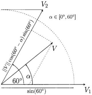
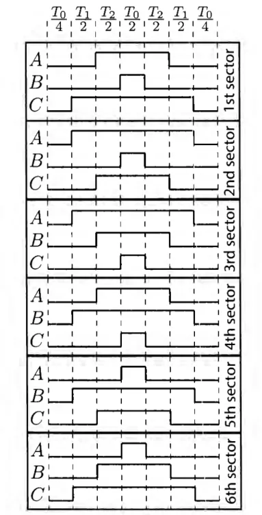
(22) 19. CHAPTER 2. CONTROL THEORETICAL BASIS. Voltage vector-based SVPWM Unlike the preceding technique, SVPWM [109] uses the g;raphical description of voltage vector combinations of the VSI as shown in Figure 2.4 to generate a rotating pattern. Any vector found in between a couple of VSI combinations can be generated by varying the time each of those two combinations is held on a time period; whenever the magnitude of the resulting vector is wanted to be lower, combinations (000) and (111) can also take sorne percentage of the period, thus reducing vcctor's magnitude. The combination of VSI vector voltages can deliver at most, a vector whose magnitude is restricted below the hexagon shown in Figure 2.4 so a complete circle can be fitted inside this restriction; this implies that even if the desired vector matches sorne standard VSI combination, the no-voltage combinations will be needed and the period will not be fully covered with a voltage vector. The PWM has a period itself Tpw Jtf so the vectors lirniting the sector in which the desired vector V is will have each a portian of that period, i.e. T1 and T2 . If the magnitude is different from the maximum possible, then a To will be also needed to apply the no-voltage vector, hence having Tpw,w =To+ T2 + T2. The proportion between T 1 and T2 can be derived from Figure 2.6: For a given angle. 0:. E [Oº, 60º] and considering that dueto restrictions imposed by the circumscribed. circle the maximum magnitude of the vector will be of sin(GOº) (for unitary. Vi,. V2 ), the projected. magnitude over the two vectors of the base will be within [O, sin(60º)], so equivalent equations can be provided to calculate both projection as (2.3).. TpwMIIVII cos(a: --'- 30º) T2. TpwMIIVII sin(a:). To. TpwJt1 - (T1 +T2:. (2.3). 1. Each time the whole period division is calculated, it must be applied to different VSI combinations depencling on the sector (6 VSI divisions conformecl by standard combinations) it is. The change between sectors is desired to happen smoothly, so symmetrical patterns must be followed for cach sector. If thcse divisions are enumerated orderly in CCW direction starting from the one placed directly over the positive d axis, the whole turn is rEpresented by Figure 2.7. In this way, there are two main parts of SVPWYI: timE calculation, and commutation assign-.

(23) CHAPTER 2. CONTROL THEORETICAL BASIS. 0:. 20. E. [Oº, GOº]. /V. sin(60º) Figure 2.6: Timing calculi derivation for SVPWM ment. Notice that the former needs two different trigonometric operations and a phase shift, while the last requires the input angle to be within a restricted interval and so, change each time the vector moves from one sector to another. The commutation patterns need to be assigned to each branch also depending on the sector so multiplexing is expec·;ed on implementation. However, this technique improves DC bus usage as V i:; moved guaranteeing the maximum timing combination for each standard VSI voltage vector whrn it touches the circumscribed circle. The method alone can not be over-modulated and dead times must be considered apart unless commutation includes not three but six patterns, two per phase, one per semiconductor.. 2.3.3. Traditional DTC. The coupled nature of induction motor makes impossible to control its torque and flux by clearly separated input variables as in the DC motor case. Both varia.bles are dependent on input voltage, while the speed is subjected to the input frequency of the AC voltage being fed. DTC enables decoupling of flux and torque by identifying the effect of thE voltage source inverter (VSI) combinations as voltage vectors in the d-q plane (Figure 2.2), so depending on the actual calculated position of the flux vector, each VSI combination would modfy the flux and torque in a directed manner. DTC first proposed by [100] provided a different way from Field Oriented Control (FOC) to achieve flux and torque decoupling through voltage and current sensors alone and a switching.

(24) CHAPTER 2. CONTROL THEOR.ETICAL BASIS. 1. A'. 1. 1. 1. 1. BI. 1. 1. 1. 1. 1. 1. 1. e~ 1. 1. 1. 1. 1. 1. 1. 1. 1. n. 1. 1. 1. 1. 1. 1. 1. L_;. '. i..... L~ ou. +-'. 1. 1. 1 1 QJ .¡....._....¡ V'I. +-' V'I. 'I"'"". 1. 1. 1. 1. 1. A~. 1 1. 1 1. 1 1. 1 1. B'. 1. 1. ~Bu. 1. 1. 1. 1. 1. 21. e: A~_J. 1. 1. B~. e~ 1. A~. 1. 1. 1. 1. 1. 1. 1. 1. 1 1. 1 1 1. 1 1 1. 1 1. 1. 1. 1. 1. 1. 1. 1. 1. 1. 1. 1. 1. B~. 1. 1. 1. 1. 1. 1. 1. 1. 1. 1. 1 1. 1-. B~. e' A'. 1. n. 1. 1. 1. IM. 1. 1. 1. 1. 1. 1. 1. 1. 1--. 1 1 1. 1. 1. 1. c~J. 1 1. n 1 1 1 1. ---1. i..... o +-' u. 1. 1. 1. 1. 1. --l~. 1. 1. 1. 1. 1. 1. 1. 1. 1. L~ ..e. 1. 1 1 1 1. 1. i..... L~ ..e. 1. 1. l.-. V'I. -o. 1. 1. 1. u. 1. 1. 1. 1. 1. 1. QJ. ~. 1 1. BI. ~~ 1. 1. i..... l~. 1. 1. 1. o +-'. 1. n n. -o e N. 1. 1. 1 1 1 1. 1. 1 ____,J. 1 1 1 1. 1. i..... 1 QJ _____¡ V'I. 1. L_;. 1. 1. 1. 1. 1. 1. 1. e: A'. n. 1. '. 1. QJ V'I. ~. i..... o. +-'. u. QJ V'I. 1. 1. ~. 1 1. 1. 1 1. 1 1 1 ---1 +-'. 1. 1 1 QJ 1 ----1 V'I. 1 1. 1. __J 1. i..... o u. L. 1-5. _J. \O. Figure 2.7: Sector dependent commutation patterns for SVPWM.

(25) CHAPTER 2. CONTROL THEORETICAL BASIS. 22 q. 100. d. 011. ' /. ''. '' ',. ''. 100 \. '. \\. Flux Hysteresis. Band 1. 1. lill-=:i------------~ Figure 2.8: DTC together with the VSI d-q graphical representations table subjected to hysteresis rules; this is, a whole simplification of the decoupling process became possible with good performance and fast response capabilities. After transforming voltages and currents onto the d-q plane through Clarke transform (2.2), torque and flux can be estimated through equations (2.4). A graphical approach to DTC is provided in Figure 2.8 where the flux vector position is clearly dependent on the VSI semiconductors combinations: in this way, the torque and flux can be increased, decreased, or remain unaltered depending on the error on both calculated quantities. Torque can be then increased by pulling the flux vector in the CCW direction while the flux itself by pulling it outwards the d-q plane.. (2.4). Depending on the error found on torque and flux, a voltag,~ vector is selected through a decision table which is also aware of the sector in which the flux vector is, so the modification imposed by the VSI combination is consistent with the desired effect. Figure 2.9 shows the decision scheme for torque regulation. Together with the flux bounding shown in Figure 2.8, the whole decision table can be generatecl (Table 2.1). If ali elements are placed together, an overall schematic view would be that of Figure 2 .10..

(26) CHAPTER. 2. CONTROL THEOR.ETICAL BASIS. 23. T. T*. 1. )t. Figure 2.9: Double hysteresis band representation for torque control. Wur. Tup. Wup. Thald. Wur. Tdo'tJm. Wdown. Tup. Wdown. T1ia1d. Wdown. Tdown. S1 (100) (000) (001) (110) (111) (011). S2 (110) (111) (101) (010) (000) (001). S3 (010) (000) ( 100) (011) (111) (101). :34 (011) (111) (110). (Cül) (COO) (100). S5 (001) (000) (010) (101) (111) (110). Table 2.1: Traditional DTC decision table. ~ a., Cl "'. ~ >. Figure 2.10: DTC shematic diagram. -e: a.,. ~. u. S6 ( 101) ( 111) (011) (100) (000) (010).

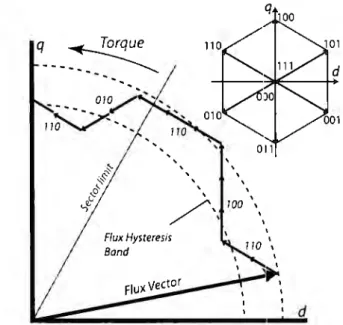
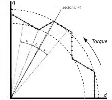
(27) CHAPTER 2. CONTROL THEORETICAL BASIS. 24. q. ---- ---. Sectorlimit. 1. 1. d Figure 2.11: Sector change known issues in to::que/flux degeneration Using the traditional DTC technique would yield to sorne known problems related to current harmonics, and torque and flux ripple. There is another cornmon issue related to torque stability when the flux vector is clase to the sector limits. Whenever the VSI vectors are applied as indicated in Table 2.1, the flux vector will behave differently depending on the specific zone it resides within a gi ven sector. Each VSI vector will take the same amount of time as tr.e decision process is supposed to be step-fixed discrete. Figure 2.11 shows three intervals (labeled as a, b, and c) where the same time is consumed and, however, the tracing speed of the circular path is deteriorated (b < a, b < e). The effect disparity of a certain vector's position, the eviden: ripple due to the hysteresis bands, the execution time of the algorithm, and the exclusive use of six-steps combinations are the reasons why the DTC, besides being a quick and easy direct control technique, delivers a poor performance for most applications. The technique discussed so far shows the traditional DTC approach; however, different topologies have been proposed to improve its performance, e.g. integrating a commutation technique like space vector PW~ (SVPWM) avoiding hysteresis band control or the decisions to be taken by a simple table, looking forward to achieve precise control over torque and flux..

(28) 25. CHAPTER 2. CONTROL THEORETICAL BASIS. T". t j.,,,,. Ol. ~ >. .,e: ~. u. Figure 2.12: SVPW?vI-DTC topology. q Sector Limit. ·-.:_-_.:-.. ___ '~arque. .. -. .. .', . ... ......... ......... .. '\. ~. '. .' ...'. /(\ \. Flux Reference. ~. :. :. d. Figure 2.13: SVPWM-DTC expected performance. 2.3.4. SVPWM-DTC. Thc SVPWM-DTC topology differs from the DTC traditional one in two main aspects: It uses controllers instead of hysteresis bands and a SVPW?vI modula,tion technique to replace the table with the predefined VSI voltage vectors (Figure 2.12). For this topology it is important to know the angle of the stator's flux vector instead of the sector so tbe voltage vectors sent to the motor compensates torque and flux magnitude errors adequately. The system's response will be time-dependent just like in the traditional DTC approach: however, as the vector is compensated for both, torque and flux, aforementioned problems related to sector boundaries are avoided. The flux vector response will be given as a soft curve instead of rigid vector combinations, which obviously will improve ripple and current harmonics. The normal SVPWM-DTC operation is shown in Figure 2.13..

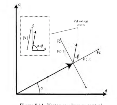
(29) CHAPTER 2. CONTROL THEORETICAL BASIS. 26. q. Figure 2.14: Vector quadrature control As the stator's flux and torque control can be achieved se¡::,arately by interpreting the effect of a certain voltage vector over the actual motor's state, individual controllers can generate a composite vector by modifying the magnitudes along a quadrature refenmce frame. The resultant vector will have, indeed, an angle and a magnitude which can be processed by the SVPWM technique. The preceding logic is depicted in Figure 2.14. The effect of the calculated vector over flux and torque is now independent to VSI combinations and sector-awarenes~:..

(30) Chapter 3. Robust control of a voltage buck converter through traditional QFT A DC/DC converter is a power electronics circuit used to modify the output characteristics of a DC source (voltage, impedance) at high efficiency and stable operation; it was first registered in 1978 by Lindmark [68]. A voltage converter is a time-variant system as its dynamical behavior depends on a switching device controlled through PW1I: moreover, the relation between the PW:VI duty cycle and the output voltage is not linear. Besides DC/DC converters have been successfully controlled in the past, it was until 90s when its non-linear characteristics where formally discussed and sorne advanced control techniques ,vere used to improve their performance. Nonetheless, the control objectives were met befare the system wa,s thoroughly understood as stated in [106]. The convenience of modeling them in a simplified manner has made researchers to follow this path too despite the neecl of two different models dependent on current conditions: continuous and discontinuous conduction modes (CCM and DCM).One of the most used methods to achieve linear representation of vcltage converters is the Small-signal state-space averaging [106]. Although simpler linear models allow the designer to consider well-known frequency-domain constraints and design techniques, its validity is restricted te, a determined bandwidth and can not attain non-linear behavior; as the linear model is desired to be kept simple, the control loop complexity must be increased through a more dependable con~roller [36]. This has lead to an increasing number of works related to control implementation under parametric variations, uncertain environments, and ambiguous measurements which commonly adopts one single control technique. 27.

(31) CHAPTER 3. QFT CONTROL OF A BUCK CONVERTER. 28. and a determined set of tests to validate converter's performance. The most commonly used control schemes are voltage mode control and current mode control [27]. The forrner takes the output voltage as its only feedback signal; however, its performance degrades on DCM. The current mode control effectively alleviates the sensitivity of the converter dynamics and could offer near uniform loop gain characteristics for both CCM and DCivl operation. The key feature of current-mode control is that the inner loop changes the inductor into a voltagedependent current source at frequencies lower than crossover frequency of the current loop. A commonly used way to implement a current mode control is using two Proportional Integral (PI) controllers; one for the inner current loop and one more for the outer voltage one. In this chapter, the LQR approach is employed to tune it. The algorithm proposed for PI/PID controller tuning via LQR approach and selection criteria of the Q and R matrices were taken from [65, 66]: this approach aims to control PWM-type switching DC-DC converters independently frorn their circuit topologies and open-loop pole-zero locations [65]. Different optimization iterative methods have been used for this same purpose like in [20] and they ,::an also be used to automate the QFT design process. This makes the actual comparison to target controllers natural complexity (number of pales and zeros). QFT approach has been also used for voltage converters. It allows the designer to quantify how demanding a set of plants are in terms of further control design, to deal with uncertainties and disturbances, and to set the problem in comrnonly ·1sed frequency-domain equations [87]. These characteristics seem to suit perfectly to a linear model as the one introduced befare. QFT technique has been effectively used for voltage converters control as in [4, 7, 88, 89, 96]: however, its use is not popular and little literature can be found about specific problems. Robustness is commonly adclressed through fuzzy and sliding-rnode approaches [36, 77, 28, 102]. Furthermore,. H 00 optimizatíon can also be used as in [39] where the PID perspective is also outperformed. The QFT approach presented here can partially complement the comparison study presented in [93], devoted to robust control over CUK converters. Further research would clarify /extend this comparison to include QFT specifically towards the µ controller, reported to outperform H 00 and fuzzy ones. This chapter shows a parallel PI-LQR and QFT design, and tests them under varying load and input voltage conditions. A comparison between PI and QFT controllers has been presented in [49] but the design process is not completely covered or explained, and the PI tuning is made mostly arbitrarily. In addition, controllers are designed only for voltage mode so no conclusions about.

(32) 29. CHAPTER 3. QFT CONTROL OF A BUCK CONVERTER Vour. R D VIN. Figure 3.1: Buck converter circuit dynamical tracking, output ripple, and rising times are offered beyond overshoot comparison.. 3.1. Small-signal state-space averaging. This method aims to describe the dynamics of the converter as a group of time-invariant equations which are valid for the whole commutation cycle [83]. Final results are obtained based on the smallsignal transfer function so their validity is restrained to relati vely small voltage or load perturbations [75]. However, it is very adequate for analysis in both stable and transient states, and is now considered an essential design tool for component selection and control achievement for a particular group of specifications [75]. In order to obtain a mathematic:al model, a state-space representation of the circuit is attained through (3.1), given that at eac:h stage of commutation (open/closed switch) the circuit is linear and time-invariant. This means that during each time sub-interval. the system can be desc:ribed by a group of differential ordinary equations which c:omply with the energy conservation laws [95]. The exact description of the system is obtained by averaging the state variables acquired at each state. While the averaging eliminates the variation in time for the whole commutation cycle. it <loes not linearize the model, making the small-signal assumptic-ns to be necessary. This considers the circuit feedback to be disabled while a perturbation (with DC and AC components) is added at the voltage input. then a frequency analysis is driven. Resulting non-linear function is approximated by Taylor series to its second term. Finally, superposition allows only the DC components to be considered solutions to the equation. A detailed description of this process can be found in [19].. If the preceding method is applied to the buck converter shown in Figure 3.1 under CC:ívl, (3.1) and (3.2) can be derived as current and voltage transfer f:mctions respectively, according to the duty cycle. The same technique under DCM delivers the transfer function shown in (3.3) and (3.4).

(33) 30. CHAPTER 3. QFT CONTROL OF A BUCK CONVERTBR. Symbol. Description Input Voltage Inductor Capacitar Load PWM Period PWM Duty cycle toN switch resistance Inductor resistance Capacitar resistance. V¡N. L. e R Ts D Ts. TL. re. Value 24V 300µH 220µF 12n lOµs 1 0.01n 16.3mD 0.305D. Table 3.1: Physical parameters used far model calculation far current and voltage respectively.. =. G· (s) iD. A= (L. (.s(CR+Crc)+l)Vuv CLRs2+As+R+r1.+r,. + CRrL + C(Rrs + rc[R + Ls + TL + r. (s) _. G VD. -. A= (R B = (R. VIN*Rrc(s(CR+C,·c)+l) As 2+Bs+(R+rc)(R+rL+r,). (3.1) 5 ])). (3.2). + rc)(CLR + CLrc). + rc)(L + CRrc + CrcrL + Crcrs + CR(rL + r 8 )). (s). G iD. G. VD. =. (s) -. A. 2V1 N(l/CR+s) CL ( 8 2 A 4(2-2/B) ) ' + s+CDRT8 B(l-2/B)2. CL(s2+As+. = ( 'tR + B = 1+. 2 V¡N 4(2-:!/B) ) CDRT.,B(l-2/8)2. DT., B(i-2/ B)). V1 +. 0. f. ~r.:. (3.3) (3.4).

(34) 31. CHAPTER 3. QFT CONTROL OF A BUCK CONVERTER. ;--------i --.,. r..,.,'.JC¡llrG,. (•l =I K. )'(I). =I. Figure 3.2: PID loop controller. 3.2. PID tuning through LQR approach. The LQR tuning technique was selected as a reference bE-cause it is a reliable and widely used approach around PI usage. So, further evaluation and comparison is possible towards different methods and conclusions can be elaborated from salid foundations. PI tuning through trial-error or parameter adjustment dependent on fractional arder is completely avoided in this work. Using the Lyapunov's method, the LQR design problem reduces to the Algebraic Riccati Equation (ARE) which is solved to calculate the state feedback gdn for a chosen set of wcighing matrices that regulate the penalties due to state variables and control signa! trajectories deviations. The method used to obtain Q and R matrices was genetic algorithms (GA) as used by [92] while the performance index was taken from [65, 66].. (1~6. Q. R. o (3.5). 0.025e - 2. o. (0.001). Consider a linear process described by standard state-space representation. ±( t). Ax(t). y(t). Cx(t). + Bu(t). (3.6). and X1 =. J. e(t)dt,. X2 =. e(t),. X3. =. de(t). -;¡¡-·. (3.7).

(35) 32. CHAPTER 3. QFT CONTROL OF A BUCK CONVERTER From the block diagram of Figure 3.2,. -E(s) U(s). s2. K +as+b. (3.8). thus, equations turn into. [s 2 +as+ b]E(s). = -Ku,. (3.9). which can be written in the time domain as. e+ ae +be= -Ku.. (3.10). Substituting (3.7), (3.10) can be rewritten as. (3.11). so the state space formulation becomes. X]. : 1. ~ ~ 11 :~ 1 1: 1. O -b. +. -a. x3. (3.12). u.. -K. In order to have a LQR formulation of (3.6) the cost function (3.13) is minimized.. (3.13) Its result provides the state feedback control law as stated in [85] u(t) = -R- 1 ET Px(t) = -Fx(t),. (3.14). where P is the symmetric positive definite solution of the Continuous ARE:. AT P. + PA -. PER- 1 ET P -t- Q. = O.. (3.15). The weighing matrix Q is symmetric positivc semi-definitc and the factor Risa positive number.. If the plant's transfer functions are used on (3.12), A and E matrices can be derived: in addition to matrix Q from (3.5) and coefficient R from (3.6), preceding; values can solve matrix P form (3.15).

(36) CHAPTER 3. QFT CONTROL OF A BUCK CONVERTER. 33. through an optimization algorithm. As a standard (usual) consideration, if the solution for P is considered to be unique, the state feedback gain matrix becomes (3.17), corresponding to the optimal control signal.. F. (3.16) XI ( t). - [ -K¡. K¡. J. -Kp. e(t)dt. KD ]. x2(t). X3(t). + Kpe(t) + KD de({~ dt. therefore,. K¡ Kp KD. 3.2.1. (3.17). =. kP23/R kP33/R.. Specific design for Buck converter. The parameters shown in Table 3.1 are those of a real converter. If they are substituted, CCM equations can be obtained as (3.18) and (3.19), while DCM ones as (3.20) and (3.21).. GiD(s) GvD(s) GiD(s) GvD(s). s + 2.95e7 s 2 + 1415.19s + l.47e7 s + 3.54e8 2 s + 1415.19s + l.48e7 s + 7.57e4 2 s + 4.0le7s + 3.09e9 -l.54el:. 2 211.77s + 2.37e7s + 2.29e10. (3.18) (3.19) (3.20) (3.21). Coefficients from preceding equations are substituted in (3.12) so A and B matrices of the ARE.

(37) 34. CHAPTER 3. QFT CONTROL OF A BUCK CONVERT.ER Parameter Current mode. Value. Kp K1. 20.8593 63244.6. Voltage mode. Kp K1. 2.90115 7071.06. Table 3.2: Resulting PI coefficients due to LQR tuning are obtained as follows:. A. O. 1. o. o. O -1.47e7. B. [. (1. 1. (3.22). -14~5.19. _3L,8. By substituting the values in equations (3.22),(3.5), and (3.6) and solving (3.15) the following matrix P is obtained: 415.81 P ==. 0.036 3.98e - 7. 0.0363. 3,.98e -. 71. 14.74e - 6 1 63e - 10 l.63e - 10. (3.23). 1 43e - 14. By using (:3.23) on (3.17), the PI tuning coefficients are derived. Results are shown on Table 3.2.. 3.2.2. QFT design for buck converter. The uncertain model to use as input to QFT controller design is obtained by varying the voltage input parameter from 20V to 30V and the output load from l..2D to 60D. As many other techniques, QFT design must be aware of the two different modes the Buck converter can operate: CCM and DCM [4]. For sake of convenience, a controller for CCM operating mode will be designed based on the following uncertain transfer function (3.24), obtained through the variations discussed above. V(s). D(s). s2. [l.62e4, 3.03e4]s + [2.4le8, 4.52e8] + [1.14e3, 3.88e3]s + [l.22e7, l.50e7]. (3.24).

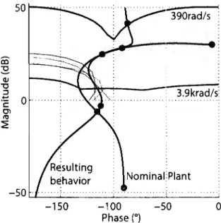
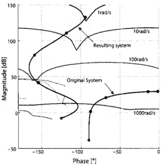
(38) 35. CHAPTER 3. QFT CONTROL OF A BUCK CONVERTER 60. 40. ce. ~ 20f ~. i. ::,. li. .'!:. O'. e C'l ro. ~. --20 --4~. º-', -.------,~º_:,_ Frequency (rad/s). Figure 3.3: Open loop Bode plot for sorne plants contained in (3.24) Equation (:3.24) relates the input duty cycle to the oucput voltage; in this case, the current rnodels are ignored and a single voltage loop is assumed instead of a cascade control approach. Current control is known to alleviate sensitivity to system d:mamics [55] and to provide an effective way to limit the output current [88], so a voltage controller is expected to present high output ripple. Current control mode will be covered later; however, voltc:,ge mode controlled systems have also been reported like in [4], presenting good results. According to the dynamic response of the systems contained in (3.24), a settling time of lms can be achieved so the tracking boundaries are defined to fulfill this specification as (3.25). As the QFT approach will ensure that the magnitudes difference along the whole bandwidth will be constrained to those imposed by the boundaries, it is importa,nt to detect those frequencies at which the set of plants perform different. Figure 3.3 shows that the main variation occurs at 3.9krad/s, so the set of test frequencies can be chosen to be [390, 3.9k, 39k]rad/s.. b1 (s). 2.95e09 s 2 + 5.40e5s + 2.95e09 l.48e12 3 2 s + 63.60e3s + 5.89e08s. (3.25). + l.48e12. Under the aforementioned conditions, the QFT design can proceed to find the tracking boundaries. In addition, the noise rejection specifications are also considered to always be bellow ldB. The resulting margins and the nominal plant 01 are shown in Figure 3.4. In order to make the resulting behavior of LA (s) to be consistent to the margins, different actions.

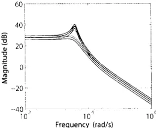
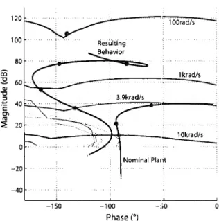
(39) CHAPTER 3. QFT CONTROL OF A BUCK CONVERTER. 36. • 3.9krad/s:. -150. -100. Phase (º). -50. o. Figure 3.4: Open loop and controlled nominal plant Nichols chart for CCM must be taken. A pole at zero must be added to reach the lowest frequency margin along with two pole-zero pairs to border the sensitivity boundaries. The loop shaping, in this case, delivered the result shown at Figure 3.4 which fully meets the desired performance by using (3.26). Resulting plant's trajectory over Nichols chart presents a phase margin of 54.6º, and infinite magnitude margin. G(s). =. 2. 5.44e12s + 5.44e16s 2.le07s 3 + 3.675e12s 2. + 1.142e20 + 7.875e16s. (3.26). The last part of the design implies the incorporation of e, pre-filter (3.27) to fit the set of plants within the desired boundaries: moreover, the correct operation of the controlled system has been evaluated towards a discrete set of frequencies, so a comple;e spectral view is needed to confirm a reliable design. Hence, a bode plot is obtained from the resulting loop. Results are shown in Figure 3..s.. F(s) =. 3450. s. + 3450. (3. 27). The current mode control must be derived from a set of plants which relates the control input as a duty cycle to the output current as (3.28). This set o: plants were obtained under the same uncertain conclitions than the voltage mode case: however, the implications of these plants are totally different as they can naturally rise to its setting point in about 0.3ms. In this way, the boundaries can not be the same and must be redefined..

(40) CHAPTER 3. QFT CONTROL OF A BUCK CONVERTER. e. 37. -9o·. (IJ. V,. 1-180 · c.. 10~ Frequency (rad/s). 10 6. Figure 3.5: Resulting Frequency response after applying QFT controller. I(s) D(s). s2. [0.66e5, le5]s + [ü.05e8, 3.02e8] + [l.14e3, 3.88e3]s + [l.22e7, l.5e7]. (3.28). Expected boundaries are constructed so a step response reaches a settling time around 0.4ms as shown in (3.29). The dynarnical implications of this restriction modification confirms the expected improvement in dynamical tracking if compared towards vo.tage mode controller; nevertheless, an additional controller will be needed to complete the cascade outer voltage loop (This is performed la ter in this chapter). For this particular case and based on Figure 3.6, the selected frequencies are [100, le3,3.9e3, 10e3,30e3] rad/s.. l.155e10 + l.lle06s + l.15eJ.0 9.07e12 3 2 s + 87e3s + l.65e095 + 9.07e12. s2. (3.29). Considering both, the tracking boundaries imposed by (3.29) and assuming a noise rejection threshold of ldB, the Nichols chart can be plotted so the original 01 development of the nominal plant is analyzed (Figure 3.7). It can be seen that a controller similar to the one used on voltage mode control is required as the plant needs to fulfill a very 3imilar trajectory. After loop shaping through a pole at zero and two pole-zero pairs, the resulting controller can be derived as (3.30), and its related pre-filter as (3.31). The resulting phase margin is of 74.3º and again, an infinite magnitude margin is achieved..

(41) 38. CHAPTER 3. QFT CONTROL OF A BUCK CONVERTER. 4(1. 30. -1 o ~ ~ - - ------· 1ff' 10' 10'. ----·----·- -·-·---------------·. 10· Frequency (rad/s). 10'. 10'·. Figure 3.6: Open loop Bode plot for sorne plants contained in (3.28). 120. 100rad/s. -. 100 80. co. :!:!. 60 QJ. "C. -~e:. 40. en. n:,. ~. 20. -150. -100. -SO. o. Phase (º). Figure 3.7: Open loop and controlled nominal plant Nichols chart for CCM.

(42) CHAPTER 3. QFT CONTROL OF A BUCK CONVERTER. 39. ',(). 1O Frequency (rad/s). 10 -. Figure 3.8: Resulting frequency response after applying QFT controller. G(s) = l.92e14s 2 + l.82e18s l.75e07s 3. F(s). + 3.36e21 + l.75el3s 2 + 1.4e15s. =. 7800 s + 7800. (3.30). (3.31). Besides more frequencies were taken this time to analyze tracking and sensitivity boundaries. a continuous frequency sweep is needed to see if the controlled loop together to the pre-filter are able to fulfill the boundary requirements. The resulting Bode plot is shown in Figure 3.8 where it is clear that the boundaries are respected along the whole frequency span.. 3.3. Incorporation of voltage through cascade QFT design. Different techniques to attain a cascade-QFT controller has been already presented by Horowitz himself as pointed by Wu and Jayasuriya [119]. This last c:ited work actually includes a simplification which permits the cascade loops to be processed through their sensitivity transfer function alone. A different approach is taken here assuming the already controlled current loop to be the plant itself. However, no analytical procedure was taken and instead, an identification technique was used to simplify the problem by its approximate uncertain models. There are evident trade-offs when using an identification method. The resulting set of systems will be of a pre-defined topology, and system's complexity will be embedded in the resulting model without making any particular effort to fit it.. However, results can be imprecise and specific. considerations about system's nature can be missed, leading to unexpected results and performance failures. The templates' construction of the QFT methodology allows sorne of these unconsidered.

(43) CHAPTER 3. QFT CONTROL OF A BUCK CONVERTER. 40. Figure 3.9: Block representation of buck converter cascade control topology defects to be absorbed, whether they stay inside templates' b::mndaries. This last assumption is not fortuitous and can be closely related to the effectiveness of the identification as presented by Chen, et al. [14]. This last cited work presents an identification me·:hod which delivers an uncertain plant through a nominal plant, bounded noise, and bounded unc,~rtainty. The validity of the resulting model is also subjected to the available information, and can group unconsidered plants found within the tolerance boundaries. The considered topology is shown in Figure 3.9, where the previously designed controller has been surrounded by a simple dashed line. A set of identified models is taken from the input of the current pre-filter to the voltage output of the buck converter. The inner current loop is also considered inside this equivalent voltage source. The QFT design can proceed normally once the uncertain plants have been obtained. In this work, the least squares non-parametric identification technique was used. Eight open loop tests were performed over the buck converter; each one forced the system to reach lOV by selecting an appropriate setting point. The load was varied over the values [1.2, 2.1, 3.7, 6.4, 11.2, 19.6, 34.3, 60.0]0. Results delivered a continuous model conformed by no zeros and one pole, after converting it from its original discrete version through the zero-order-hold method. Identified uncertain system is shown in (3.32).. G. 8. =. e( ) ·. 3.3.1. [3237, 2369] S. + [54.78, 1971]. (3.32). Specific design for buck converter. The presented buck topology together with the QFT current control behave as a current source. The output capacitar and the load itself forman RC circuit with first-order nature. In the preceding sections, the pre-filter was designed to attain a desired step-response performance and consequently, to limit controller's effort. However, for the cascade perspei::tive, the current variations should be subjected to expected tracking of the voltage signal..