Road freight transport, logistics and co2 emissions: case study of Tabasco, Mexico

Texto completo

(1)BE. BENEMÉRITA UNIVERSIDAD AUTÓNOMA DE PUEBLA FACULTAD DE ECONOMÍA MAESTRIA EN ECONOMÍA. ROAD FREIGHT TRANSPORT, LOGISTICS AND CO2 EMISSIONS: CASE STUDY OF TABASCO, MEXICO. T. E. S. I. S. PRESENTADA PARA OBTENER EL TÍTULO DE MAESTRÍA EN ECONOMIA P. R. E. S. E. N. T. A. ITZCOATL ANGELES TAH COMITÉ DE TESIS DR.YVES DANIEL BUSSIÈRE (BUAP) DR. CHRISTOPHE RIZET (IFSTTAR) DR. SALVADOR PEREZ MENDOZA DR. ENRIQUE BUENO CEVADA PUEBLA, PUE.. AGOSTO 2016. I.

(2) I thank first my parents and friends, who have given all the effort to help me finish this stage of my life, and thank them for supporting me in all the difficult moments of my life such as happiness or sadness, they have always been with me and thanks to them, I am what I am now and with the efforts of them and my effort can now be a great professional and will be a great pride for them and for all those who trusted in me. I also thank my professors who always trusted in me and helped me in my academic life of this Master, and also important to thank CONACYT for my scholarship that let me study and research, VIEP to support my investigation travels and the administration of the Master in Economic at BUAP, which always helped me in my academic life and research stays. Finally but not least important, I thank the Government of the state of Tabasco, SCT and the firm LOGIT of Puebla help me with all the information and statistics for my research.. II.

(3) Master´s Thesis at the Faculty of Economics of the Benemérita Universidad Autónoma de Puebla (BUAP) Road Freight Transport, Logistics and CO2 Emissions: Case study of Tabasco, Mexico by Itzcoatl Angeles Tah Co-directors: Yves Daniel Bussière (BUAP); Christophe Rizet (IFSTTAR) 2016 Salvador Perez Mendoza (BUAP); Enrique Bueno Cevada(BUAP). Transport is an important source of CO2 emissions, around 30% in developed countries and 20% in many emerging countries, such as Mexico. In European cities, the part of freight transport in transport-related CO2 emissions is estimated at 25%, a third of transport-related NOx and half of transport-related particulate matter (Rizet & Dablanc, 2014). The objective of this thesis is to study to what exlatent technological choices and improvement in logistics can reduce CO2 emissions in the transportation of goods in Mexico, based on the case study of Tabasco where recent data (2014) was made available by the Government of the State of Tabasco, and the consulting firm LOGIT of Puebla, for academic purposes. The main source of data are 1- A road survey with a large sample in the Eastern axis of Mexico of freight transport indicating the type of transport, the type of merchandise, its origin and destination. Preliminary results show that around 50% of trucks travel empty when a satisfying level would be closer to 15%. Based on this case study, the objective is to analyze how different kinds of freight transport have a different effect on the production or emissions of carbon particles into the environment, also find feasible ways to reduce CO2 emissions by improving technology (type of vehicle, type of fuel, ....) and by a better logistic to optimize the supply and demand chain in the transportation of goods.. III.

(4) Road Freight Transport, Logistics and CO2 Emissions: Case study of Tabasco, Mexico Index of contents 1. Chapter I: Introduction. a. Background b. Objectives. c. Instruments to use. d. Methodology.. Page 1 1 11 11 12. 2. Chapter II: The best methods of logistics in the world (Road freight transport). a. Europe (EU) b. America. 17. 3. Chapter III: Logistics, road freight transport in México and its problems. a. Logistics of road freight transportation in México. b. Common problems of freight transportation in México.. 28. 4. Chapter IV: Method to calculate carbon emissions. a. Variables to use to calculate carbon emissions. i. Description of data to use for the calculation of carbon emissions. ii. Methods used to calculate variables for calculation of carbon emission. b. Calculation and result of carbon emissions.. 40 40 40. 5. Chapter V. Interpretation of LOGIT statistics, case Tabasco. a. Variables to use to calculate carbon emissions. b. Behaviour of the freight transportation, case Tabasco. c. Behaviour of the carbon emissions in the case of Tabasco. d. Behaviour of the application of the low price of carbon emission. e. Behaviour of the application of the high price of carbon emission.. 57 57 63 83 92. 6. Chapter VI. Synthesis and final considerations.. 94. 19 23. 29 38. 52 53. 92. IV.

(5) 7. References. Index of tables. 101 Page. 1. Chapter I: Introduction. Table I.1 Contaminants in fossil fuels. 1. Table I.2 : Fuels in México, 2014. 5. Table I.3 Methodologies to calculate CO2 in México. 12. 2. Chapter II: The best methods of logistics in the world (Road freight transport). Table II.1. Criteria for the road transport companies, 2011.. 20. Table II.2. Distribution of modal of land freight transport (% of Tons-. 23. Kilometres Table II.3.Federal Commercial Vehicle Size Limits on the National Network. 24. Table II.4. Distribution of the freight transport in USA, 2011.. 25. Table II.4. Heavy Truck Weight and Dimension Limits for Interprovincial. 26. Operations in Canada. 3. Chapter III: Logistics, road freight transport in México and its problems. Table III.1. Total exportations and importations by classification of transport,. 28. 2006 and 2015. Table III.2. LPI per study area in México.. 29. Table III.3. Principal corridors of road freight transport, 2014 (Average of. 33. tons per day) Table III.4.a Classification, Maximum length and weights of road freight. 35. transport vehicles (México, 2014) Table III.4.b Classification, Maximum length and weights of road freight. 36. transport vehicles (México, 2014) Table III.4.c Classification, Maximum length and weights of road freight. 37. transport vehicles (México, 2014) V.

(6) 4. Chapter V. Interpretation of LOGIT statistics, case Tabasco. Table IV.1.1. Classification and weight of the cargo. 41. Table IV.1.2. Classification and weight of the cargo. 42. Table IV.3. During the week. 44. Table IV .4. Type of Transport on Weekends. 45. Table IV.5. Important and must used destinations during the week. 46. Table IV.6. Important and most used Destinations on weekends. 47. Table IV.7. Age of the transport vehicle during the week in %. 48. Table IV.8. Age of the transport vehicle during weekends in %. 48. Table IV.9. Weight of the cargo during the week in %. 50. Table IV.10. Weight of the cargo during. 50. Table IV.11. Empty percentages.. 51. Table IV.12. Data for Examples. 53. Table IV.13. Summary of CO2 emissions (Tons). 56. 5. Chapter V. Interpretation of LOGIT statistics, case Tabasco. Table V.1 Balance of Inter-Regional Transportation During the Week, in. 58. percent of the difference between Origin and Destination. Table V.2 Balance of Inter-Regional transportation on weekends, in percent of. 59. the difference between Origin and destiny. Table V.3 Principal corridors used during the week in %. 60. Table V.4. Main corridors used on weekends, in %. 62. Table V.5. Balance of inter-regional transport of 2 axes, during the week.. 64. Table V.6. Most used corridors, 2 axes, during the week.. 64. Table V.7. Empty travels, 2 axes, during the week.. 64. Table V.8. Balance of inter-regional transport of Pick-ups, during the week.. 65. Table V.9. Most used corridors, Pick-ups, during the week.. 65. Table V.10. Empty travels, Pick-ups, during the week.. 65. Table V.11. Balance of inter-regional transport of 3 axes, during the week.. 66. VI.

(7) Table V.12. Most used corridors, 3 axes, during the week.. 66. Table V.13. Empty travels, 3 axes, during the week.. 66. Table V14. Balance of inter-regional transport of 4 axes, during the week.. 67. Table V.15. Most used corridors, 4 axes, during the week.. 67. Table V.16. Empty travels, 4 axes, during the week.. 67. Table V.17. Balance of inter-regional transport of 5 axes, during the week.. 68. Table V.18. Most used corridors, 5 axes, during the week.. 68. Table V.19. Empty travels, 5 axes, during the week.. 68. Table V.20. Balance of inter-regional transport of 6-9 axes, during the week.. 69. Table V.21. Most used corridors, 6-9 axes, during the week.. 69. Table V.22. Empty travels, 6-9 axes, during the week.. 69. Table V.23. Balance of inter-regional transport of 6-9 axes, during the week.. 70. Table V.24. Most used corridors, Double trailer, during the week.. 70. Table V.25. Empty travels, Double trailer, during the week.. 70. Table V.26. Summary of the important results, during the week. 72. Table V.27. Balance of inter-regional transport of 2 axes, weekends.. 73. Table V.28. Most used corridors, 2 axes, weekends.. 73. Table V.29. Empty travels, 2 axes, weekends.. 73. Table V.30. Balance of inter-regional transport of Pick-ups, weekends... 74. Table V.31. Most used corridors, Pick-ups, weekends.. 74. Table V.32. Empty travels, Pick-ups, weekends.. 74. Table V.33. Balance of inter-regional transport of 3 axes, weekends.. 75. Table V.34. Most used corridors, 3 axes, weekends.. 75. Table V.35. Empty travels, 3 axes, weekends.. 75. Table V36. Balance of inter-regional transport of 4 axes, weekends.. 76. Table V.37. Most used corridors, 4 axes, weekends.. 76. Table V.38. Empty travels, 4 axes, weekends.. 76. Table V.39. Balance of inter-regional transport of 5 axes, weekends.. 77. Table V.40. Most used corridors, 5 axes, weekends.. 77. Table V.41. Empty travels, 5 axes, weekends.. 77. VII.

(8) Table V.42. Balance of inter-regional transport of 6-9axes, weekends.. 78. Table V.43. Most used corridors, 6-9 axes, weekends.. 78. Table V.44. Empty travels, 6-9 axes, weekends.. 78. Table V.45. Balance of inter-regional transport of double trailer, weekends.. 79. Table V.46. Most used corridors, double trailer, weekends.. 79. Table V.47. Empty travels, double trailer, weekends.. 79. Table V.48. Summary of the important results, weekends. 81. Table V.49. Carbon emissions per year (Tons), during the week.. 83. Table V.50. Summary of the important results, weekends. 83. Table V.51. Resume of analysis of CO2 emissions, distances and weight of. 91. the cargo, case of Tabasco 2014. Table 5.52. Application of 20 Dls prices emissions, during the week. 92. Table 5.53. Application of 20 Dls prices to CO2 emissions, weekend.. 92. Table 5.54. Application of 40 Dls prices to CO2 emissions, during the week.. 92. Table 5.55. Application of 40 Dls prices to CO2 emissions, weekends.. 93. 6. Chapter 6. Synthesis and final considerations Index of graphics 1. Chapter I: Introduction. Graphic I.1. The greenhouses gases, México, 201 Graphic I.2. Gas Production. México, 2014. Graphic 1.3. Distribution of Freight Transportation around the world. Graph I.4: Pollution of the fuels in México (CO2), 2014 2. Chapter II: The best methods of logistics in the world (Road freight transport). Graphic II.1: Distribution of the freight transportation in EU, 2010 Graphic II.2: EU road freight transport by type of operation in 2010 Table II.3.Federal Commercial Vehicle Size Limits on the National Network 3. Chapter III: Logistics, road freight transport in México and its problems. Graphic III.1. Exportations of NAFTA by classification of freight transport (% percent of the total). Page 3 4 5 6. 20 22 24. 30. VIII.

(9) Graphic III.2. Importations of NAFTA by classification of freight transport (% percent of the total. Graphic III.3. Curve of road transport cost, (Inside the countries, kms-Dollars) Graphic III.4. Classification of vehicles and percentages of the total of vehicles in Mexico, 2010 4. Chapter V. Interpretation of LOGIT statistics, case Tabasco. Graphic IV.1 Type of Transport during the week Graphic IV.2. Type of Transport on weekends Graphic IV.3. Age of transport during the week Graphic IV.4. Age of transport vehicles on weekends Graphic IV.5. Weight of the cargo during the week Graphic IV.6. Weight of the cargo on weekends in % Graphic IV.7. Empty travels, during the week Graphic IV.8. Empty travels, on weekends 5. Chapter V. Interpretation of LOGIT statistics, case Tabasco. Graphic V.1 Balance of Inter-Regional transportation during the week, in percent of the difference between Origin and destiny. Graphic V.2 Balance of Inter-Regional Transportation on Weekends, in percent of the difference between Origin and destiny. Graphic V.3 Principal corridors used during the week (Number of times used in the period) Graphic V.4. Main corridors used on weekends, (Number of times used in the period) Graphic V.5. Type of cargo, 2 axes, during the week. Graphic V.6. Type of cargo, Pick-ups, during the week. Graphic V.7. Type of cargo, 3 axes, during the week. Graphic V.8. Type of cargo, 4 axes, during the week. Graphic V.9. Type of cargo, 5 axes, during the week. Graphic V.10. Type of cargo, 6-9 axes, during the week. Graphic V.11. Type of cargo, Double trailer, during the week Graphic V.12. Age of vehicles during the week. Graphic V.13. Type of cargo, 2 axes, during the week. Graphic V.14. Type of cargo, Pick-ups, during the week. Graphic V.15. Type of cargo, 3 axes, during the week. Graphic V.16. Type of cargo, 4 axes, during the week. Graphic V.17. Type of cargo, 5 axes, during the week. Graphic V.18. Type of cargo, 6-9 axes, during the week. Graphic V.19. Type of cargo, Double trailer, during the week. 31 32 34. 45 45 48 49 50 50 51 52. 59 60 61 63 64 65 66 67 68 69 70 71 73 74 75 76 77 78 79 IX.

(10) Graphic V.20. Age of vehicles during the week. Graphic V.21. Resume of behavior, 2 axes: LOG CO2 emissions VS LOG weight of cargo and distance (Case of Tabasco, 2014) Graphic V.22. Resume of behavior, pickups: LOG CO2 emissions VS LOG weight of cargo and distance (Case of Tabasco, 2014) Graphic V.23. Resume of behavior, 3 axes: LOG CO2 emissions VS LOG weight of cargo and distance (Case of Tabasco, 2014) Graphic V.24. Age of vehicles during the week. Graphic V.25. Resume of behavior, 5 axes: LOG CO2 emissions VS LOG weight of cargo and distance (Case of Tabasco, 2014) Graphic V.24. Resume of behavior, 4 axes: LOG CO2 emissions VS LOG weight of cargo and distance (Case of Tabasco, 2014) Graphic V.25. Resume of behavior, 5 axes: LOG CO2 emissions VS LOG weight of cargo and distance (Case of Tabasco, 2014) Graphic V.26. Resume of behavior, 6-9 axes: LOG CO2 emissions VS LOG weight of cargo and distance (Case of Tabasco, 2014) Graphic V.27. Resume of behavior, double trailer: LOG CO2 emissions VS LOG weight of cargo and distance (Case of Tabasco, 2014) Chapter VI. Synthesis and final considerations. 80 84 85 85 86 87 85 86 87 87. X.

(11) Chapter I: Introduction.. A.

(12) Road Freight Transport, Logistics and CO2 Emissions: Case study of Tabasco, Mexico I.- Chapter I: Introduction. a. Background Like many other countries, developing and emerging countries in particular, México has to face many problems. Corruption, poverty, and bad use of public spending are some of them; on top of that, Mexico is also affronting the climate change challenge. The objective is to limit the average world temperature increase to 2º C. However, we are already experiencing different effects related to temperature rising in our environment, such as ice melting, the rising of sea levels and land erosion. Such effects produce climate changes variations reflected in droughts, loss of crops and death of animals in different parts of the world which directly affect humankind and our food needs. At this moment the level of pollution is high. According to The World Bank, México is producing 3.9 metric tons per capita of CO2 as well as other contaminants. Table I.1 Contaminants in fossil fuels Gas. CO. HC. NOx. CO2. CH4. EF g/litre. 117.69. 13.75. 9.03. 2,081.7. 0.72. Source: René Rodríguez Lara, Jorge Raúl Gasca Ramírez, Luis Leobardo Díaz Gutiérrez . (Agosto 2014). “FACTORES DE EMISIÓN PARA LOS DIFERENTES TIPOS DE COMBUSTIBLES FÓSILES QUE SE CONSUMEN EN MÉXICO”. Dirección de Servicios de Ingeniería Gerencia de Servicios en Ingeniería Región Centro- Norte, Primer Informe , 1-62. *EF: Emission Factor ** G/Litre: Grams per litre at the liquid fossil fuels in México.. We can observe in Table 1.1 that Mexico produces many contaminants and most of them are from liquid fossil fuels, which we use for transport and to produce energy. It is the purpose of this thesis to analyse CO2 emissions of freight transport, one of the most important contaminant of the greenhouse effect. For the purpose of this thesis we will focus our review on the case of Mexico only. To understand why it is important the study of CO2 we first have to define it. The definition of the World Bank with the help of Carbon Dioxide information Analysis 1.

(13) Center, “Carbon dioxide emissions are those stemming from the burning of fossil fuels and the manufacture of cement. They include carbon dioxide produced during consumption of solid, liquid, and gas fuels and gas flaring.” In other words, CO2 is what we produce when we use our cars or when we move from one place to another and use some transportation, which uses some kind of fossil fuel, for example gasoline, diesel or gas LP. Also when we use some kind of electrical device in México, we produce CO2 because our electrical energy is produced basically by fossil fuels, 80% of all (SENER, 2014). The greenhouse effect is one of the most dangerous facts that we are affronting in the actual times, this is because it causes extreme climate changes and the increase of the global temperature, but what causes the greenhouse effect and what does it do? According to the Environmental Protection Agency of U.S.A. (EPA) The Greenhouse gases keep the Earth warm through a process called the greenhouse effect and this effect is… “The Earth gets energy from the sun in the form of sunlight. The Earth's surface absorbs some of this energy and heats up. That's why the surface of a road can feel hot even after the sun has gone down—because it has absorbed a lot of energy from the sun. The Earth cools down by giving off a different form of energy, called infrared radiation. But before all this radiation can escape to outer space, greenhouse gases in the atmosphere absorb some of it, which makes the atmosphere warmer. As the atmosphere gets warmer, it makes the Earth's surface warmer, too.” The problem is that we are producing too much greenhouse gases and the planet is getting warmer. As shown in the image 1.1 below, we can observe the red zone of the picture is where temperature is growing in 2 degrees Celsius at least, so the planet is experiencing different facts like decreasing of the ice at the poles and increasing of oceans levels.. 2.

(14) Image I.1 Global Warming. Climate anomaly from 1981 to 2012 against average temperature (ºC) between 1951 and 1958. Source: “GISS Surface Temperature Analysis”. (s/f). EUA: Goddard Institute for Space Studies. Available. Graphic I.1. The greenhouses gases, México, 2014. Source: EPA's Inventory of U.S. Greenhouse Gas Emissions and Sinks (2014).. 3.

(15) Graphic I.2. Gas Production. Mexico, 2014.. Source: EPA's Inventory of U.S. Greenhouse Gas Emissions and Sinks (2014).. Graphic 1.1 shows that CO2 is the most contaminant greenhouse gas with 54.7% of the total, and looking at graphic 1.2 it is possible to find that the first source of this contaminant is the production of electricity with 32% of the total and transportation in the second place with 28% of the total. Transport relates to cars and public transport; freight transport involves buses, wheelers, trucks to transport water, garbage, airplanes and others. For the purpose of this thesis we will focus our analysis on freight transport. In graphic 1.3 we can see freight transport as the second biggest percent of the chart, with 23% of CO2 emissions of transport around the world. According to Intergovernmental Panel on Climate Change (IPCC) in 2012, 39% of CO2 is caused by Transport in Mexico, generally speaking, the Auto transport (freight transport, buses, etc.) represents 92% of the total percentage. However, reports of Transport in Mexico are not complete at the moment according to IPCC, the problem is there is no data to study all kinds of transport in the country and its pollution.. 4.

(16) Graphic 1.3. Distribution of Freight Transportation around the world Source: Stern Review (2007). The Economics of Climate Change.. Int´l air 7% rail 2% cars and vans 45% 2-3 wheelers 2% buses 6% fright trucks 23% water 10% domestic air 5%. In México we use and produce different kinds of fuels for example diesel, gas LP and in gasoline we have two kinds; premium and magna. Table 1.2 describes the production of the fuels in Mexico:. Table I.2 : Fuels in México, 2014 FUEL Queroseno Turbosina Diésel Pemex Diesel Pemex Diesel UBA Diésel industrial Diésel marino Gasóleo doméstico Combustóleo Combustóleo pesado Intermedio 15 Combustóleo ligero. PRODUCTION IMPORTATION EXPORTATION 60.81 1.21 60.81 309.76 107.11 0 217.68 92.08. SELLS 62.24 62.24 391.71. 44.80 13.75 0.67 268.81 268.81. 31.32. 95.17. 189.29 188.00 1.29 0.00. 5.

(17) Coque de petróleo Gasolina (total) Pemex Magna (total) Pemex Magna Pemex Magna UBA Pemex Premium Gasavión. 60.73 437.07 417.23. ND 375.50. ND 0. 47.83 787.27 667.65. 360.48 56.75 19.84. 119.16 0.46. Source: Base de Datos Institucional de Pemex 2014. * All Data is in thousands of barrels of oil. ** The balance could not close because of variety of inventories, self-consumption and statistical differences.. As we mentioned at the beginning of this thesis, CO2 comes from the burning of fossil fuels, which is shown in Table 1.2. Furthermore, Graphic 1.4 shows the impact in metric of tons of CO2 produced by solids and liquids fuels, gases, flaring and cement. Graph I.4: Pollution of the fuels in México (CO2), 2014. Source: http://cdiac.ornl.gov/trends/emis/mex.html.. Having seen rapidly how transport in general is polluting our environment, let´s look at why freight transport is so important for the economics and in particular for Mexico’s 6.

(18) economics. Freight transport will assure the link between location of production and location of market, or client. Therefore it is important to ask, where do firms locate? It is near the area of production or near the consumer? And to answer this, Lösch gives us some clues:  In General Rational location decisions: . Influence between products "The decisions of some are not independent with respect to others " o In visible cases as in the automotive industry, the decision to locate in a certain area or to produce any auto-part in any specific location, relates to a sales approach. In other words, companies decide to locate near bigger clients or markets that will require their products.. . We should consider the relationship between producers and consumers of such goods, as well as between different producers.. With the last points we can have an idea of why we use freight transport in our economy and why we have to add it in our final prices. The following points provide a deeper look into it: . Location depends on the number of competitors, which we can find.. . The relationship between immediate submarkets and producers of homogeneous goods is a major feature on location.. The limitation of the location uses the general rule of location:  Producers are grouped around a consumer or consumers. Imagine there are two circles, one inside another. In the inner circumference we can find the consumers and at the foreign circumference are the producers.. 7.

(19) Total Demand. Market Area. Limits. Distance Two kinds of positions:  Regions of offer/supply: they involve agricultural activities. •. These regions are taken from Von Thünen model. This model examines the gaps of income on the market, where the central idea is income varies with the distance from the market.. •. Von Thünen used a unique variable: The distance from the farm to the central town of trading. If agriculture could be concentrated like industrial production does, it would be placed near the market and the distance would be a insignificant cost in the product price..  Regions of demand: they refer to non-agricultural activities. •. Industry, and in this case, demand for canned agricultural products and processed food.. Smith (1776) gave great importance to transportation costs. For him, the division of labor was closely linked to the level of population and the market expansion, but also it depends on transport routes and difficulties transferring the products from one place to another. Smith thinks that the value, not the price, of property varies in relation to the spatial differences in the elements that affect the cost of production (wages, profits and rents paid to productive factors). However, Ricardo (1817) would include transport 8.

(20) costs in the total cost, the theoretical differences between Ricardo and Von Thünen is the origin of the separation between classical and location theory. The central idea of “The theory of minimal cost” is that the companies know how to choose where to settle or locate, also know the demand that they can cover and at what prices. Then, the optimal location is one that minimizes the total costs, including the production and transportation. Von Thünen's successors determined the existence of natural laws in the spatial evolution of economic structures. Until 1882 Laundhart moved von Thünen analysis to an industrial one, and instead of concentrating on an entire industry, he focused directly on the case of an individual company. He showed that the optimal location is determined by costs of transport, and also they are in function of the locations of the production centers, raw materials and consumer markets. Also he solved Laundhart`s problem of market areas, considering the case of two sellers, whose locations are given by some distance between them, establishing the laws of supply of the consumer areas. The contributions of Launhardt provide a basis for the development of the theory of minimum cost, on one hand, and the locational interdependence on the other. In 1909, Weber offers a general theory of localization of economic activities. Transport costs were regarded as the basic determinant of the location, but far to considering them directly, he contemplates the cost of transport are depending on the weight of the goods and the distance that must be covered to transport them. Weber showed the derivation of the minimum cost of transportation, from a concept that was introduced by Launhardt years earlier, the locational triangle. Weber introduced also other concepts that are now used in the location theory, agglomeration. We can understand Weber logic as: With the given consumption points and procurement of raw materials, companies seek to find the point where it will locate the production unit to minimize transport costs. A classic example of Weber of the optimal location depending on the cost of transport, is a triangle, it considers two sources of supply, one is the raw materials and the other is the consumers center (Market). Imagine that they are joined by straight lines representing the distances between them, from this figure, we look for the point that minimizes transport costs, using weight of goods and the attraction of each vertex of the triangle, and then we find the ideal location. Also, 9.

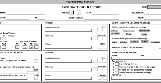
(21) Weber distinguishes the source of pure raw materials and the localized ones. The first, as they can be obtained at any point of, they are only affected by the weight of the final goods, so that reinforce attraction of the consumers center. The located raw materials, Webber separated them by pure and processable feedstock, for the last ones, they lose weight in the process productive, so they are reinforcing the attraction of sources of supply. The combination of all the elements determines the locational decision of each company. Taking the line of Weber`s work, the Swedish Palander (1935) attempted to develop a theory of spatial general equilibrium. Mainly he concentrated on studying the effects of prices on extensions market where companies can sell their products when the location, the competition conditions, the costs of factors and freight rates are given. Palander concluded that the benefits are based on the maximum distance that the company can expand its market. Hoover (1937) developed a model that is related to a spatial demand and marginal revenue, showing that there is an increasing price trend when transport unit costs grows, introducing the analysis of the spatial price discrimination. Now we see why there is in one point of production and on the other extreme we have a selling point or a market, and we need to use some sort of transportation to get from one point to another.. b. Objectives. . To elaborate a methodology to measure the CO2 emissions of the freight transport using a case study. We will use, with the kind authorization of the Department of Transportation of Tabasco, data from surveys made in Villahermosa - Tabasco in 2014 on the eastern corridor of México by the consulting firm LOGIT of Puebla.. . To analyze how different kinds of freight transport have a different effect on the production or emission of carbon particles into the environment.. . Finally, to look for different ways on how to improve the logistic of Mexico’s eastern corridor with the purpose of reducing CO2 emissions of freight transport in this country. 10.

(22) c. Instruments to use. In order to calculate the emissions of CO2 we need some variables. For this paper, we are using some variables taken from LOGIT surveys for the case of Villahermosa, Mexico; and for the rest of the cases are calculating the emission with the help of each case’s data. Required data: o. Origin-Destination o Distance traveled in kilometers. o. Truck model o Empty weight in kilograms.. o. Weight of the shipment to transport in kilograms. o. Empty travel or with a load.. o. Frequency of the travel (daily, weekly, monthly). Data to calculate: o. Average weight: statistic calculus of the average weight.. o. Distance of full travel.. o. Consumption of Diesel (C) liters of fuel, all the energy consumed for the shipment travel.. o. Kg of CO2 per liter of diesel used.. o. Kilograms of CO2 per all kilometers of full travel. o. Annual tons of CO2.. Statistical packages used: Stata is a general-purpose statistical analysis package created and maintained by StataCorp LP. Its capabilities include a broad range of statistical analyses, plus data management, graphics, simulations, and custom programming. Microsoft Excel is a spreadsheet developed by Microsoft for Microsoft Windows, Mac OS X, and iOS. It features calculation, graphing tools, pivot tables, and a macro programming language called Visual Basic for Applications.. 11.

(23) d. Methodology. Methodology to calculate the CO2 emissions of the freight transport There are many ways to calculate CO2 emissions in the atmosphere of the planet. For example in México, according to SEMARNAT (Secretaría de Medio Ambiente y Recursos Naturales) we use the following measures:. Table I.3 Methodologies to calculate CO2 in México •. Passive sampling: This method collects a specific contaminant through the adsorption. and/or absorption in a selected chemical substrate. After exposure by a suitable sampling period, which can vary from one hour to a few months or even one year, the sample returns to the laboratory where the desorption of the contaminant will be analyzed by its quantitative performance. The equipment used is known as passive samplers, presented in different shapes and sizes, mostly in form of tubes or discs. • Sampling Bioindicators: This method generally involves the use of living plant species, such as trees and plants, which serve as a receiving surface for contaminants. However, despite that scientists have developed guidelines on these methods, there are still unresolved issues in terms of standardization and harmonization of these techniques. • Active sampling: For this method we need power to suck the air to be sampled through a physical or chemical collection process. The additional volume of air sampled increases sensitivity, so we can obtain average daily measurements. The assets are classified as bubblers samplers (gas) and impactors (particles); among the latter, the most used currently is the high volume sampler "HighVol" . • Remote optical sensing method: The optical remote sensing method is based on spectroscopic techniques. Transmitting a light ray of a certain wavelength to the atmosphere and the absorbed energy is measured. With them it is possible to measure in real time, the concentration of various pollutants. Source: http://www.gob.mx/semarnat/documentos/inventario-de-emisiones. In table 1.2 it is possible to observe the different methods to calculate pollution in the atmosphere in Mexico, but we need to know something more specific such as the 12.

(24) pollution produced by freight transport. Therefore, by using some physics and chemistry laws we can find out the method used and developed by Professor Cristophe Rizet in Oct 2014, in his document “Quantification of freight Transport GHG emissions”. Now that we have the necessary or required variables for the calculation of CO2 emissions we will continue to perform the steps for calculating these emissions: i. - Step 1. Calculate the distances of transportation; this calculation was performed using the following equation: arc(AB) = 6371 * ArcCOS(COS(RADIANS(90-latB)) * COS(RADIANS(90-latA)) + SIN(RADIANS(90-latB)) * SIN(RADIANS(90-latA)) * COS(RADIANS(longDlongA))) Source: Christophe Rizet, Cécilia Cruz et Mathieu de Lapparent. (2014). Quantification des émissions de CO2 du transport de fret à partir de la base ECHO. En CO2-ECHO(1-29). MARNELA-VALLÉE. (PARIS-FRANCIA):. IFSTTAR.. However, technology helps us, making us our life easier, facilitating the calculation of the variable through the tool of Google: " Google Maps". 13.

(25) ii.- Step 2. Calculating the average load is a statistical calculation of the freight transportation, to take into our knowledge the round trip considering if it is full or empty, to have the statistical model, you can get the average load of the missing section of the journey replacing the data required in the following equation: Average load= 0.7087e0.1882*empty weight (truck with out cargo). Source: Own elaboration.. We can observe all the steps in the next diagram: iii. - Step 3. Calculation of liters of fuel consumed, in our case it will be done for all the vehicles which use Diesel. This consumption is calculated considering that there is a production of CO2 since the fossil fuel extraction, processing or refining to a useful fuel, transportation to distribution centers and finally to the vehicles to transport the products. The equation describing this consumption in liters is: Consume of Diesel liters per every 100 kilometers (C) = 3.5 x (Total Weight in kilograms + 4) 0.65 * Total weight in kilograms, is the weight of the empty vehicle plus the weight of the cargo or products. **In the case that we have an empty truck, we use the calculation of “Average weight” plus the weight of the empty truck, to calculate the total weight in kilograms.. 14.

(26) i.IV.- Step 4.- Calculation of C02 kilograms per liter of consumed Diesel. 1 liter of Diesel produces X number of kilograms of CO2 = 3.67 x 0.72 = 2.64 kg This equation means that of every liter of Diesel is 0.72 Kilograms of Carbon and when it combust in a motor of internal combustions, it produce 3.67 kilograms of CO2 and for every liter of Diesel used we obtain 2.64 kilograms of CO2.. V.- Step 5.- To calculate the CO2 tons emitted or produce on a route of freight transportation, we only calculate the next: Total distance X Liters of Diesel consumed X Kilograms of C02 per litter of Diesel 1000. and finally we obtain the total emitted tons of CO2 in a route of freight transportation.. VI. - Step 6.- And finally to obtain the total tones of CO2 in a year, we only made the. multiplication of the total tones of CO2 emitted in a route of freight transportation to the frequency of the journeys of this route in a year.. 15.

(27) Diagram I.1: Methodology to calculate CO2 emissions Total Tones of CO2. Calculation of total distance. Statistical Model. Google Maps. Average load calculation, according to the empty weight of the vehicle Source:. Consumption of Diesel (C) in liters of the total of energy used to transport the total of the cargo at highway: C = 3.5 x (Total Weight in kilograms + 4) 0.65 3.67 x 0.72 = 2.64 kg • 3. 1 L of Diesel emit 2.67 kg of Carbon and 1 Kg de Carbon generates 0.72 Kg of CO2. Christophe. Litters of Diesel consumed in every 100 Kms. Total distance X Liters of Diesel consumed X Kilograms of C02 per liter of Diesel 1000 X 20 or 40 Dollars per tone. Rizet, Cécilia Cruz et Mathieu de Lapparent. (2014). Quantification des émissions de CO2 du transport de fret à partir de la base ECHO. En CO2-ECHO(1-29). MARNE-LA-VALLÉE (PARISFRANCIA): IFSTTAR. 16.

(28) Chapter II: The best methods of logistics in the world (Road freight transport).. B.

(29) Road Freight Transport, Logistics and CO2 Emissions: Case study of Tabasco, Mexico Chapter II: The best methods of logistics in the world (Road freight transport). In this chapter we are going to describe the best methods of logistics in developed countries, but first we have to understand why the companies who are able to compete in domestic and international markets, face two big challenges; greater efficiency and lower costs, that’s why they are seeking access to the best supplies, no matter if they are in the domestic market or outside. They differentiate their products and services through the processes they use to deliver the goods to the final customers. Under the new conditions of high competitiveness, proper management of the supply chain and logistics play a very important role for companies, either for those who export or producing for the local market. The development of information technology has meant higher levels of productivity and less time and transaction costs, which has forced companies to rethink logistics management, to maintain and / or improve their competitiveness. Now, what is supply chain and logistics management? To understand better this concept we will describe what they are: The supply chain management: is the process for positioning and exchanging materials, services, semi-finished products, finished products, logistic of operations post- finishing, after-sales and reverse logistics, as well as information of integrated logistics, like procurement and procurement of raw materials, delivery and delivering finished products to the final consumer. The strategic planning of the supply chain, not only considers the final consumer, in other words, it doesn´t just consider the person or company who use a product or if the service is personal or a component to use to create other products, it also should consider intermediates, customers and it has to consider distributors and retailers. So it is important to know that the most important goals of the supply chain are: . Improve the productivity of operational logistic systems.. . Increase the services level for customers.. . Implement actions to get better management of operations. C.

(30) We just mentioned how to improve logistics administration with strategic planning of the supply chain, but what is logistic? For Jean-Paul Rodrigue in his third edition of the geographic transport system, logistic is: “It involves a wide set of activities dedicated to the transformation and distribution of goods, from raw material sourcing to final market distribution as well as the related information flows. Derived from Greek logistikos (to reason logically), the word is polysemic. In the Nineteenth century the military referred to it as the art of combining all means of transport, revictualling and sheltering of troops. In a contemporary setting, it refers to the set of operations required for goods to be made available on markets or to specific locations.” In simple worlds, logistic is the link between the market and the operational activity of the company; it covers the entire organization, from management of raw materials to finished product delivery. This involves the management of information flow, cash and product-service. The principal activities of logistics are classified in two:. Level of client services Order processing Key activities. Inventory management Transport. Storage Goods handling Support activities. Packing Purchases Information management Information processing. In the present time, the trend for companies is to contract specialized logistics operators for tasks like: inventory management, warehousing and distribution, in an integrated manner. The main contribution of the outsourcing is that when they perform this task for several companies, simultaneously; they achieve significant improvements on the economies in the above activities (warehouse management, inventory management and 18.

(31) consolidation in transportation). Outsourcing services can be an alternative to improve the competitiveness of enterprises. This practice provides benefits that allows them to focus the companies energy to its reason for being (whatever they produce), leaving aside all those activities for which they are not specialists. Some reasons that outsource logistics services are important: . Concentrate in base activities.. . Invest fewer resources in support activities.. . Facilitate access to technology and equipment for moving freight, warehousing and information systems.. . Low operating cost by the logistics operator.. . Access to a better understanding of the distribution of goods. . Access to qualified and specialized human resources.. . Reduce or control spending of operations.. There are a lot of topics to analyse and study but for the interest of this investigation what is important is the logistic of freight transport. To understand better the freight transport we are going to study the best examples of it, in Europe we can find some of the best examples of freight transport, without frontiers to stop every time they cross a country, they have one of the best freight transport examples. a. Europe. (EU) As we mentioned before, Europe is one of the best examples of freight transport, as the European Commission of Mobility and Transport let us know that the principal objective of the European Union’s land transport policy is promote a mobility that is efficient, safe, secure and environmentally friendly, also create fair conditions for competition to promote safer and more environmentally friendly technical standards, to guarantee that road transport rules are applied effectively and without discrimination. According to the “Road Transport, A change of gear” of the European commission we can know that the road transport is the most important of the freight transports in de European Union, with 45.9% of the total of the goods transport in 2010, we can find it and the rest of the transport in the next graphic:. 19.

(32) Graphic II.1: Distribution of the freight transportation in EU, 2010. Source: Road Transport a change of gear report, 2010. For the European Union, the internal market of freight transportation by road has been open since December 2011; the EU has been establishing a set of rules to ensure fair competition between road transport operators. The open internal market created the possibility for transport companies to supply services across national borders. To do it, they must respect all the common regulations, for transportation of goods or passengers between countries members of EU. All the National authorities are carrying out regular checks to ensure that transport companies are attempting the next four criteria: Table II.1: Criteria for the road transport companies, 2011. 1. 2. 3. 4. Good repute: professional operators must meet adequate ethical and entrepreneurial standards. Failure to apply or respect EU rules will mean exclusion. Sound financial standing: each year, operators need to show capital assets equivalent to €9 000 for the first vehicle and €5 000 for each additional vehicle. Professional competence: operators must pass a standard exam to assess their practical knowledge and aptitude. Establishment: operators must demonstrate that they have an effective and stable establishment in an EU Member State. Source: Road Transport a change of gear report, 2010. 20.

(33) Also for operation, all companies need to have a permission or license to have their vehicles or operate them in the European Union; they call it community license from their own Member State, which allows them to carry out cross-borders transport through al the European Union. They have to carry certified copy of the community license in every of their vehicles. Drivers from non-EU countries must carry a certificate, which proves that they are legally employed by a licensed EU road operator. They standardized the type of vehicles for freight transport; they set limits for weight and dimensions for heavy-duty vehicles in Europe, and this is to prevent damage of the roads bridges and any kind of infrastructure, and principally to ensure safety on the roads, at the next table we are going to find the permit weight the cargo in freight transport: Heavy goods vehicles come in different sizes: . Starting with small vehicles with load capacity from 3.5 tons to a maximum permissible of 6 tons. . Smaller heavy goods vehicles are those with a maximum weight of up to 20 tons. . Big vehicles are those with a maximum weight is between 20 to 40 tons or 44 tons when the vehicle is carrying a container for combined transport operations. Sizes:. Classification of freight transport vehicles.. In the European Union they are trying to improve their logistics and then decrease their empty vehicle travels, for that they are using the method of Cabotage. It is one way to reduce congestion and increase their freight transport efficiency. Cabotage allows all drivers from one country to transport goods to another country on a temporary basis when they are making international deliveries. In other words, if the truck has to deliver in some places, lets say Paris, and it is from a Brussels truck and it has to drive empty to 21.

(34) pick up a return load in Strasbourg, it can carry goods from Paris to Strasbourg. Operators from all the Member States are free to carry out temporary cabotage cargo. Graphic II.2: EU road freight transport by type of operation in 2010. Source: Road Transport a change of gear report, 2010. Another way to improve the logistics in Europe, is using some technology like an interoperable electronic tolling service; this technology is a compatible national electronic tolls systems and it is a legal requirement since 2007; it helps to reduce delays and congestion. The EU legislation provides an European electronic toll service (EETS), that’s why road users can subscribe to a single contract with one service provider, and using a single on-board unit to pay tolls electronically through all the EU. The elimination of cash transactions at tollbooths, traffic flows would be improved and congestion will decrease. Technology can help to improve an efficient use of infrastructures, transport management and a smaller carbon footprint. Also smart logistics can help to reduce the number of empty journeys made by trucks, which still account for nearly 25% of the total, according to the European Commission of mobility and transport. Galileo, the European satellite navigation system, and other navigational technologies are also helping to reduce journey times, provide real-time information to reduce congestion and offer track-and-trace monitoring for vehicles and cargos, also helping preventing cargo theft and rapid assistance to motorists involved in a collision and then they are increasing road safety, real-time traffic and multimodal travel information services. We just analysed what is happening in the European Union; in this continent we can find out that the performance of the logistics is really good, according to de World Bank and its Logistics Performance Index (LPI) we know that the index of Europe is 3.32 units, 22.

(35) where 1 is low (Bad logistics) and 5 is high (Good logistics), this index is based “on a worldwide survey of operators on the ground (global freight forwarders and express carriers), providing feedback on the logistics “friendliness” of the countries in which they operate and those with which they trade. In this index, they combine knowledge of the countries in which they operate with informed qualitative tasks of other countries where they trade and experience global logistics environment. Feedback from operators is supplemented with quantitative data on the performance of key components of the logistics chain in the country of work. The LPI consists of qualitative and quantitative measures and helps build profiles of logistics friendliness for these countries. It measures performance along the logistics supply chain within a country (World Bank, 2016). According to LPI, we observe that one of the highest performances is Germany with 4.12, then Belgium with 4.04, United States of America with 3.92, France with. 3.85 units (this country grew from 3.76 units in 2007, so they are improving all the time to have better logistics on their transport). Now we can observe how the freight transport in France is in the last years: Table II.2: Distribution of modal of land freight transport (% of TonsKilometres 2004. 2005. 2006. 2007. 2008. Transport ferroviaire. 11.9. 10.6. 10.3. 10.3. 10.2. 9.3. 8.4. 9.5. 9.5. 9.3. 9.5. Transport routier. 80.9. 81.9. 82.2. 82.7. 82.6. 82.8. 84.4. 83.6. 83.9. 85.0. 85.0. 1.9. 2.0. 2.0. 1.8. 1.9. 2.2. 2.3. 2.2. 2.3. 2.3. 2.3. Navigation fluviale oléoducs Tous modes (Gt-km). 2009. 2010. 2011. 2012. 2013. 2014. 5.3. 5.4. 5.6. 5.1. 5.3. 5.7. 4.9. 4.8. 4.4. 3.4. 3.3. 389.5. 384.5. 399.9. 412.4. 396.5. 343.7. 356.8. 361.3. 343.9. 343.5. 339.6. Sources: SOeS d'après Eurostat, DGEC, VNF. With this table it is easy to note that freight transport by truck is more common than the other types. b. America In America we have two countries with great logistics, United States of America and Canada, with a LPI of 3.92 and 3.76 respectively, in USA the industry of logistics and transportation is highly competitive. In the United States, they are investing in this sector; multinational firms position themselves to improve the flow of goods through all the world market, international and domestic companies benefit from a highly skilled workforce, low costs and cargos regulation. USA spends in logistics and transportation a total of $1.45 trillion in 2014, and it 23.

(36) represents 8.3 percent of annual gross domestic product (GDP). They have supply chain network links producers and consumers through multiple transportation modes, including air, freight rail, maritime transport, and truck transport, this last one is of our interest. Over the road cargo transportation is provided by motor vehicles over short and medium distances. In USA, the trucking associations report that their vehicles move 9.2 billion tons of cargo and is the predominant modal of all cargo domestically transported. According to the U.S. department of transportation, the Federal commercial vehicle maximum standards on the Interstate Highway System are: Single Axle:. 9070.84 Kilograms. Tandem Axle:. 15420.428 Kilograms. Gross Vehicle Weight:. 36283.36 Kilograms. Table II.3.Federal Commercial Vehicle Size Limits on the National Network No federal length limit is imposed on most truck tractor-semitrailers operation on Overall the National Network. vehicle Exception: On the National Network, combination vehicles (truck tractor plus length semitrailer or trailer) designed and used specifically to carry automobiles or boats in specially designed racks may not exceed a maximum overall vehicle length of 19.82 meters, or 22.86 meters, depending on the type of connection between the tractor and trailer. Federal law provides that no state may impose a length limitation of less than Trailer 14.63 meters (or longer if provided for by grandfather rights) on a semitrailer length operating in any truck tractor-semitrailer combination on the National Network. (Note: A state may permit longer trailers to operate on its National Network highways.) Similarly, federal law provides that no state may impose a length limitation of less than 8.5344 meters on a semitrailer or trailer operating in a truck tractorsemitrailer-trailer (twin-trailer) combination on the National Network. On the National Network, no state may impose a width limitation of more or less Vehicle than 2.5908 meters. Safety devices (e.g., mirrors, handholds) necessary for the safe width and efficient operation of motor vehicles may not be included in the calculation of width. No federal vehicle height limit is imposed. State standards range from 4.15 meters Vehicle to 4.45 meters. height Source: U.S. Department of Transportation, Federal Highway Administration. Federal Size Regulations for Commercial Motor Vehicles. (Washington, DC: 1996).. Like in Europe, USA uses a multimodal model for their freight transportation; having seen how they have their regulation for vehicles of road transport, we can understand 24.

(37) why it is so important to study this kind of transport and why they are making so much efforts to improve it, in the next table we can find how the freight transport by truck is more used than the others, with 40.24% of the total, according to the estimates of the Bureau of Transportations Statistics the distribution of the freight transport is: Table II.4.; Distribution of the freight transport in USA, 2011. Mode of Freight Shipments Truck Rail Water Air & Air/Truck Pipeline Multiple modes Other & Unknown Total. 2011 Ton miles (in billions) 3761.03 2442.98 698.45 17.70 1638.31 786.97 149.67 9345.44. Percent of Total 40.24% 26.13% 7.47% 0.19% 17.53% 8.43% 1.60% 100%. Source: Estimates by the Bureau of Transportation Statistics, 2011. One of the principal characteristics of the freight transport in USA, is that they know that the majority of their merchandises is transported by truck, they are trying to improve not only their logistics at the road, they are also doing it at their warehouses, developing new techniques for the logistics but the most important idea is that they are getting better use of the solar energy, using it to energize warehouses and helping the environment, accelerating their processes of logistics using some technology to improve and automatize the processes. Solar system are used by FedEx in Woodbridge, N.J.. The solar power project is the third between a FedEx operating company and BP Solar and the fifth solar power project for FedEx. The 2.42-megawatt solar power system covers approximately 3.3 acres of roof top space with approximately 12,400 solar panels. Another case to study in America is Canada, with a LPI of 3.86; they have 1.3 million two-line of roads, this case is interesting because is a really large country and it is not so populated, with 35 749 600 habitants and 9 984 670 km² of surface, Canada has a great logistics so it is remarkable to mention it. In December 2014, there were 62,805 businesses whose primary activity was trucking transportation. It includes many small for-hire carriers and owner-operators, and some medium and large for-hire companies that operate fleets of trucks and offer logistic services. The trucking industry can be divided into three main types of trucking activities: 25.

(38) . For-hire trucking services is to classifications: Less-than truckload (LTL), and Truckload (TL) and for-hire carriers can be further grouped as: Intra-provincial (operating exclusively within a provincial jurisdiction) and Extra-provincial (beyond provincial and national boundaries).. . Courier operators, who specialize in transporting parcels.. . Private carriers, where businesses maintain a fleet of trucks and trailers to carry their own goods. These carriers’ activities are not tracked, as they are part of companies whose main line of activity is not trucking for example Wal-Mart, Costco.. Their regulations according to The Federal-Provincial-Territorial Memorandum of Understanding on Interprovincial Weights and Dimensions are: Table II.4. Heavy Truck Weight and Dimension Limits for Interprovincial Operations in Canada Classification. Its length, including load, does not exceed:. Its Gross Combination Weight does not exceed:. Category 1: Tractor Semitrailer Category 1A: Tridem Drive Tractor Semitrailer Category 2: A Train Double Category 3: B Train Double. 23 metres 23.5 metres. 46 500 kg 52 300 kg. 25 metres 27.5 metres. 53 500 kg 62 500 kg. Category 4: C Train Double Category 5: Straight Truck Category 6: Truck - Pony Trailer Category 7: Truck - Full Trailer Category 8: Intercity Bus and Recreational Vehicles. 25 metres 12.5 metres 23 metres 23 metres 14 metres. 58 500 kg 24 250 kg 45 250 kg 53 500 kg 24 250 kg. Source: The Federal-Provincial-Territorial Interprovincial Weights and Dimensions, 2014. Memorandum. of. Understanding. on. We know their regulations but with long distances to drive, why are they so safe and have a great logistics? An answer this question is that since 2014, the Government of Canada amended the Motor Vehicle Safety Act to further strengthen Canada’s vehicle safety regime. These amendments included doubling criminal financial penalties and giving the 26.

(39) Minister of Transport the authority to order vehicle manufacturers to issue notices of defect or non-compliance. This helped to ensure Canadians are informed of any safety or non-compliance issues with their vehicles. In 2013, Canada upgraded the Motor Vehicle Tire Safety Regulations with stricter tire safety standards, aligning its tire safety regulations with the U.S. to create and reduce costs for manufacturers and consumers, this is according to the Overview report of transportation in Canada by the minister of transport, 2015. At the beginning of this chapter we described what is the supply chain and logistics, now we have seen that freight transport is an important part of the logistic of the supply chain, industry needs to transport goods from one place to other and to do it as we showed during this chapter they use freight transport by truck, with the analysis of the last cases we know that the freight transport by truck is the most used and important type of transportation in the developed countries of the world economy.. 27.

(40) Chapter III: Logistics, road freight transport in México and its problems.. C.

(41) Road Freight Transport, Logistics and CO2 Emissions: Case study of Tabasco, Mexico. Chapter III: Logistics, road freight transport in México and its problems.. In the first quarter of 2016, Mexico grew at an annual rate of 2.6 % according to the first revision of GDP of INEGI (National Institute of geographic statistics information), also in the last 5 years México increased the exportations of its manufacturing by 6.2% according to the same institute, because of the world slow economy México is experimenting a decrease of its exportations by 1.7 % in the last months. Table III.1. Total exportations and importations by classification of transport, 2006 and 2015. 2006 Millions of Dollars (USA) Exportations Importations. 8,693 20,954. Exportations Importations. 59,544 55,269. Exportations Importations. 153,736 139,415. Exportations Importations. 25,254 15,350. Exportations Importations. 2,770 25,142. % Of Total By Air 3.5% 8.29% By Water 23.8% 21.6% By road 61.5% 54.49% By train 10.1% 6.0% Others 1.1% 9.8%. 2015 Millions of Dollars (USA). % Of total. 8,663.6 4.4% 16,8893.5 9.4% 35,123.2 19% 59,178.2 31.1% 117,302.2 62.2% 97,687.8 50% 26,978.8 14.1% 16,144.4 8% 520.3 0.3% 2686.2 1.5%. Source: Own elaboration with data of INEGI 2015. With the last table we see that the trade of products has been decreasing by water transportation in the last years, exclusively the exportations, and increasing the transportation by air, train and road. Mexico is also receiving a lot of companies to produce in its territory, principally Transport manufacturing companies, for example; KIA, BMW, AUDI and others, with 28.

(42) more manufacturing production in the Mexican territory, it is necessary to have a great logistics of freight transport by truck.. a. Logistics of road freight transportation in México. According to the Mexican Institute for Competitiveness (IMCO), Mexico is ranked 61th of 144 countries in the Global competitiveness index, 2014-2015, this is bad for our country, the position of Mexico in 2013-2014 was the 55, which means that we retreated 5 positions in one year. The LPI of Mexico is 3.13 with this index we can figure how far México is from the best logistics of developed countries, this indicator let us analyze the next points: . Level of efficiency in the process of customs clearance by border agencies.. . Quality of transport infrastructure and information technology in the logistics field.. . Practice of foreign trade in terms of cost and feasibility transport.. . National Competition in the logistics sector.. . Ability to trace and track international shipments.. . Domestic logistics costs, transport category.. . Times of destination.. Table 3.2. LPI per study area in México. Frontiers (Customs) Infrastructure International shipments Logistic competence Pacification and following of goods delivery Logistic Costs Times. Place/144 countries 60 53 53 57 48 101 51. Points/(1 min, 5 max) 2,5 2,68 2,91 2,8 2,96 2,79 3,4. Source: Own elaboration with World Bank data.. Also the analysis of AT Kearney in their article “Agenda de competitividad en logistica 2008-2012” shows that Mexican freight transport has 88 percent of cases with on-time deliveries of goods; against 97 in the US and 98 percent in European countries. In other point, safety in freight transportation, Mexico only has 89 percent of cases that 29.

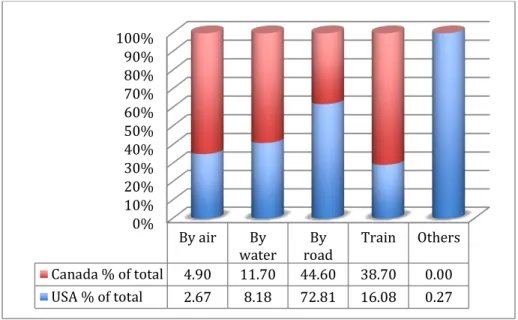
(43) complete their destination, while in the United States and Europe the average is 97 percent. Mexico as many other countries in Latin America, the road network is the most important and used transport infrastructure, the national road network, communicates almost all regions and cities. Mexico has 378,923 km of roads, for highways, federal roads, rural roads and others that allow connectivity between almost all populations in the country, in other worlds, there is a connection for people that has economic relevance, to every place. Our principal destination is USA and Canada, because of the North American Free Trade Agreement (NAFTA), so we have to know how do we import and export our products from those countries, at the next graphics we will analyze the traffic by the type of transport that we use to trade products. Graphic III.1. Exportations of NAFTA by classification of freight transport (% percent of the total) 100% 90% 80% 70% 60% 50% 40% 30% 20% 10% 0%. By air. Canada % of total. 4.90. By water 11.70. USA % of total. 2.67. 8.18. By road 44.60. Train. Others. 38.70. 0.00. 72.81. 16.08. 0.27. Source: Own elaboration with data of INEGI 2015. 30.

(44) Graphic III.2. Importations of NAFTA by classification of freight transport (% percent of the total) 100% 90% 80% 70% 60% 50% 40% 30% 20% 10% 0%. By air. Canada % of total. 7.69. By water 15.32. USA % of total. 3.64. 11.21. By road 57.30. Train. Others. 19.54. 0.15. 66.88. 15.10. 3.17. Source: Own elaboration with data of INEGI 2015. According to the graphics 3.1. And 3.2. We can find out that the exportations and importations of products to those countries are mostly by truck or road freight transportation, the second type of transportation is by train and closely to this one is by shipments or water. Mexico to get better logistics and improve the supply chain to those countries has to study and analyse what is doing good and wrong, this is because we already know that the logistic of México is not to good, as we mention earlier the LPI of México is not really high so we know that is necessary to improve it. We have to know what are the regulations of the road freight transport in México and the characteristics of the infrastructure for the road freight transport. We already know how long are the roads of México, and they connect almost every place in México but we have to know how much they cost for the freight transport, according to the graphics 3.3. We can observe that for small distances they cost more than when there is a long distance, with a cost of 3.75 Dollars per kilometer of the first 50 kilometers, but long distances, lets say a distance of 800 kilometers, every kilometer costs 0.6 dollar.. 31.

(45) Graphic III.3. Curve of road transport cost, (Inside the countries, kms-Dollars). Source: Own elaboration with of Database A.T. Kearney, Displays over 10,000 points.. We have seen that every kilometer has different costs according to the distance to travel, our next step is to know which are the most used corridors in México, according to the Secretary of communications and transport of Mexico (SCT), at the table 3.3. We can note that the most used corridors are those which go out from the principal states of México, like Mexico, Jalisco, Nuevo Leon, but the most important of them are the corridors which involves México city, from this city goes most of the travels to any place to the country.. 32.

(46) Table III.3. Principal corridors of road freight transport, 2014 (Average of tons per day) Corridors Baja California - Baja California Sonora - Sonora Chihuahua - Chihuahua Tabasco - Tabasco Veracruz - Tabasco Sonora - Baja California Distrito Federal - Baja California Sonora - Chihuahua Distrito Federal - Tabasco Sonora - Sinaloa Tabasco - Campeche Yucatan - Tabasco Distrito Federal - Yucatan Jalisco - Baja California Nuevo Leon - Chihuahua Nuevo Leon - Baja California Coahuila - Chihuahua Sonora - Nuevo Leon Chihuahua - Baja California Tabasco - Chiapas Sinaloa - Baja California Distrito Federal - Sonora Yucatan - Veracruz Quintana Roo - Veracruz. Daily Average Tons Go Back Total 33,261 33,261 15,796 15,796 15,745 15,745 12,410 12,410 4,897 4,361 9,258 3,562 2,528 6,090 3,56 1,591 1,591 2,099 1,923 4,022 2,191 1,055 3,246 1,973 1,110 3,083 1,664 755 2,419 1,075 1,062 2,137 901 821 1,722 1,098 612 1,710 1,234 333 1,567 855 633 1,488 871 575 1,446 853 534 1,387 852 472 1,324 574 525 1,099 685 354 1,039 647 505 782. 354 423. 1,001 928 782. Corridors Jalisco - Sonora Tabasco - Quintana Roo Veracruz - Campeche Tabasco - Puebla Distrito Federal - Quintana Roo Distrito Federal - Chihuahua Baja California Sur - Baja California Durango - Chihuahua Distrito Federal - Campeche Baja California - Mexico Mexico - Yucatan Chihuahua - Sinaloa Puebla - Yucatan Nuevo Leon - Tabasco Jalisco - Chihuahua Jalisco - Yucatan Queretaro - Baja California Chihuahua - San Luis Potosi Yucatan - Chiapas Yucatan - Nuevo Leon San Luis Potosi - Sonora. Daily Average Tons Go Back Total 502 274 776 523 191 714 621 76 697 340 304 644 464 161 625 345 279 624 317 238 555 304 187 491 197 161 358 344 344 275 275 168 91 259 189 69 258 207 51 258 236 236 217 217 203 203 109 71 180 168 168 161 161 52 36 88. Mexico - Chihuahua Coahuila - Sonora. 78 44. Source: Own elaboration with data of Technical document No. 48 "Estudio Estadístico de Campo del Autotransporte Nacional".. 33. 78 44 0.

(47) SCT has some control of the registration of vehicles; they approximately counted 576200 vehicles in total for road freight transport, they classified them for the type of company in the country. Graphic III.4. Classification of vehicles and percentages of the total of vehicles in Mexico, 2010. 576,200 Vehicles (Total trucks) Bigh companies. 14% 49%. 16%. 21%. Medium companies Small companies Man truck (hombre camion). Source: Own elaboration with data of SCT, 2011. **Man truck: person who owns a vehicle and rent his or her services to companies for freight transport or who ever pays them for the travel.. In the last graphic we can find out that Mexico has a lot of Man truck, and it is a big problem, they don´t have coordination with the companies and the supply chain so they don´t have good logistics. With this notification we can understand why the age of the vehicles in Mexico is a little critical, according to the SCT the average age of the vehicles is 15.5 years old. The maximum sizes and weights are important to know, because with them we can analyze better the behaviour of the freight transport in México. In the next tables we describe the types of vehicles in Mexico:. 34.

(48) Table III.4.a Classification, Maximum length and weights of road freight transport vehicles (México, 2014) Vehicular Number Number GVWR Dimensions classification of axes of (tons) Large Width Height Figure wheels (m) (m) (m) C2 2 6 19,0 23 2.6 4.25 C3. 3. 8. 24,0. 23. 2.6. 4.25. C3. 3. 10. 27,5. 23. 2.6. 4.25. C2-R2. 4. 14. 37,5. 31. 2.6. 4.25. C3-R2. 5. 18. 44,5. 31. 2.6. 4.25. C3-R3. 6. 22. 51,5. 31. 2.6. 4.25. C2-R3. 5. 18. 44,5. 31. 2.6. 4.25. T2-S1. 3. 10. 30,0. 23. 2.6. 4.25. T2-S2. 4. 14. 38,0. 23. 2.6. 4.25. Source: Own elaboration with statistics of SCT.. 35.

(49) Table III.4.b Classification, Maximum length and weights of road freight transport vehicles (México, 2014) Vehicular Number Number GVWR Dimensions classification of axes of (tons) Large Width Height Figure wheels (m) (m) (m) T3-S2 5 18 46,5 23 2.6 4.25 T3-S3. 6. 22. 54,0. 23. 2.6. 4.25. T2-S3. 5. 18. 45,5. 23. 2.6. 4.25. T3-S1. 4. 14. 38,5. 23. 2.6. 4.25. T2-S1-R2. 5. 18. 47,5. 31. 2.6. 4.25. T2-S1-R3. 6. 22. 54,5. 31. 2.6. 4.25. T2-S2-R2. 6. 22. 54,5. 31. 2.6. 4.25. T3-S1-R2. 6. 22. 54,5. 31. 2.6. 4.25. T3-S1-R3. 7. 26. 60,5. 31. 2.6. 4.25. Source: Own elaboration with statistics of SCT.. 36.

(50) Table III.4.c Classification, Maximum length and weights of road freight transport vehicles (México, 2014) Vehicular Number classification of axes T3-S2-R2. 7. Number of wheels 26. GVWR (tons). Dimensions. T3-S2-R4. 9. 34. 66,5. 31. 2.6. 4.25. T3-S2-R3. 8. 30. 63,0. 31. 2.6. 4.25. T3-S3-S2. 8. 30. 60,0. 31. 2.6. 4.25. T2-S2-S2. 6. 22. 51,5. 31. 2.6. 4.25. T3-S2-S2. 7. 26. 58,5. 31. 2.6. 4.25. 60,5. Large (m) 31. Width (m) 2.6. Height (m) 4.25. Figure. Source: Own elaboration with statistics of SCT.. 37.

(51) With the last table we see that there are many classifications in México for the vehicles of road freight transport, not because they are so different, it is because of the number of axes and wheels at the axes, those two things help for the stability, tractions and cargo distribution, of the vehicles of road freight transport. The lengths, hights and widths are similar, the only variable which changes is the first one, and it is because of the extra cargo.. b. Common problems of freight transportation in México. Mexico has a lot of problems with the freight transportation by truck; some of them are caused by bad coordination of the companies of freight transport with the industry, or just between transport companies drivers and warehouses. In this country one of the biggest problems is the classification of freight transport named man truck, according to the graphic 3.4 they are more vehicles like that than the vehicles of transport companies. For man truck it is easy to just drive and provide their services for some amount, the problem is that they don´t have the technology and organization to comply correctly the times and specifications of a contract, and the penalties are low for this kind of transport. Next, here are the most common problems in Mexico: . The cost of the travel does not depend every time on the distance and the weight of the cargo, in Mexico the problem is that the price depends on the zone, if it is problematic or dangerous it costs a lot more than in other zone, and of course the insurance of the cargo costs more.. . Highways are expensive, unsafe and in bad condition, most of the time.. . Often the road freight transportation companies don´t have the right equipment for the transportation of the cargo, most of the time they have bigger dimensions and that increases the price of the travel.. . The warehouses have not the right size for all the cargo of an average day, and sometimes the receiving company doesn’t even has a warehouse, so the vehicle has to wait a long time parking outside and the companies have to pay extra time.. . Vehicles are old and they break down in the middle of the travel.. . Companies pay to use the toll highways but drivers use the free roads. 38.

(52) . Bad logistics to unload the cargo of the truck, if the drivers travels at night, whey they arrive to the destination they just park and sleep and then they unload the cargo until noon.. In conclusion, Mexico must think about the logistics of the freight transportation, because with a simple analysis we can find that there are a lot of problems with the organization of logistics, the technology of the vehicles and null technology and organization for a safe travel of the driver and the cargo to arrive at destination.. 39.

(53) Chapter IV: Method to calculate carbon emissions. D.

(54) Road Freight Transport, Logistics and CO2 Emissions: Case study of Tabasco, Mexico 4. - Chapter IV: Method to calculate carbon emissions. As seen in chapter 1, in México we have various methods to calculate the production or the emission of CO2 in the country. In this chapter we are going to analyze the most common variables for the calculation of CO2 emissions of the freight transport in México in the Tabasco corridor. In this particular case we can observe different logistic routes and search how the freight transport from different origins and destinations have typical or untypical behaviour. d) Variables to use to calculate carbon emissions. First, we have to know which variables we are able to work with. Required data: o. Origin-Destination o Distance traveled in kilometers.. o. Model of truck. o Empty weight in kilograms.. o. Weight of the shipment to transport in kilograms.. o. Empty travel or with products.. o. Frequency of the travel (Daily, weekly, monthly).. Data to calculate: o. Average weight: statistic calculus of the average weight.. o. Distance of full travel.. o. Diesel consumption (C) litters of fuel, all the energy consumed of the shipment travel.. o. Kg of CO2 per litter of Diesel used.. o. Kilograms of CO2 per total kilometers of full travel.. o. Annual tons of CO2.. With the data of the case of Tabasco we have to prepare the variables for the calculation of CO2 emissions of the freight transport. 40.

(55) Diagram IV.1. Methodology of the variables To order my variables Find out which variable is useful and erase those whose are not Step 1: Order by final destination A: By State B: Every State by City Step 2: Order by origin. Using the last classification of step 1. A: Order by State B: Every State order by City. Step 3: Search in Google Maps the distance of the road. Step 4: Calculate the weight of the cargo. A: Order the variables by type of cargo. B: Use the classification of units of cargo. Table IV.1.1. Classification and weight of the cargo. Source: Own elaboration with data of LOGIT case of Tabasco C: Convert everything in kilograms. Step 5: Calculate frequency A: Order all data by kind of frequency. B: Calculate total frequency: Total= Frequency of the road X Frequency of the period X Frequency of the year Step 6: Create binary variable “Empty” A: Order by empty or not B: Empty: 0 = Not empty 1= Empty. 41.

(56) Step 7: Weight of the empty transport. A: Find out the model of the transport vehicle. B: Use the table of classification of vehicle weights.. Table IV.1.2. Classification and weight of the cargo. Source: Own elaboration with data of LOGIT case of Tabasco 42.