Escuela de Ingeniería en Computación
Programa de Maestría en Computación
Application of Nearest Neighbour
Search techniques to Peptide
identification from Mass Spectrometry
A thesis submitted in partial fulfilment to opt for the degree of
Magister Scientiæ
in Computer Science
Author
José de Jesús Ulate Cárdenas
Supervisor
Francisco Torres Rojas, PhD.
To my beloved Julia and Antonio, my grandparents. For all the years of joy that I will never forget.
Acknowledgements
I want to thank Alejandro Fernández Woodbridge, PhD, researcher of the Science for Life Laboratory in Stockholm, Sweeden; who provided the initial inspiration for this research. Luis Alejandro Acuña Prado, MSc, mathematics professor of the Costa Rica Institute of Technology, whose course of Functional Analysis and Topology gives us the necessary formality and support. Bruno Lomonte, PhD, researcher of the Clodomiro Picado Institute, who guided us and provided profound insights and revisions of the research results.
Nancy Peréz, MSc, Statistics analyst of the Costa Rica Central Bank, and Ivania Montero, Oficial Translator of the Ministry of Foreign Affairs and Worship of Costa Rica, for the English corrections of this document.
National Collaborative of Advanced Computing (CNCA) of the Costa Rica National High Technology Center (CENAT) for providing the infrastructure for execution of many tests.
Abstract
We explored if the application of Nearest Neighbour Search thecniques to thede novo
Resumen
Exploramos si la aplicación de las técnicas de búsqueda del vecino más cercano a la identificación de novo desde Tandem Mass Spectrometry proveería un mejor
Contents
1. Introduction 1
1.1. Problem . . . 3
1.2. Document Structure . . . 4
2. Theoretical Framework 7 2.1. Molecular Biology . . . 8
2.1.1. Amino Acids . . . 8
2.1.2. Proteins . . . 14
2.1.3. Peptides . . . 14
2.1.4. Post-Translational Modification . . . 14
2.1.5. Proteogenomics . . . 18
2.1.6. Mass Spectrometry . . . 20
2.1.6.1. Mass Spectrometry Technique . . . 20
2.1.7. High-resolution Isoelectric Focusing Liquid Chromatography Mass Spectrometry . . . 22
2.1.8.1. Peptide Fragmentation . . . 24
2.1.8.2. Definition . . . 29
2.1.8.3. Spectrum Graphs . . . 29
2.1.8.4. Peptide Sequence Problem . . . 31
2.2. Mathematical Fundamentals . . . 37
2.2.1. Set Theory . . . 37
2.2.2. Algebraic Structures . . . 40
2.2.3. Topology. . . 46
2.3. Computer Science . . . 52
2.3.1. Nearest Neighbour Search . . . 52
2.3.1.1. Space Partitioning . . . 52
2.3.1.2. R-Tree . . . 52
2.3.2. Locality Sensitive Hashing . . . 54
2.3.2.1. Jaccard Similarity of Sets . . . 54
2.3.2.2. Min Hash . . . 54
2.4. Related Work . . . 56
2.4.1. MS-GF+. . . 56
2.4.2. Mascot . . . 57
2.4.3. HiXCorr . . . 58
2.4.4. Sailfish . . . 58
2.4.5. SEQUEST . . . 59
2.4.6. Tempest . . . 60
2.4.7. OpenMS . . . 60
2.4.8. PepNovo . . . 61
2.4.9. Other Investigations . . . 61
3.1.1. Main Objective . . . 64
3.1.2. Specific Objectives . . . 65
3.1.2.1. Index Creation . . . 65
3.1.2.2. Search Engine Creation . . . 65
3.1.2.3. Evaluation of the Metrics . . . 65
3.2. Proposed Approach . . . 65
3.2.1. Analysis of Variance . . . 66
3.2.2. Results Analysis . . . 66
3.2.2.1. Alternative and Null Hypotheses . . . 67
3.2.3. Original Metrics. . . 67
3.2.3.1. FDR Metric . . . 67
3.2.3.2. COV Metric. . . 67
3.2.3.3. ET Metric. . . 67
3.2.4. Original Hypothesis. . . 68
4. Results and discussion 69 4.1. De novo Approach . . . 70
4.1.1. Notation and Definitions . . . 71
4.1.2. Indexation . . . 75
4.1.3. Search Algorithm . . . 78
4.2. Deliverable List . . . 87
4.2.1. Source Code . . . 87
4.2.1.1. Indexation Prototype. . . 87
4.2.1.2. Search Engine Prototype. . . 87
4.2.2. Mathematical . . . 87
4.2.2.1. Analysis of Metrics . . . 87
4.3. Indexation . . . 88
4.4.1. Metrics review. . . 94
4.4.1.1. AMB Metric . . . 94
4.4.1.2. COV Metric. . . 94
4.4.1.3. ET Metric . . . 95
4.4.2. Error at High Resolution . . . 95
5. Conclusions, recommendations, and future work 97 5.1. Conclusions and Recommendations . . . 98
5.1.0.1. Understanding the “Shape” of the Problem . . . 99
5.2. Future Work. . . 100
5.2.1. Extension of the Model . . . 100
5.2.1.1. Extension of the Amino Acid Alphabet . . . 100
5.2.1.2. Results Refinement . . . 100
5.2.1.3. Other Ion Types Detection . . . 100
5.2.1.4. Consideration of Fragmentation Methods . . . 101
5.2.2. Optimisation . . . 101
5.2.2.1. Reduction of Index Building Time . . . 101
5.2.2.2. Reduction of Search Running Time . . . 101
5.2.3. Variable Behaviour . . . 101
5.2.3.1. Study of how an Admissible Error affects Running Time and Ambiguity . . . 102
5.2.4. Large-Scale and Complex Data Sets and Evaluation . . . 102
5.2.4.1. Database Assisted Interpretation . . . 102
5.2.4.2. Solution Discrimination . . . 102
5.2.4.3. Performance and Accuracy Analysis with more de novo Software Packages . . . 102
6.1. Index Prototype Source Code . . . 106
6.1.1. Index generation header . . . 107
6.1.1.1. Memoization speed up . . . 107
6.1.1.2. Program arguments . . . 107
6.1.1.3. Implementation ofCombination of Amino Acid Residue 108 6.1.1.4. Implementation of Combinations of a Distance at Resolution R . . . 109
6.1.2. Multi-threading support . . . 112
6.1.3. Index generation source . . . 114
6.1.3.1. projectsource code generator . . . 114
6.1.3.2. Project file definition . . . 114
6.1.3.3. Implementation of Algorithm 0, Build Index . . . 115
6.1.3.4. da header file generation . . . 116
6.1.3.5. da class generation . . . 116
6.1.3.6. Code generation for Definition 4.1.1.5, Combination of Amino Acid Residue . . . 123
6.1.3.7. Support for the Rextension . . . 126
6.1.3.8. Code generation CMakeLists.txt project file . . . . 126
6.1.3.9. Code generation index.hprivate header . . . 127
6.1.3.10. Code generation for I . . . 128
6.1.3.11. Code generation for Definition 4.1.1.9,Combinations of aDistance at Resolution R . . . 129
6.1.3.12. Main program . . . 130
6.1.3.13. Command line argument parsing . . . 130
6.1.3.14. Implementation of Definition 4.1.1.2,Amino Acid Residue131 6.1.4. Embedded resources support header. . . 133
6.1.5.1. Line control on generated source code . . . 154
6.1.6. Embedded resources support source . . . 156
6.2. Search Prototype Source Code . . . 160
6.2.1. Tensor implementation . . . 160
6.2.2. Spectrum header . . . 161
6.2.3. Spectrum source . . . 174
6.3. R extension package: tms2R . . . 176
6.3.1. R extension linkage . . . 176
7. Acronyms 181 References 185 License 203 8.1. Creative Commons Legal Code . . . 204
8.1.1. Attribution-NonCommercial-ShareAlike 4.0 International . . . . 204
List of Figures
2.1. Mass Spectrometer Diagram . . . 20
2.2. Orbitrap Mass Spectrometer . . . 21
2.3. Mass Spectrometry Example . . . 22
2.4. HiRIEF1 diagram (taken from [15]) . . . . 23
2.5. Peptide Fragmentation . . . 26
2.6. Peptide Residues . . . 26
2.7. Peptide SWRTandem Mass Spectrometry . . . 27
2.8. SWRPeptide Spectrum Graph . . . 30
2.9. Army math net/lattice . . . 37
2.10. Example of Cayley Graph . . . 43
2.11. Example of Continuous Transformations . . . 46
2.12. Example of an R-tree for 2D Rectangles . . . 53
4.1. Index Visualisation . . . 89
4.2. Duration of Index Generation on Different Machines . . . 90
4.3. Spectrum Interpretation Example 1 . . . 91
4.4. Spectrum Interpretation Example 2 . . . 92 4.5. Spectrum Interpretation Example 3 . . . 93
List of Tables
2.1. Aminoacids Codes, Molecular Mass, and Composition . . . 9
2.2. Aminiacid/codon Translations . . . 10
2.3. Peptide Fragmentation Ion types . . . 25
3.1. Objectives, Activities, and Deliverables . . . 64
4.1. Deliverables . . . 88
Listings
6.1. tms2index.h: Index header . . . 107 6.2. tpool.h: Thread pool header . . . 112 6.3. tms2index.cpp: Index generation source . . . 114 6.4. resource.h: Resource header . . . 133 6.5. printer.h: C++ pretty printer header . . . 134
Chapter
1
Introduction
“But when Jesus heard that, he said
unto them, They that be whole need
not a physician, but they that are
sick.”
Once Jesuscrist said: “They that be whole need not a physician, but they that are sick.” Matthew9:12. When trying to find the cause of disease, we can often find aspects
that are the same. However; these aspects are not the goal of the physician. Nowadays, this problem is widespread, more than expected.
In dealing with Cancer research, one of the primary sources of cancer is gene mutations. Many factors such as tobacco, ultraviolet radiation, viruses, and age can cause these mutations. Though the body can fix those mutations [84; 158], sometimes those mutations can remain in the body.
Although, there are tumour suppressor genes in the body, (in some way protective
genes), some other genes likeHER21 are related to some kinds of Cancer [16]. Normally,
tumour suppressor genes limit cell growth by monitoring how quickly cells divide into
new cells, repairing mismatchedDNA2, and controlling when a cell dies. When atumour suppressor gene is mutated, cells grow uncontrollably and may eventually form a mass called tumour. Tumours are either malignant (harmful) or benign (safe) [72;106;149].
MS3 is one analytic technique used to identify proteins [136]. Though current MS tools do a good work identifying canonical proteins 4, they fail when the protein is
mutated. More details about this situation are addressed in Section 1.1, Problem [32;137].
1Human Epidermal Growth Factor Receptor 2
2Deoxyribonucleic Acid
3Mass Spectrometry
4The reader can interpret canonical protein as a protein present without any mutation according
1.1. Problem
1.1.
Problem
This research addresses the Peptide Sequence Problem with a de novo approach.
But, first we want to present some background before entering into technical details. These details are thoroughly explained thoroughly in Section 2.1.8.
There are two big problems:
The performance of the currentMS tools is deficient. They take hours, or even days, to detect peptides [89].
Each genome carries in average 0.7 Mbp of sequence changes. Current tools will not interpret these changes [146].
According to the project of sequencing 10,545 human genomes at 30-40x coverage with an emphasis on quality metrics, novel variant and sequence discovery; done by Telenti et al.. Each genome carries in an average of 0.7Mbp of sequence that is not found in the main build of the HG385 [146].
Normal variations to a canonical reference genome can cause that a particular
peptide will not be detected. These variations can be related to race, and some other factors, or even to the unique genotype of a person. Also, in cancer related samples, these variations can be common and the tool cannot detect them.
As Kim and Pevzner mentioned, MS instruments and experimental protocols are rapidly advancing, but software tools to analyseMS/MSare lagging behind [82]. These tools are designed to find an exact match for a peptide. But, in cancer related mutations cases, finding the mutated peptide is the most important part of the solution to a disease. Immunotherapy can train the Immune System to treat cancer [106]. But, the first step to start with Immunotherapy is to recognize what the mutations that need to be fixed are.
In addition to this, the performance of current MS tools is deficient. They take
1.2. Document Structure
hours, or even days, to detect peptides in a given sample. Malm et al. mentioned that it can even take weeks [89] depending on the number of replicates. These tools do not take advantage of the hardware capabilities of the machine where they ran; because they were designed to work on personal computers.
1.2.
Document Structure
Going into detail, this document presents the findings of the research to evaluate the feasibility of applyingNNStechniques to solve thePeptide Sequence Problem. This chapter will present a small prologue of the topics and the state-of-the-art researches in this field. In the following paragraphs there is a short description of the contents of this document.
First, in Theoretical Framework, Chapter 2, you will find an introduction and study of the current field status. We present a small introduction about Molecular Biology, in Section 2.1 where we approach Amino Acids, Proteins, and Proteogenomics. These topics serve as an introduction to Mass Spectrometry. As an example, in particular, we mention High-resolution Isoelectric Focusing Liquid Chromatography Mass Spectrometry. In Section 2.1.8, Peptide Sequence Problem we dig into the subject of this research.
1.2. Document Structure
Theoretical Framework concludes with a review of the related work in the field. We cite: MS-GF+, Mascot, HiXCorr, Sailfish. SEQUEST, Tempest, OpenMS, PepNovo. Section 2.4.9, Other Investigations ends the chapter.
Details of how this research was done are detailed in Chapter 3, Research Methodology. Section 3.2, Proposed Approach presents the initial plan. But after a detailed analysis we found that a De novo Approach, Section 4.1, will fitted better with the nature of the NNS techniques. Details are presented in Section 4.1.1, Notation and Definitions. The strategy for the indexation, first part of the solution, is exhibited in Section 4.1.2, Indexation, and the strategy for the search/interpretation of a spectra in Section 4.1.3. This chapter will close with the Metrics review in Section 4.4.1.
We review the formalities of this investigation inChapter 3, Research Methodology starting with revision of Main Objective and Specific Objectives in Section 3.1. The Section 4.2.2.1, Analysis of Metrics will point to the deliverables of the research that are presented in other parts of this document. The analysis of the results is reviewed inChapter 4, Results and discussion.
Our conclusions are exhibit in Section 5.1, Conclusions and Recommendations and we provided some recommendations. We finaliseChapter 5with many possibilities that we wanted to explore in Section 5.2, Future Work.
Chapter
2
Theoretical Framework
“Es lícito aprender hasta del
enemigo”.
2.1. Molecular Biology
This chapter consists of three main topics: Molecular Biology, Mathematical Fundamentals, and Computer Science. We conclude this chapter with the mention of the work done by other researchers on Related Work. We presented first the Section 2.1, Molecular Biology because it contains the necessary fundamentals to understand the Peptide Sequence Problem, that at some point overlaps with some mathematical definitions. Later, in Section 2.2, Mathematical Fundamentals, we cite definitions and theorems needed to develop this research methodology. In Section 2.3, Computer Science we present some examples of the applications of the NNS techniques to solve other problems.
Important note:
To understand the basics of this research we suggest that the reader, keep in mind this. For commodity to the reader we will use the following color code.
We tried to solve a Molecular Biology problem with Mathematical
techniques applied to Computer Science.
2.1.
Molecular Biology
This is a small introduction to the mandatory topics related to Molecular Biology required to understand this research. For further understanding, we suggest the reader refers to text books such as [5; 25; 77].
2.1.1.
Amino Acids
Amino acids are biologically important organic compounds containing amine (-NH2) and carboxylic acid (-COOH) functional groups, along with a side-chain (R group) specific to each amino acid [19].
In Table 2.1 there is a list of the 20 standard amino acids with codes, mw1, and
2.1. Molecular Biology
composition . In Table 2.2 there is an amino acids/codon translation. In the subsequent list, we enumerate the 20 standard aminoacids.
1. Alanine is an α-amino acid 2. that is used in the biosynthesis of proteins. It contains an α-amino group 3, an α-carboxylic acid group 4, and a side chain methyl group5, making it a nonpolar6, aliphatic7 amino acid. The human body can synthesise it, so it is considered non-essential in humans. It is encoded by all codons starting withGC, namely GCU, GCC,GCA, and GCG [27; 111].
2. Arginine is an α-amino acid; it is encoded by the codons CGU, CGC, CGA, CGG,
2An amino acid of the general formula R CHNH
3 COO
–
, that is, the amino in theαposition [96].
3Which is in the protonated form,−NH+ 3 [96]. 4Which is in the deprotonated form,−COO−[97]. 5An alkyl group CH
3that is derived from methane by removal of one Hydrogen atom [98]. 6Not polar; consisting of molecules not having a dipole a nonpolar solvent [99].
2.1. Molecular Biology
Table 2.2: Aminiacid/codon Translations Amino Acid DNA codons
Isoleucine ATT,ATC, ATA
Leucine CTT,CTC, CTA,CTG, TTA, TTG
Valine GTT,GTC, GTA,GTG
Phenylalanine TTT,TTC
Methionine ATG
Cysteine TGT,TGC
Alanine GCT,GCC, GCA,GCG
Glycine GGT,GGC, GGA,GGG
Proline CCT,CCC, CCA,CCG
Threonine ACT,ACC, ACA,ACG
Serine TCT,TCC, TCA,TCG, AGT, AGC
Tyrosine TAT,TAC
Tryptophan TGG
Glutamine CAA,CAG
Asparagine AAT,AAC
Histidine CAT,CAC
Glutamic acid GAA,GAG
Aspartic acid GAT,GAC
Lysine AAA,AAG
Arginine CGT,CGC, CGA,CGG, AGA, AGG
Stop codons TAA,TAG, TGA
AGA, and AGG. It contains an α-amino group, an α-carboxylic acid group, and a side chain consisting of a 3-carbon aliphatic straight chain ending in a guanidino group 8 [51]. Arginine is classified as a semi-essential or conditionally essential amino acid 9 [143; 161].
3. Asparagine, encoded by the codonsAAUandAAC, is anα-amino acid. It contains an α-amino group, an α-carboxylic acid group, and a side chain carboxamide, classifying it as a polar 10, aliphatic amino acid. It is non-essential in humans [121].
4. Aspartic acid is an α-amino group in the protonated –NH+ 3 form under
8 relating to or containing the group H
2NC( NH)NH [100]
9Depending on the developmental stage and health status of the individual it can be synthesised
[161].
2.1. Molecular Biology
physiological conditions, while its α-carboxylic acid group is deprotonated
−COO− under physiological conditions. Aspartic acid, it is encoded by the
codons GAU and GAC, also known as aspartate, is an α-amino acid. Similar to all other amino acids it contains an amino group and α-carboxylic acid. Aspartic acid has an acidic side chain CH2COOH which reacts with other amino acids,
enzymes and proteins in the body [56;151].
5. Cysteine is a non-essential sulfur-containing amino acid in humans. Its formula is C3H7NO2S found in beta-keratin, the main protein in nails, skin, and hair.
Cysteine is important in collagen production, as well as skin elasticity and texture. Also required in the manufacture of amino acid taurine, Cysteine is a component of the antioxidant glutathione, and plays a role in the metabolism of essential biochemicals such as coenzyme A11, heparin 12, and biotin 13 [4; 151].
6. Glutamic acid. The salts and carboxylate anions associated with glutamic acid are referred to as glutamates. Glutamic acid contributes to the health of the immune and digestive systems, as well as energy production. It is is an α-amino acid with formula C5H9O4N. Its molecular structure has two carboxyl groups
COOH and one amino group NH2 [110;151].
7. Glutamine is encoded by the codons CAAand CAG, is anα-amino acid. Its side chain is like that of glutamic acid, except the carboxylic acid group is replaced by an amide. It is classified as a charge-neutral, polar amino acid. Its formula is C5H10N2O3 [165].
8. Glycine is the amino acid that has a single hydrogen atom as its side chain. It is the simplest possible amino acid. The chemical formula of glycine is
11Coenzyme: a nonprotein compound that is necessary for the functioning of an enzyme [11] .
12Heparin, also known as unfractionated heparin, is medication which is used as an anticoagulant
[3].
2.1. Molecular Biology
NH2 CH2 COOH. Glycine is one of the proteinogenic amino acids 14. In the
genetic code, all codons starting with GG, namely GGU, GGC, GGA, GGG, code are
for glycine [105; 160].
9. Histidine is encoded by the codons CAU and CAC, and it is an α-amino acid. It contains an α-amino group, a carboxylic acid group, and an imidazole side chain 15, classifying it as a positively charged amino acid at physiological pH [65]. 10. Isoleucine is encoded by the codons ATT, ATC, ATA, it is an α-amino acid. It
contains an α-amino group, an α-carboxylic acid group, and a hydrocarbon side chain, classifying it as a non-polar, uncharged, aliphatic amino acid [83].
11. Leucineis anα-amino acid that is used in the biosynthesis of proteins. It contains an α-amino group, an α-carboxylic acid group, and a side chain isobutyl group, making it a non-polar aliphatic amino acid. In the genetic code, it is encoded by the six codons UUA, UUG,CUU, CUC, CUA, and CUG[127].
12. Lysine, an amino acid released in the hydrolysis 16 of many common proteins but present in small amounts or lacking in certain plant proteins. First isolated from case in 1889, lysine is one of several so-called essential amino acids for warm-blooded animals [37].
13. Methionine, sulfur-containing amino acid obtained by the hydrolysis of most common proteins. First isolated from in 1922, methionine accounts for about 5% of the weight of egg albumin; other proteins contain much smaller amounts of methionine. It is one of several so-called essential amino acids for mammals. In microorganisms, it is synthesised from the amino acids cysteine and aspartic acid [38].
14Proteinogenic amino acids are amino acids that are incorporated biosynthetically into proteins
during translation [119]
15which is partially protonated [34].
16A chemical process of decomposition involving the splitting of a bond and the addition of the
2.1. Molecular Biology
14. Phenylalanineis anα-amino acid with the formula C9H11NO2. It can be viewed as a benzyl17group substituted for the methyl group of alanine, or a phenyl group in place of a terminal hydrogen of alanine [24; 151].
15. Proline, an amino acid obtained by hydrolysis of proteins. Its molecule contains a secondary amino group NH rather than the primary amino group NH2 characteristic of most amino acids. Unlike other amino acids, proline, first
isolated in 1901, is readily soluble in alcohol. Collagen, the principal protein of connective tissue, yields about 15% proline [40; 151].
16. Serine, an amino acid obtainable by hydrolysis of most common proteins, sometimes constituting 5% to 10% by weight of the total product. First isolated in 1865 from sericin, a silk protein, serine is one of several so-called nonessential amino acids for mammals [105; 151].
17. Threonine contains an α-amino group, a carboxyl group, and a side chain containing a hydroxyl group, making it a polar, uncharged amino acid. In the genetic code it is encoded by the codonsACT, ACC, ACA, and ACG[117].
18. Tryptophan, an amino acid that is nutritionally important and occurs in small amounts in proteins. It is an essential amino acid. It contains an α-amino group, an α-carboxylic acid group, and a side chain indole, making it a non-polar aromatic amino acid [42; 151].
19. Tyrosine is an amino acid comprising about 1% to 6% by weight of the mixture obtained by hydrolysis18. First isolated from casein in 1846 by German chemist Justus, baron von Liebig, tyrosine is particularly abundant in insulin and papain 19, which contain 13% of weight [43; 151].
17In organic chemistry, benzyl is the substituent or molecular fragment possessing the structure
C6H5CH2.
18 Chemical process of decomposition involving the splitting of a bond and the addition of the
hydrogen cation and the hydroxide anion of water of most proteins [101]
2.1. Molecular Biology
20. Valine, an amino acid obtained by hydrolysis of proteins and was first isolated by the German chemist Emil Fischer in 1901. It is one of several so-called essential amino acids for fowl and mammals; i.e., they cannot synthesise it and require dietary sources [44].
2.1.2.
Proteins
A protein consists of one or more long chains of amino acid residues. Proteins can be considered building blocks of a cell. According to Sawai and Orgel [126], naturally occurring and synthetic polypeptides 20 having mw greater than about 10000da, but, the limit is not precise.
2.1.3.
Peptides
In the IUPAC Compendium of Chemical Terminology, when two or more amino acids combine to form a peptide, the elements of water are removed, and what remains of each amino acid is called an amino acid residue [39;126]. Peptides are distinguished from proteins based on size, and as an arbitrary benchmark can be understood to contain approximately 50 or fewer amino acids. Amides derived from two or more amino carboxylic acid molecules (the same or different) by formation of a covalent bond 21 from the carbonyl carbon of one to the Nitrogen atom of another with formal loss of water [126].
2.1.4.
Post-Translational Modification
As defined in the Encyclopedia of genetics a Post-Translational Modification is a biochemical modification that occurs to one or more amino acids on a protein after the protein has been translated by a ribosome [17].
20A substance that contains many amino acids [39;107].
21In chemistry, the interatomic linkage that results from the sharing of an electron pair between two
2.1. Molecular Biology
Protein PTMs22 increase the functional diversity of the proteome by the covalent addition of functional groups or proteins, proteolytic cleavage of regulatory subunits, or degradation of entire proteins [17;90]. These modifications include phosphorylation, glycosylation, ubiquitination, nitrosylation, methylation, acetylation, lipidation and proteolysis and influence almost all aspects of normal cell biology and pathogenesis. Therefore, identifying and understanding PTMs is critical in the study of cell biology and disease treatment and prevention [124;125].
As noted above, the large number of different PTMs precludes a thorough review of all possible protein modifications. Therefore, this overview only touches on a small number of the most common types of PTMs studied in protein research today. For this list, we consulted the work of Brenner et al.; Eckenhoff and Dmochowski; Khoury et al.; Lodish et al.; Saraswathy and Ramalingam; Yang and Seto.
Phosphorylation: Reversible protein phosphorylation, principally on serine, threonine or tyrosine residues, is one of the most important and well-studied modifications on a small number of the most common types of PTMs. Phosphorylation plays critical roles in the regulation of many cellular processes, including cell cycle, growth, apoptosis and signal transduction pathways [124].
Glycosylation: Protein glycosylation is acknowledged as one of the major PTMs, with significant effects on protein folding, conformation, distribution, stability and activity. Glycosylation surrounds a diverse selection of sugar-moiety additions to proteins that ranges from simple monosaccharide modifications of nuclear transcription factors to highly complex branched polysaccharide changes of cell surface receptors [33; 124]. Glycopeptide bonds can be categorized into specific groups based on the nature of the sugar–peptide bond and the oligosaccharide attached, including N–, O– and C-linked
glycosylation, glypiation and phosphoglycosylation [33; 124].
2.1. Molecular Biology
Ubiquitination: Ubiquitin is an 8−kda polypeptide consisting of 76 amino acids that is appended to the NH2of lysine in target proteins via theC-terminal
glycine of ubiquitin [18; 124].
S-nitrosylation Nitric oxide (NO) is produced by three isoforms of nitric oxide synthase (NOS), and it is a chemical messenger that reacts with free cysteine residues to form S-nitrothiols (SNOs). S-nitrosylation is a critical PTM used by cells to stabilize proteins, regulate gene expression and provide NO donors. The generation, localization, activation and catabolism of SNOs are tightly regulated [2; 79].
Methylation The transfer of one-carbon methyl groups to nitrogen or oxygen (N- and O-methylation, respectively) to amino acid side chains increases the hydrophobicity of the protein and can neutralize a negative amino acid charge when bound to carboxylic acids. Methylation is mediated by methyltransferases, and S-adenosyl methionine (SAM) is the primary methyl group donor. Methylation occurs so often that SAM has been suggested to be the most used substrate in enzymatic reactions after ATP [2; 79].
2.1. Molecular Biology
Lipidation: is a method to target proteins to membranes in organelles23, vesicles 24 and the plasma membrane. The four types of lipidation are:
• C-terminal glycosyl phosphatidylinositol (GPI) anchor • N-terminal myristoylation
• S-myristoylation • S-prenylation
Each type of modification gives proteins distinct membrane affinities, although all types of lipidation increase the hydrophobicity of a protein and thus its affinity for membranes. The different types of lipidation are also not mutually exclusive, in that two or more lipids can be attached to a given protein [2; 87].
Proteolysis Peptide bonds are indefinitely stable under physiological conditions, and therefore cells require some mechanism to break these bonds. Proteases comprise a family of enzymes that cleave the peptide bonds of proteins and are critical in antigen processing, apoptosis, surface protein shedding and cell signaling as mentioned by Brenner et al.. Proteolysis is a thermodynamically favorable and irreversible reaction. Therefore, protease activity is tightly regulated to avoid uncontrolled proteolysis through temporal and/or spatial control mechanisms including regulation by cleavage in cis or trans and compartmentalization 25 [17; 87]. The family of proteases can be classified by the site of action26 which cleave at the amino or carboxyl terminus of a protein, respectively. Another type of classification is based on the active site groups of a given protease that are involved in proteolysis. Based on this classification strategy, greater than 90% of known proteases fall into one of four
23e.g., endoplasmic reticulum, Golgi apparatus, mitochondria.
24e.g., endosomes, lysosomes.
25e.g., proteasomes, lysosomes
2.1. Molecular Biology
categories as follows [17; 87]: • Serine proteases
• Cysteine proteases • Aspartic acid proteases • Zinc metalloproteases
These are some of the list of known PTMs. We suggest the reader to read [17; 78; 87; 164].
2.1.5.
Proteogenomics
He et al.explains thatproteomics is the comprehensive, integrative study of proteins
and their biological functions. The goal of proteomics is often to produce a complete
and quantitative map of theproteome 27 of a species, including defining protein cellular
localisation, reconstructing their interaction networks and complexes, and delineating signalling pathways and regulatory post-translational protein modifications [60; 108].
The problem with theproteomics assumption is that many peptides are not present
in a reference protein sequence database, or, inside any reference database. Peptides may contain mutations and may represent novel protein-coding loci and alternative
splice forms [60; 108]. One example of this problem is the Telenti et al. project. This project found that each genome carries in average 0.7 Mb of sequence that is not found in the main build of the HG38 [146]. Another source of Mutations is cancer. Cancer cells usually contain mutations that are hard to identify in a normal proteomic
approach.
In Proteogenomics, customised protein sequence databases generated using genomic and transcriptomic 28 information are used to help identify novel peptides
27A proteome is the complete set of proteins expressed by an organism [130].
28Transcriptomics is the study of the transcriptome—the complete set of RNA29 transcripts that
2.1. Molecular Biology
(not present in reference protein sequence databases) from MS-based proteomic data [60; 115].
He et al. in recent years, owing to the emergence of next generation sequencing technologies such as RNA-Seq and dramatic improvements in the depths and throughput of MS-based proteomics, the pace of Proteogenomics research has greatly
2.1. Molecular Biology
2.1.6.
Mass Spectrometry
MS is an analytic technique applied to many fields such as pollution control, food control, forensic science, natural products or process monitoring. Other applications include Atomic Physics, Reaction Physics, Reaction Kinetics, Geo-chronology, Inorganic Chemical analysis, ion-molecule reactions, determination of thermodynamic parameters, and many others [61].
A mass spectrometer is composed of three main components: The ion source, the mass analyser, and the detector. Each one of these components corresponds to a step of the whole process (figure2.1). Every step will be explained in detail in the following sections.
Figure 2.1: Mass Spectrometer Diagram
2.1.6.1. Mass Spectrometry Technique
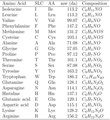
2.1. Molecular Biology
Figure 2.2: Orbitrap Mass Spectrometer molecule and a new radical cation. [61]
2.1. Molecular Biology
Figure 2.3: Mass Spectrometry Example
2.1.7.
High-resolution
Isoelectric
Focusing
Liquid
Chromatography Mass Spectrometry
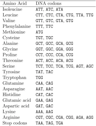
Branca et al.presented aLC-MS30-based method permitting unbiased genome-wide discovery of protein-coding loci in higher eukaryotes. Branca et al. used HiRIEF at
the peptide level in the [3.7,5.0] pH31 range and accurate peptide pI32 prediction [15] in combination with experimental prefractionation based on peptide pIand theoretical prediction ofpIto achieve search-space reduction. Lysates prepared from human A0431 cells and mouse N2A cells were digested with trypsin, and the resulting peptide samples were prefractionated using HiRIEF gel strips, each divided into 72 fractions [15].
Branca et al. evaluated the HiRIEF performance in a conventional search against the reference proteome, identifying 13,078 and 10,637 proteins in human and mouse, respectively [15].
30Liquid Chromatography Mass Spectrometry
31Hydrogenic Potential
2.1. Molecular Biology
‘Novel-only’ target/decoyanal ysi s (5% FDR)
2.1. Molecular Biology
2.1.8.
Peptide Sequence Problem
The Peptide Sequence Problem is the target of this research. In Peptide Fragmentation we explain how the chemical process works, and in Section 2.1.8.2, Definition we address the problem in a formal way. We present some others de novo
solutions in Section 2.1.8.2, Definition, and Section 2.1.8.3, Spectrum Graphs.
Important note:
The Peptide sequence problem is the target of this research.
2.1.8.1. Peptide Fragmentation
An amino acid unit in a peptide is called residue [48; 73] . When forming the
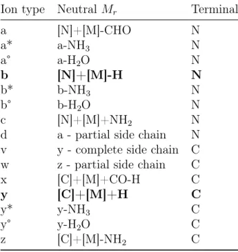
peptides bonds, an ionised amino acid molecule loses an Oxygen and two Hydrogen atoms. The result of this process is that the mass of the ionised molecule have 18da 33 more than theresidue [23]. The structure of both structures is shown in Figure 2.6, Peptide Residues. In Figure 2.5, Peptide Fragmentation, we present how the peptide fragmentation takes place. The red section corresponds to a C-terminal ion because the last atom is a C and the blue section corresponds to a N-terminal because the first atom is a N.
These are the generally accepted rules forMS/MSsequencing. For further reference, please go t [66].
Loss of Ammonia and Water:
1. Loss of Ammonia: y andb ion fragments containing the amino acid residuesR, K, Q, and N may appear to lose ammonia (NH3,−17da) [66].
2. Loss of Water: y and b ion fragments containing the amino acid residues S, T, and E may appear to lose water (H2O, −18da). In the case of Amino Acids, E must be at the N-terminusof the fragment for this observation to be made [66].
33Atomic mass unit (amu;dalton): A unit of mass equal to exactly 1
12 the mass of oneCatom, or
2.1. Molecular Biology
Ion type Neutral Mr Terminal
a [N]+[M]-CHO N
a* a-NH3 N
a° a-H2O N
b [N]+[M]-H N
b* b-NH3 N
b° b-H2O N
c [N]+[M]+NH2 N
d a - partial side chain N v y - complete side chain C w z - partial side chain C
x [C]+[M]+CO-H C
y [C]+[M]+H C
y* y-NH3 C
y° y-H2O C
z [C]+[M]-NH2 C
Table 2.3: Peptide Fragmentation Ion types
2.1. Molecular Biology
Figure 2.5: Peptide Fragmentation (from [23])
D y n a m ic P r o g r a m m in g A p p r o a c h t o P e p t id e S e q u e n c in g 1 7
|
| H
| H
|| O N C C
-R
(b) (a)
H |
| N C C
-| H
|| H O
O
R |
H
+
-Figure 2.6: Peptide Residues: (a) is the ionised amino acid and (b) is theresidue(from
[23])
Spectral Intensity Rules:
1. b ion intensity will drop when the next residue isP,G or alsoH, K, and R [66].
2. Internal cleavages can occur atPand Hresidues. An internal cleavage fragment is
a fragment that appears to be a shortened peptide with P and or H at its amino
terminus; e.g. the peptide EFGLPGLQNK may display the b ions PGLQNK, PGLQN, PGLQ, etc. These are the result of a double cleavage event. The y ion intensity will often be the most prominent peak in the spectrum [66].
2.1. Molecular Biology
Figure 2.7: Peptide SWRtandem mass spectrometry (from [23]) orR are encountered in the sequence [66].
4. When a cleavage appears before or afterR, the−17da(loss of ammonia) peak can be more prominent than the corresponding y orb ion [66].
5. When encountering Amino Acids in a sequence, the ion series can die out [66].
Amino Acid Composition:
1. It is possible to observe immonium ions at the low end of the spectrum that can give a clue to the amino acid composition of a peptide. One caveat is that if you do not see an immonium ion for an amino acid, this does not mean that that amino acid is absent from the sequence [66].
Isobaric Mass:
1. Amino Acids and Amino Acids have isobaric masses 34 35 and cannot be
34 Two (or more) ions are isobaric if they have the same nominal mass but different exact mass.
For example positive radical ions of N2, CO, and C2H4all have nominal mass of28da. However, their
exact (monoisotopic) masses are28.00559da,27.99436da, and28.03075daunits respectively [163].
35Monoisotopic, A spectrum containing only ions made up of the principal isotopes of atoms making
2.1. Molecular Biology
differentiated in a low energy collision. When we see this mass difference in a spectrum, we will label it X orLxx, adopting the Hunt [62] nomenclature [66].
2. Amino Acids and Amino Acids have near isobaric masses, 128.09496da and 128.05858da respectively. The delta mass is 0.03638da; this difference can be used to differentiate K from Q on a mass spectrometer capable of higher mass accuracy and resolution, such as a q-TOF mass spectrometer. Usually triple
quadrupole or ion trap mass spectrometers are incapable of this feat. On a lower mass accuracy mass spectrometers an acetylation can be performed to shift the mass of lysine by 42da. It can be assumed that a 128da mass shift internally on a tryptic peptide is a Glutamine unless followed by a Proline or sometimes Aspartic Acid [66].
3. There are instances where two residues will nearly equal the mass of a single residue, or a modified residue will nearly equal the mass of another amino acid [66].
More Rules:
1. When starting a de novo sequencing project, start at the high mass end of the
spectrum; the lower number of peaks at this end often makes it easier to start sequencing.
2. The region 60u below the parent mass can be confounded by multiple water and ammonia losses, be careful. Realise thatAmino Acidsmay be the first amino acid and may fall in this region [66].
2.1. Molecular Biology
4. The b1 fragment is seldom observed making it difficult to determine the order of the first two N-terminal amino acids in a peptide sequence. Solutions for this problem can include a one step Edman degradation or an acetylation [66].
2.1.8.2. Definition
Bandeira et al. [8] presented thePeptide sequence problem:
Definition 2.1.8.1. Bandeira et al. Spectrum:
s=s1, s2, s3, . . . , sn where si ∈2 ∀1≤i≤n (2.1)
Definition 2.1.8.2. Bandeira et al. Peptide:
π =π1, π2, π3, . . . , πn where si ∈2 ∀1≤i≤n (2.2)
Definition 2.1.8.3. Bandeira et al. Probability of peptide π generating spectrum s:
P(s|π) =
n
Y
i=1
P(si|πi) where P(x|y) is a 2×2 matrix (2.3)
2.1.8.3. Spectrum Graphs
Important note:
Spectrum Graphs is one technique used to solve approach the Peptide sequence problem.
Definition 2.1.8.4. NC-spectrum graph:
Given the mass W of a target peptide sequence P, k ions I1, . . . , Ik of P, and,
the masses w1, . . . , wk of those ions. Chen et al. presented the NC-spectrum graph
G = (V, E). For each Ij is not know if it is a N-terminal or a C-terminal. If Ij
is C-terminal ion, it has a complementary IC
2.1. Molecular Biology
where the 2 Dalton comes from the 2 extra Hydrogen atoms of the y-ion. The nodes
Nj and Cj are added to V to represent theIj and IjC where one of them is N-terminal
and the other one is C-terminal. Also nodes N0 and C0 area added to V to denote
the whole peptide mass.
V ={N0, N1, . . . , Nk, C0, C1, . . . , Ck} (2.4)
Every node of v ∈ V is placed in the real line using cord:V → R function defined
as follows: directed edge from x toy denoted by (x, y)and E(x, y) = 1, if the following conditions
2.1. Molecular Biology
(x, y)∈E if
x < y
x and y are not been generated by the same Ij
cord(y)−cord(x) is equals to total mass of an amino acid
(2.6)
In Figure 2.8, SWR Peptide Spectrum Graph there is an example where the path
N0−C2−N1−C0 contains exactly one of every pair of complementary nodes derived from the same ion, the spectrum corresponds to the original peptide SWR.
2.1.8.4. Peptide Sequence Problem
Definition 2.1.8.5. Chen et al. Edge scoring function: The nodes of V can be listed from left to right according to their coordinates asx0, x1, . . . , xk, y0, y1, . . . , yk; where xi
andyi are complementary. But, in practice a MS/MS may contain noise as mass peaks
of other types of ions from the same peptide, also mass peaks from unknown ions. Chen
et al. proposed a way to deal with this problem by using a predefined edge (and node) functions(·)function such that node corresponding to high peaks and edges labelled with
a single amino acid receive a higher scores. And the score of a path is defined as the
sum of the scores of the edges (and the nodes) of the given path [23].
Definition 2.1.8.6. Chen et al. Peptide sequence problem: For a given NC-Spectrum
graph G = (V, E), and a edge scoring function s(·), asks for the maximum score path fromx0 to y0, such that at most one of xj and yi for every 1≤i≤k is on the path.
Definition 2.1.8.7. Chen et al. Mass array: Let h the maximum mass under
construction. Let δ be the measurement precision. A mass arrayA :R→2is function
2.1. Molecular Biology
A(m) =
1 ∃π ∈Π where m=mw(π)
0 otherwise
(2.7)
Theorem 2.1.8.1 (Chen et al.: Theorem 1). The construction of A will take O(hδ)
time and for a given spectrum of k mass peaks, G can be constructed in O(k2) time.
This theorem was proven by the Theorem 1 of Chen et al. paper [23].
Definition 2.1.8.8. Chen et al. Ideal peptide sequence problem: is equivalent to the
problem which, given G= (V, E), asks for a directed path fromx0 toy0 which contains on of xi and yi for each i >0 [23].
Listed the nodes of G from left to right as x0, x1, . . . , xk, yk, . . . , y1, y0. Let M(i, j)
a (k+ 1)×(k+ 1) matrix with 0≤i, j ≤k. Let M(i, j) = 1 if and only if in G, there
is a path L from x0 to xi and a path R frin yj to y0, such that L∪R contains exactly
onf of xp and yp fir every p∈[1, i]∪[1, j]. Denoted the two path L∪R as LR path for
M(i, j) = 1. Let M(i, j) = 0 otherwise [23].
M(i, j) =
1 ∃L=x0− · · · −xi, R=yi− · · · −x0 where ∃!xp, yp∀p∈[1, i]∪[1, j]
0 otherwise
(2.8)
Theorem 2.1.8.2 (Chen et al.: Theorem 2). Given G = (V, E), the following statements hold:
1. Algorithm 1, Chen et al.: Compute-M(G) computes the matrix M in O(|V|2)
time.
2. Given M, a feasible solution of G can be found in O(|V|) time.
2.1. Molecular Biology
Algorithm 1 Chen et al.: Compute-M(G)
1: procedure Compute-M(G)
2: M(0,0)←1
3: M(i, j)←0∀i6= 0 orj 6= 0
4: for j = 2 to k do
5: for i= 0 toj −2do
6: if M(i, j−1) = 1 and E(xi, xj) = 1 then
7: M(j, j−1)←1
8: if M(i, j−1) = 1 and E(yj, yj−1) = 1 then
9: M(i, j)←1
10: if M(j−1, i) = 1 and E(xj−1, xj) = 1 then
11: M(j, i)←1
12: if M(j−1, i) = 1 and E(yj, yi) = 1 then
13: M(j−1, i)←1
4. All feasible solutions ofGcan be found inO(|V|2+n|V|)time andO(|V|2+n|V|)
space; where n is the number of solutions.
Also Chen et al. proposed a method to reduce the time and space complexities of Algorithm 1, Chen et al.: Compute-M(G). M can be encoded in two linear arrays
Definition 2.1.8.9(Chen et al.: cross edges and inside edges). Define an edge(xi, yj)
with 0≤i, j ≤k to be a cross edge, and edge xi, xj or (yi, yj) with 0≤i < j ≤k to be
a inside edge. Let lce(z) (lce:V →N) be the length of the longest consecutive inside
edges starting from node z, i. e.,
lce(xi) =j −i if E(xi, xi+1) =· · ·=E(xj−1, xj) = 1 and (j =k or E(xj, xj+1) = 0)
lce(jj) =j−i if E(yj, yj−1) =· · ·=E(jj+1, yi) = 1 and (i= 0 or E(yi, xi−1) = 0) (2.9)
2.1. Molecular Biology
Algorithm 2 Chen et al. Compute-Q(G)
1: procedure Compute-Q(G)
2: Q(i, j)←0∀0≤i, j ≤k
3: for j = 1 to k do
4: if E(yj, y0) = 1 then
5: Q(0, j)←max{Q(0, j), s(yj, y0)}
6: if E(x0, xj) = 1 then
7: Q(j,0)←max{Q(j,0), s(x0, xj)}
8: for i= 1 toj −1do
9: for E(yj, yp) = 1 and Q(i, p)>0do
10: Q(i, j)←max{Q(i, j), Q(i, p) +s(yj, yp)}
11: for E(cp, xj) = 1 and Q(p, i)>0 do
12: Q(i, j)←max{Q(j, i), Q(p, i) +s(xp, xj)}
Definition 2.1.8.10. One-amino acid modification problem: is equivalent to the problem which given G= (V, E), asks for two nodes vi and vj, such that E(vi, vj) = 0,
but adding the edge to G creates a feasible solution that contains the edge.
LetN(i, j) a(k+ 1)×(k+ 1) matrix with0≤i, j ≤k. LetN(i, j) = 1 if and only if in G, there is a path from xi toyj which contains exactly one of xp and yp for every
p∈[1, i]∪[1, j]. Let N(i, j) = 0 otherwise [23]. Algorithm 3 Chen et al. Compute-N(G)
1: procedure Compute-N(G)
2: N(i, j)←0∀0≤i, j ≤k
3: Compute N(k, k−1)
4: Compute N(k−1, k)
5: for j =k−2 to 0do
6: for i=k toj + 2 do
7: if N(i, j+ 1) = 1and E(xi, xj) = 1 then
8: N(j, j+ 1)←1
9: if N(i, j+ 1) = 1and E(yj+1, yj) = 1 then
10: N(i, j)←1
11: if N(j+ 1, i) = 1 and E(xj, xj+1) = 1 then
12: N(j, i)←1
13: if N(j+ 1, i) = 1 and E(yi, yj+1) = 1 then
2.1. Molecular Biology
Theorem 2.1.8.5 (Chen et al.: Theorem 7). Given G = (V, E), the following statements hold:
1. Algorithm 3, Chen et al. Compute-N(G) computes the matrix N in O(|V|2)time.
2. All possible amino acid modifications can be found in O(|V||E|)time andO(|V|2)
2.2. Mathematical Fundamentals
A1 R1
R2 M1
M2
M3 Y1
Y2
Y3
Y4 M4
M5
M6
M7 A2
A3
A4 T1
T2 H1
Figure 2.9: Army math net/lattice Original figure was taken from [113]
2.2.
Mathematical Fundamentals
This particular section is a collection of many fields of Mathematics. Most of these topics are studied as a part of Computer Science and Mathematics college courses. We present Set Theory, Algebraic Structures, and Topology. This section intends is to provide the reader quick access to the definitions all along this document.
2.2.1.
Set Theory
These are the well known definitions of the Set theory, for further information the reader can refer to [45; 141].
Definition 2.2.1.1 (poset). Partially ordered set
Aposetis defined as a pair(X,≤)whereX is anon-emptyset and· ≤ ·:X×X →
2 is a binary relation over X that satisfies for all a, b, c∈X:
PO1 Reflexive: a≤a
PO2 Anti-symmetry: a≤b∧b≤a =⇒ a=b
PO3 Transitivity: a≤b∧b≤c =⇒ a≤c
Definition 2.2.1.2 (net). A net is aposetwith an additional axiom for alla, b, c∈X:
2.2. Mathematical Fundamentals
N2 Anti-symmetry: a≤b∧b ≤a =⇒ a =b
N3 Transitivity: a≤b∧b ≤c =⇒ a≤c
N4 : ∃m∈X m≤a∧m ≤b
In Figure 2.9,Army math net/lattice there is an example of net
Definition 2.2.1.3 (ordered set). An ordered set is a poset with an additional axiom for all a, b, c∈X:
O1 Reflexive: a≤a
O2 Anti-symmetry: a≤b∧b ≤a =⇒ a =b
O3 Transitivity: a≤b∧b ≤c =⇒ a≤c
O4 Totality: a≤b∨b ≤a
Definition 2.2.1.4(Subsets). 2K: The set of all the subsets of a given setK is denoted
as:
2K ={k where k ⊂K} (2.11)
Definition 2.2.1.5 (string). Σ∗: The set of all strings of a given known as the alphabet
Σ is denoted as:
Σ∗ = [
i∈N0
Σi (2.12)
Σ0 ={λ} (2.13)
2.2. Mathematical Fundamentals
An element ofΣ∗ is known as astringof theΣalphabet. λis a symbol that represents an empty string, also |λ|= 0.
2.2. Mathematical Fundamentals
2.2.2.
Algebraic Structures
In Algebra, arithmetical operations and formal manipulations are applied to abstract symbols rather than specific numbers [35]. These are the well known concepts of Abstract Algebra. The reader can refer to [76; 114] for further information.
Definition 2.2.2.1 (monoid). A monoid is an algebraic structure with a single
associative binary operation and an identity element. For a given set S and a binary
operation ·:S×S →S the pair (S,·) is monoid if for all a, b∈S stands:
M1 Associative: (a·b)·c=a·(b·c)
M2 Neutral element: ∃e∈S e·a=a=a·e
Definition 2.2.2.2 (commutative monoid). A commutative monoid is an algebraic structure with a single associative binary operation and an identity element. For a
given set S and a binary operation ·:S×S→S the pair (S,·) is commutative monoid if for all a, b∈S:
CM1 Associative: (a·b)·c=a·(b·c)
CM2 Commutative: a·b=b·a
CM3 Neutral element: ∃e e·a=a=a·e
Definition 2.2.2.3 (semi ring). For a given set R and two binary operation + :R×
R → R, known as addition, and, · : R×R → R, known as multiplication, the tuple
(R,+,·) is a semi ring if for all a, b, cinR:
SM1 : (R,+) is a commutative monoid with neutral element 0
SM2 : (R,·) is a monoid with neutral element 1
2.2. Mathematical Fundamentals
a·(b+c) = (a·b) + (a·c)
(b+c)·a= (b·a) + (c·a)
SM4 Multiplication by 0 annihilates R: 0·a=a·0 = 0
Remark. : (N0,+,·) is a semi ring.
Definition 2.2.2.4(field). For a given setF and two binary operations+ :F×F →F, known as addition, and, ·:F ×F →F, known as multiplication; the tuple (F,+, c˙) is a field if the the for all a, b, c∈F:
F1 Associativity of addition: (a+b) +c=a+ (b+c)
F2 Associativity of multiplication: (a·b)·c=a·(b·c)
F3 Commutativity of addition: a+b=b+a
F4 Commutativity of multiplication: a·b =b·a
F5 Addition neutral: ∃0∈F a+ 0 =a= 0 +a
F6 Multiplication neutral: ∃1∈F a·1 =a = 1·a
F7 Addition inverse: ∃ −a a+ (−a) = 0
F8 Multiplication inverse: ∃a−1 a·a−1 = 1
F9 Distributivity of multiplication over addition: a·(b+c) = a·b+a·
Definition 2.2.2.5 (homomorphism). If f :A→B is a map between two (A,·),(B,·)
algebraic structures of the same type that preserves the operations of the structures:
2.2. Mathematical Fundamentals
Definition 2.2.2.6 (generation set). For a given algebraic structure G, a generation
set S⊂G is a subset such that every element of G can be expressed as the combination
(under the Goperations), of finitely many elements of S. If S is finite, then a groupG
= hSi is called finitely generated. The elements of S are called generators.
Definition 2.2.2.7(Cayley Graph). Suppose that GG is a group andS is ageneration
set. The Cayley graph Γ = (G, S) is a coloured directed graph constructed as follows:
Each element g ∈G assigned a vertex g ∈V(Γ).
Each generator s ∈S is assigned a colour cs.
For any g ∈G, s∈S, there is an edge (g, gs)∈E(Γ) with colour cs.
The details of this structure can be found on [20; 21].
In Figure 2.10, Example of Cayley Graph there is an example of a Cayley Graph for a string with only 4 characters.
Definition 2.2.2.8 (lattice). An algebraic structure (L,∨,∧), consisting of a setLand
two binary operations ∨ : L×L → 2, and ∧ : L×L → 2 with following axiomatic
identities holds for all a, b, c∈L:
LT1 Commutative laws:
a∨b=b∨a
a∧b=b∧a
LT2 Associative laws:
a∨(b∨c) = (a∨b)∨c
a∧(b∧c) = (a∧b)∧c
2.2. Mathematical Fundamentals
a∨(a∧b) = a
a∧(a∨b) = a
LT4 Idempotent laws:
a∨a=a
a∧a=a
Further material related to lattices can be found on [47; 54].
Definition 2.2.2.9(bounded lattice). Abounded latticeis an algebraic structure of the form (L,∨,∧,0,1)such that(L,∨,∧) is alattice, 0(the lattice’s bottom) is the identity element for the join operation ∨, and1 (the lattice’s top) is the identity element for the
meet operation ∧.
LT5 Identity laws:
a∨0 =a
a∧1 =a
Definition 2.2.2.10 (complemented lattice). A complemented lattice is a bounded
lattice, in which every element a has a complement unary operation¬, i.e. an element
¬a such that:
LT6 Complement laws:
a∨ ¬a= 1
a∧ ¬a= 0
Definition 2.2.2.11 (Boolean space). A Boolean space is of a complemented lattice
2 = ({0,1},∨,∧,0,1,¬) with a distribution law for all a, b, c∈2:
2.2. Mathematical Fundamentals
a∨(b∧c) = (a∧b)∨(a∧c)
a∧(b∨c) = (a∨b)∧(a∨c)
Definition 2.2.2.12 (Vector space). FR: For a given field (F,+,·) known as the field
and a natural number R∈N known as the rank:
FR =
F R = 1
F ×FR−1 R >1
(2.19)
Definition 2.2.2.13 (~0). zero of a Vector space: for a given FR Vector space on the
field (F,+,·):
h~0ij =neutral(+) ∀j ∈N,1≤j ≤R (2.20)
Definition 2.2.2.14 (The inth basis of a Vector space). 1~i: for a given FR Vector
space on the field (F,+,·), i∈N, i≤R:
h1~iij =
neutral(+) i6=j
neutral(·) i=j
∀j ∈N,1≤j ≤R (2.21)
Definition 2.2.2.15 (The basis of a Vector space). ˜1: for a given FR Vector space on
the field (F,+,·):
˜
2.2. Mathematical Fundamentals
2.2.3.
Topology
Figure 2.11: Example of Continuous Transformations
The classical example of Topology is the transformation of a mug in a toroid. Image taken from [162].
2.2. Mathematical Fundamentals
parts [41]. An example of this can be observed in Figure 2.11, Example of Continuous Transformations, where a mug can be deformed into a toroid 36.
Important note:
The main topics of interest in Topology are the properties that remain unchanged by such continuous deformations
These are well known definitions and theorems of Topology Theory; most of these definitions and theorems are referenced in [29]. For further information the reader can refer to [70; 152; 153; 154; 155; 156].
Definition 2.2.3.1 (Topological space). A topological space is an ordered pair (X, τ), where X is a set and τ ⊂ 2X is a collection of subsets of X, satisfying the following
axioms:
1. X ∈τ and ∅ ∈τ;
2. For any index I over τ: ∪i∈IUi ∈τ;
3. For any U, V ∈τ the intersection U ∩V ∈τ
τ is known as the open sets ofX.
There is particular kind ofTopological space, the metric spaces; where the open sets
are defined as follows.
Definition 2.2.3.2 (metric space). A non-empty set X with a map d:X×X →R is called a metric space if the map d has the following properties [29]:
MS1 : d(x, y)≥0|∀x∈X∀y ∈X
MS2 : d(x, y) = 0 ⇐⇒ x=y
MS3 : d(x, y) = d(y, x)∀x∈X∀y∈X
36 A surface of revolution obtained by rotating a closed plane curve about an axis parallel to the
2.2. Mathematical Fundamentals
MS4 : d(x, y)≥d(x, z) +d(z, y)|∀x∈X∀y∈X∀ ∈X
The map d is called the metric on X or sometimes the distance function on X. The phrase “(X, d)is a metric space” means that d is a metric on the set X. Property MS4 is often called the triangle inequality [29; 133].
Definition 2.2.3.3 (distance defined by a function). For a given function f :X →R, and i∈N let the df :X×X →R+0 the distance defined by f as:
df(a, b) = |f(a)−f(b)| (2.23)
Definition 2.2.3.4 (equivalent class of a function). For a given sets X, Y, and a function f :X →Y, the equivalent class [x]f are defined as:
[y]f ={x∈X|f(x) =y}∀y ∈f(X) (2.24)
And all the equivalent classes[X]f as:
[X]f ={[f(x)]f∀x∈X} (2.25)
Theorem 2.2.3.1. ([X]f, df) is ametric space For any given non-empty set X, and
a function f :X →R; ([X]f, df) is a metric space.
Proof. For all [x]f,[y]f,[z]f ∈[X]f:
MS1 The codomain of df is R+0 by definition.
MS2 ⇐:
df([x]f,[x]f) =|x−x|= 0 (2.26)
⇒:
2.2. Mathematical Fundamentals
MS3
df([x]f,[y]f) =|x−y|=|y−x|=df([y]f,[x]f) (2.28)
MS4
df([x]f,[z]f) = |x−z| (2.29)
=|x−y+y−z| (2.30)
≤ |x−y|+|y−z| (2.31)
=df([x]f,[y]f) +df([y]f,[z]f) (2.32)
Definition 2.2.3.5 (ball). in a metric space
For a given metric space (E, d), a point p∈E and a radius r∈R+, the (open) ball B(p;r) is defined as
B(p;r) ={q∈E|d(p, q)< r} (2.33)
Definition 2.2.3.6 (open set). in a metric space
For a given metric space (E, d), A⊂E is an open set if and only if:
∀p∈A∃r∈R+|B(p;r)⊂A (2.34)
The ∅ and E are open sets by definition.
Definition 2.2.3.7 (neighbourhood). of a set in a metric space
If A 6= ∅ ∈ E, an open neighbourhood of A is an open set that contains A. If
A={p}, we can speak of the open neighbourhood of p (instead of the set{p}).
2.2. Mathematical Fundamentals
Definition 2.2.3.9 (closed set). in a metric space For a given metric space (E, d),
K ⊂E is an closet set if and only if E−K is an open set.
Definition 2.2.3.10 (cluster point). of a set
A cluster point of A ⊂ E is a point p ∈ E that every neighbourhood has a non-empty intersection with A. All the cluster points of A are denoted as A¯.
Definition 2.2.3.11 (continuous mapping). Let (E, d) and (E0, f d0) two metric
spaces. A mapping f : E → E0 is said to be continuous at point x0 ∈ E if, for every
neighbourhood of V0 of f(x0) ∈ E‘ there is a neighbourhood V of x0 such that f(V)⊂V0. f is said to be continuous in E (or simple continuous) if it is continuous at every point of E.
In order to be continuous atx0 ∈E, a necessary and sufficient condition is that for
every neighbourhood V0 of f(x0) in E0, f−1(V0) be a neighbourhood of x0 ∈E.
Another, necessary and sufficient condition (only for metric spaces) is that:
∀ >0 ∃δ >0 d(x0, x)< δ =⇒ d0(f(x0), f(x))< (2.35)
And all of these properties are equivalent:
1. f is continuous;
2. for every open set U0 in E0, f−1(U0) is open set in E;
3. for every closed set K0 in E0, f−1(K0) is closed set in E;
4. for every open set A in E, f( ¯A)⊂f(A).
Definition 2.2.3.12 (lower semi-continuous mapping). We say that f is lower
semi-continuous at x0 if for every > 0 there exists a neighbourhood U of x0 such that
2.2. Mathematical Fundamentals
towards x0 when f(x0) = +∞. Equivalently, in the case of a metric space, this can be
expressed as:
lim inf
x→x0
f(x)≥f(x0) (2.36)
where lim inf is the limit inferior (of the function f at point x0).
Definition 2.2.3.13 (limit). of a function Let (E, d) be a metric space, A ⊂ E, a a
cluster point of A. Suppose that a 6∈ A. If f is a mapping of A in to a metric space
E0. we say that f(x) has a limit a0 ∈E0 where x ∈A tends to a. It the mapping g of
A∪a ⊂ E0 defined by taking g(x) = f(x) for every x ∈ A, g(a) = a0, is continuous
mapping at point a. It is denoted as:
lim
x→a,x∈Af(x) (2.37)
In order that a0 ∈ E0 be a limit of f(x) when x ∈ A tends to a, a necessary and
sufficient condition is that, for every neighbourhood V0 of a0 in E0, there exists a
neighbourhood V of a in E such that f(V ∩A)⊂V0.
Another (only for metric spaces), necessary and sufficient condition is that:
∀ >0 ∃δ >0 x∈A, d(x, a)< δ =⇒ d0(a0, f(x))< (2.38)
Definition 2.2.3.14 (Cauchy sequence). In a metric space (E, d) a Cauchy sequence is a infinte sequence {xn} such that:
2.3. Computer Science
2.3.
Computer Science
As part of the review of the state of the art, we present some examples of how the techniques presented inMathematical Fundamentals, especiallyTopology, were applied in Computer Science to solve similar problems.
Important note:
These techniques were not applied to this research, but they were considered. This section intends to be illustrative.
2.3.1.
Nearest Neighbour Search
The problem of theNNSconsists in given a setS of pointsndata points in ametric space X (see item 2.2.3, Topology); the task is to process these points so that, given a
query point q∈X the data nearest to q can be reported quickly [7].
2.3.1.1. Space Partitioning
Space partitioning is one of NNS techniques where the search space is divided
recursively and the search time is usually in order of O(log(n)) (where n is the number elements in the search space).
2.3.1.2. R-Tree
2.3. Computer Science
R1
R3
R4 R9
R11
R13
R10
R12
R16
R15
R14 R8
R2
R6
R7 R17
R18
R19 R5
R1 R2
R3 R4 R5 R6 R7
R8 R9 R10 R11 R12 R13 R14 R15 R16 R17 R18 R19
2.3. Computer Science
2.3.2.
Locality Sensitive Hashing
LSH37is a family of techniques that reduces the dimensionality of high-dimensional data. The techniques ofspace partitioning work very well for scalar and vectorial values
where the dimensionality is low. But, in documents, this approach is not so effective. Rajaraman and Ullman mentions that the most effective way to represent documents as sets, for the purpose of identifying lexically similar documents is to construct from the document the set of short strings that appear within it [118].
2.3.2.1. Jaccard Similarity of Sets
Definition 2.3.2.1. The Jaccard index, also known as the Jaccard similarity
coefficient, is a statistic used for comparing the similarity and diversity of sample sets. The Jaccard coefficient measures similarity between finite sample sets, and is defined as the size of the intersection divided by the size of the union of the sample sets [118]:
J(A, B) = |A∩B|
|A∪B| (2.40)
In the case when A and B are both empty the value is 1: J(∅,∅) = 1 [118].
Definition 2.3.2.2. The Jaccard distance, is complementary to the Jaccard similarity
coefficient, and it can be defined as [118]:
dJ(A, B) = 1−J(A, B) =
|A∪B| − |A∩B|
|A∪B| (2.41)
2.3.2.2. Min Hash
Min hashis a technique that takes a document as a string of characters. It defines ak-shingle for a document to be any sub-string of lengthk found within the document. Then, associating with each document, the set of k-shingles that appear one or more
2.3. Computer Science
times within that document [118].
The probability that the minhash function for a random permutation of rows

![Figure 2.2: Orbitrap Mass Spectrometer molecule and a new radical cation. [61]](https://thumb-us.123doks.com/thumbv2/123dok_es/3730947.642436/45.918.151.813.106.583/figure-orbitrap-mass-spectrometer-molecule-and-radical-cation.webp)

![Figure 2.4: HiRIEF diagram (taken from [15])](https://thumb-us.123doks.com/thumbv2/123dok_es/3730947.642436/47.918.148.792.258.881/figure-hirief-diagram-taken-from.webp)
![Figure 2.5: Peptide Fragmentation (from [23]) D y n a m i c P r o g r a m m i n g A p p r o a c h t o P e p t i d e S e q u e n c i n g 1 7 | | H H| O|| N C C -R (b)(a)H| - N - C - C -|H|H O||ORH|+](https://thumb-us.123doks.com/thumbv2/123dok_es/3730947.642436/50.918.112.777.102.680/figure-peptide-fragmentation-d-p-p-s-orh.webp)
![Figure 2.7: Peptide SWR tandem mass spectrometry (from [23]) or R are encountered in the sequence [66].](https://thumb-us.123doks.com/thumbv2/123dok_es/3730947.642436/51.918.149.814.103.458/figure-peptide-swr-tandem-mass-spectrometry-encountered-sequence.webp)
![Figure 2.8: SWR Spectrum Graph (from [23])](https://thumb-us.123doks.com/thumbv2/123dok_es/3730947.642436/54.918.107.775.104.414/figure-swr-spectrum-graph-from.webp)
