Near-infrared photometry of globular clusters towards the Galactic bulge:
observations and photometric metallicity indicators
Roger E. Cohen,
1‹Christian Moni Bidin,
2Francesco Mauro,
1,3Charles Bonatto
4and Douglas Geisler
11Departamento de Astronom´ıa, Universidad de Concepci´on, Casilla 160-C, Concepci´on, Chile
2Instituto de Astronom´ıa, Universidad Cat´olica del Norte, Av. Angamos 0610, Casilla 1280, Antofagasta, Chile 3Instituto Milenio de Astrof´ısica, Santiago, Chile
4Departamento de Astronomia, Universidade Federal do Rio Grande do Sul, Av. Bento Gonc¸alves 9500 Porto Alegre 91501-970, RS, Brazil
Accepted 2016 September 23. Received 2016 September 21; in original form 2015 December 7
A B S T R A C T
We present wide-fieldJHKSphotometry of 16 Galactic globular clusters located towards the
Galactic bulge, calibrated on the Two Micron All-Sky Survey photometric system. Differ-ential reddening corrections and statistical field star decontamination are employed for all of these clusters before fitting fiducial sequences to the cluster red giant branches (RGBs). Observed values and uncertainties are reported for several photometric features, including the magnitude of the RGB bump, tip, the horizontal branch (HB) and the slope of the upper RGB. The latest spectroscopically determined chemical abundances are used to build distance- and reddening-independent relations between observed photometric features and cluster metallic-ity, optimizing the sample size and metallicity baseline of these relations by supplementing our sample with results from the literature. We find that the magnitude difference between the HB and the RGB bump can be used to predict metallicities, in terms of both iron abundance [Fe/H] and global metallicity [M/H], with a precision of better than 0.1 dex in all three near-IR bandpasses for relatively metal-rich ([M/H]−1) clusters. Meanwhile, both the slope of the upper RGB and the magnitude difference between the RGB tip and bump are useful metallicity indicators over the entire sampled metallicity range (−2 [M/H]0) with a precision of 0.2 dex or better, despite model predictions that the RGB slope may become unreliable at high (near-solar) metallicities. Our results agree with previous calibrations in light of the relevant uncertainties, and we discuss implications for clusters with controversial metallicities as well as directions for further investigation.
Key words: globular clusters: general – infrared: stars.
1 I N T R O D U C T I O N
Galactic globular clusters (GGCs) play a crucial role in constraining stellar evolutionary models as well as Galactic chemical evolution. Recently, many of these clusters have been the subject of large-scale photometric surveys using deep, high-resolution multicolour space-based observations (Piotto et al.2002; Sarajedini et al.2007; Piotto et al.2015). However, GGCs located towards the Galactic bulge, despite their importance as the most metal-rich (and in some cases, massive) members of the GGC system, have been generally excluded from these surveys due to severe total and differential extinction at optical wavelengths. For this reason, infrared (IR) wavelengths, where the effects of extinction are greatly reduced
E-mail:[email protected]
(AK ∼ 0.12AV; Casagrande & VandenBerg 2014), are ideal for
photometric investigations of such clusters.
The Vista Variables in the Via Lactea (VVV), a European South-ern Obseratory (ESO) public survey, has observed a 562 deg2field including the Galactic bulge and a portion of the disc inYZJHKS
filters down to KS∼ 20, and thus presents an ideal opportunity
cluster near-IR colour–magnitude diagrams (CMDs) and their chemical abundances, as these relations can then be applied to ob-tain photometric metallicity estimates. With an eye towards future application for distant and/or heavily extincted stellar systems, we revisit these calibrations. This is advantageous in light of not only the quality of the VVV photometry, but more importantly its wide-field nature, facilitating a statistical assessment of contamination by field stars (see Section 2.5), leveraged together with improved spectroscopic abundances (see Section 4.1) and reddening maps (e.g. Alonso Garcia et al.2012; Gonzalez et al.2012; Cohen et al. 2014, see Section 2.4). Here, we analyse an initial subset of GGCs within the VVV survey area that have spectroscopically measured [Fe/H] values, with the goal of constructing updated distance- and reddening-independent relations between photometric features ob-servable on the cluster giant and horizontal branches (HBs) and their metallicities. The resulting relations between distance- and reddening-independent photometric features measured from near-IR cluster CMDs versus cluster metallicities are further optimized by concatenating the results presented here with those available in the literature.
In the next section, we present the details of our observations and data processing, including corrections for differential reddening and field star contamination, and the resulting cluster CMDs. In Section 3, we describe our methodology for measuring cluster photometric features as well as their uncertainties, and in Section 4, we use these measurements, along with literature values, to construct relations that can be used to estimate metallicities of old stellar populations photometrically. In the final section, we summarize our results, discussing implications for clusters with controversial metallicity values.
2 DATA P R O C E S S I N G
2.1 Target cluster selection
There are 36 GGCs presently known in the area covered by the VVV survey according to the catalogue of Harris (1996, 2010 re-vision, hereafterH10), plus one candidate discovered as a result of this survey (VVV CL001; Minniti et al.2011). We aim to derive re-lations between observed photometric parameters on the cluster red giant branches (RGBs), where the most IR-bright cluster members lie, and cluster metallicities (in terms of both [Fe/H] and [M/H]), so we have selected a subset of the GGCs in the VVV survey area that all have spectroscopically measured [Fe/H] values. To restrict our sample to only those clusters with high-quality [Fe/H] mea-surements, we consider only clusters with a value of ‘1’ in the last column of table A1 in Carretta et al. (2009, hereafter C09), and add two clusters (NGC 6380 and M 28=NGC 6626) with recent spectroscopic [Fe/H] values based on CaIItriplet equivalent widths (Saviane et al.2012; Mauro et al.2014, hereafterM14), comprising a sample of 17 GGCs from VVV including photometry of NGC 6544 described in Cohen et al. (2014). We return to the issue of various spectroscopic metallicities for the target clusters in Section 4.1, and the use of literature measurements for additional clusters is discussed in Section 4.3.
2.2 Photometry
The images that we employ were obtained as part of the VVV sur-vey using the 4.1 m Visible and Infrared Sursur-vey Telescope for As-tronomy (VISTA), equipped with the VIRCAM (VISTA InfraRed Camera) instrument (Emerson, McPherson & Sutherland 2006).
The VIRCAM detector consists of a 4×4 array of chips, each with 2048×2048 pixels and a pixel scale of 0.339 arcsec per pixel. A description of the survey can be found in Minniti et al. (2011), with further details regarding the survey strategy and data products in Saito et al. (2010). Information regarding the first data release, including products that we employ here, is given in Saito et al. (2012). Point spread function-fitting (PSF) photometry is performed on VVV images obtained from the Cambridge Astronomical Survey Unit (CASU)1via the iterative usage of the
DAOPHOT/ALLFRAMEsuite
(Stetson 1987, 1994) identically to previous studies (e.g. Mauro et al.2012; Cohen et al.2014). This PSF photometry pipeline has been customized to operate on pre-processed, stacked VVV im-ages produced by CASU, and the reader is referred to Mauro et al. (2013) for a detailed description of the PSF photometry pipeline and comparisons with other data reduction techniques and products. We have chosen to perform photometric and astrometric calibration of the resulting catalogues to 2MASS for two reasons. First, be-cause our photometry becomes saturated below the tip of the RGBs of all of our target clusters, merging our photometric catalogues with 2MASS is necessary in order to construct fiducial sequences and luminosity functions (LFs) over the entire luminosity range of the cluster RGBs and measure photometric features (described in Section 3). Secondly, by performing our analysis in the 2MASS photometric system, our results may be directly compared and/or combined with previous near-IR studies, the majority of which have been calibrated to 2MASS as well (Valenti et al.2004a;V10; Chun et al.2010;V10; Cohen et al.2014,2015). To calibrate our photom-etry and astromphotom-etry to the 2MASSJHKSsystem, a magnitude range
is selected among the stars matched between VVV and the 2MASS point source catalogue (PSC) in which both data sets show good agreement with minimal scatter, avoiding stars that are sufficiently faint so as to be unduly affected by crowding and/or large photomet-ric errors in 2MASS. Additionally, stars with neighbours detected within 2.2 arcsec contributing a contaminating flux of≥0.03 mag are rejected from use as local standards (e.g. Mauro et al.2013). Instrumental magnitudes resulting from PSF photometry are cali-brated to the 2MASSJHKSsystem (rather than the native VISTA
filter system) using the classical transformation equations of the
formm2MASS−minst=a+b(J−KS)2MASS, whereais a
photomet-ric zero-point offset andbis a linear colour term. The coefficients
aand bare obtained independently for each VIRCAM chip per image per filter using least squares fitting, but using a weighting scheme to downweight discrepant data points2rather than a sigma clipping or rejection procedure. For the coefficientsaandb, the values measured in each of the three (J, H, KS) filters are a=
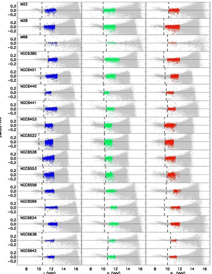
(0.62,0.26,−0.52)±(0.04,0.03,0.06) andb=(0.03,−0.02,−0.02) ±(0.02,0.02,0.02), compared to median fitting uncertainties≤0.02 for the offsetaand≤0.01 for the colour termbin all three band-passes. Thus, the resulting photometric calibrations have 1σ zero-point uncertainties of0.02 mag for all target clusters, and a star by star comparison between our calibrated photometry and 2MASS in all threeJHKSfilters is shown in Fig.1. All stars matched between
VVV and 2MASS are shown in grey in each panel of Fig.1, and
1Images and aperture photometry catalogues from VVV data releases are publicly available through the ESO archive, and CASU is located at
http://casu.ast.cam.ac.ck
Figure 1. A comparison between our calibrated magnitudes and those from 2MASS for all of our target clusters. Each cluster is shown as a row of three plots, illustrating the difference between VVV and 2MASS as a function of (left to right) VVVJ,HandKSmagnitude. In each plot, the grey points represent all
the subset of these stars used for calibration is overplotted. The vertical dashed line in each panel of Fig.1indicates the magni-tude at which the VVV photometry is unusable due to saturation, that varies somewhat from cluster to cluster due to differences in stellar crowding as well as observing conditions. For stars that are brighter than this limit in any of the threeJHKSfilters, we
supple-ment our VVV catalogues with photometry from the 2MASS PSC. All colours and magnitudes that we report in this study are in the 2MASS photometric system (rather than the native VISTA system), and additional discussions regarding the calibration of VVV pho-tometry to the 2MASS system can be found in Moni Bidin et al. (2011) and Chen´e et al. (2012).
Astrometric calibration is performed to the coordinates given in the 2MASS PSC, using the world coordinate system information placed in the headers of the stacked VVV images by CASU as an initial guess in order to correct for effects of geometric distortion. The resulting astrometry has a root mean square (rms) precision of ∼0.2 arcsec for all target clusters, in accord with the astrometric precision of 2MASS.
2.3 Comparison with previous photometry
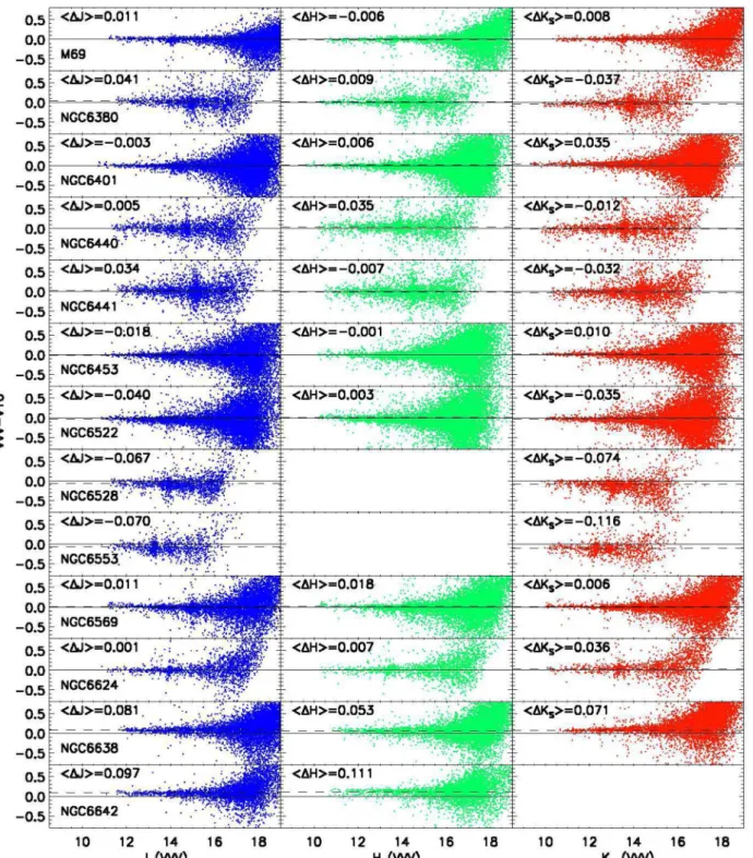
Of our target clusters, 13 of 16 are also included in the compilation ofV10.3We calculate the mean magnitude differences in each filter between our photometry and theirs using a weighted 2.5σ clip in magnitude bins, employing only unsaturated stars brightward of the observed LF peak. The resulting comparisons of magnitude difference as a function of magnitude are shown for each cluster in Fig.2. Given our photometric zero-point uncertainty of<0.02 mag and the zero-point uncertainty of 0.05 mag estimated byV10, the two studies, having both been calibrated to 2MASS, are generally in good agreement. While larger offsets are seen in a few cases (NGC 6528, NGC 6553, NGC 6638, NGC 6642), the direct comparison with 2MASS in Fig.1gives no reason to be doubtful about the calibration of these clusters. Specifically, the mean magnitude offset between the VVV and 2MASS photometry (weighted by the inverse square of their total photometric uncertainties) over the magnitude range of stars used for calibration is<0.016 mag inJandKSand
<0.023 mag inHfor these four clusters (these mean differences are
<0.02 mag for all other clusters in all bandpasses as well). Photometric analysis of GGCs towards the Galactic bulge can be severely hampered by contamination from field stars in the bulge and disc, particularly in cases where bulge and disc contami-nants are inseparable from the cluster evolutionary sequences using colour–magnitude criteria alone. Statistical field star decontamina-tion methods that compare the colour–magnitude loci of cluster and field stars generally rely on the assumption that reddening is spatially invariant (see Section 2.5.1 below), so before undertaking analyses of the GGC photometry, we first correct for differential reddening and then apply a statistical field star decontamination procedure.
2.4 Differential reddening
We correct our photometric catalogue of each cluster for redden-ing only in a strictly differential sense (we do not correct for total line-of-sight extinction). This is done using the reddening maps of
3See the Bulge Globular Cluster Archive athttp://www.bo.astro.it/∼GC/
ir_archive
Gonzalez et al. (2012),4adopting the value ofE(J−K
S)
correspond-ing to the location of the cluster centre as a reference zero-point for the differential reddening corrections over the spatial area of each cluster. This reference value is given asE(J−KS)REFin Table1. The photometric catalogue for each cluster is then corrected for reddening variations over the field of view using the difference between the value of E(J − KS) at a given spatial location and
E(J−KS)REF(i.e. the value at the spatial location of the cluster centre). However, since the Gonzalez et al. (2012) maps were con-structed by measuring the variation in the (J−KS) colour of the
Galactic bulge red clump (RC) as a function of spatial location, the number statistics necessary to reliably measure the bulge RC colour restrict the spatial resolution of the Gonzalez et al. (2012) maps to
>1 arcmin, while significant differential reddening towards bulge GGCs can occur on spatial scales of arcseconds (Alonso Garcia et al.2012; Massari et al.2012; Cohen et al.2014). Furthermore, the Gonzalez et al. (2012) maps were constructed from aperture photometry catalogues rather than PSF photometry, and therefore suffer from crowding and incompleteness significantly brightward of their detection limits as compared to PSF photometry (e.g. Mauro et al.2013, see their fig. 6). Therefore, where available, we have combined the Gonzalez et al. (2012) maps of the field surround-ing each cluster with high-spatial resolution reddensurround-ing maps (con-structed using cluster stars) of the central region of the cluster. The high-resolution maps were taken from Alonso Garcia et al. (2012) where available (eight clusters), from Cohen et al. (2014) in the case of NGC 6544, and for six more clusters, we employ maps similarly constructed from archival opticalHubble Space Telescopeimaging described in detail elsewhere (Cohen et al., in preparation).5While the high-resolution maps are generally restricted to the inner regions of the target clusters where the membership probability is high, we note that they extend well beyond the cluster half-light radii from the Harris (1996) andH10catalogue, encompassing the majority of cluster members.6These high-resolution maps are also applied in a strictly differential sense, relative toE(J−KS)REF, but we must take into account that the differential reddening corrections given by the Alonso Garcia et al. (2012) maps may not be referred to the same differential reddening zero-point (i.e. the cluster centre). Therefore, we shift the Alonso Garcia et al. (2012) corrections to refer to our reference value ofE(J−KS)REF(i.e. the Gonzalez et al.2012value at the cluster centre) by comparing, for all stars within the radius permitted by the Alonso Garcia et al. (2012) maps, the (J−Ks)
colour obtained after performing the Alonso Garcia et al. (2012) correction with that resulting from the Gonzalez et al. (2012) cor-rection. This yields the mean differenceE(J−KS) (and standard
deviation) between the two maps, given in Table1for clusters in our sample with high-resolution maps from Alonso Garcia et al. (2012). For the two target clusters with no available high-spatial resolution reddening maps (NGC 6569 and NGC 6638), we employ only the Gonzalez et al. (2012) maps, noting that they predict quite modest differential reddening over the entire sampled area in both cases (E(J−KS)≤0.065).
4The BEAM calculator can be found at http://mill.astro.puc.cl/BEAM/
calculator.php
5For comparison, we note that these maps have a median spatial resolution of∼10 arcsec.
Figure 2. A comparison between our photometry and that ofV10. Symbols are as in Fig.1except that the mean magnitude offset is given in each plot and shown as a horizontal dashed line.
2.5 Field star decontamination
2.5.1 Methodology
We clean our differential reddening corrected cluster CMDs of field stars using a statistical technique detailed in Bonatto & Bica (2007), including recent improvements described by Bonatto & Bica (2010). The application of this technique to VVV PSF pho-tometry is described in Cohen et al. (2014), but can be summarized as follows: two spatial regions are selected, the first being the
spa-tial region to be decontaminated (over which high-spaspa-tial resolution differential reddening maps are available) that has areaAclusand a total number of starsNtot in the magnitude range considered for decontamination. The second area is the comparison (e.g. field) re-gion, that has areaAfld, which we have chosen to have an inner radius equal to the clusterH10tidal radii.7To statistically decontaminate
Table 1. Differential reddening and decontamination parameters.
aReddening map zero-point offset in the sense (Alonso Garcia et al.2012)–(Gonzalez et al.2012)
bReddening maps applied to cluster photometry before decontamination as follows: (1) Cohen et al. (in preparation) (2) Alonso Garcia et al.2012,
(3) Cohen et al.2014, (4) Gonzalez et al.2012
the cluster region, the CMD of the cluster region is compared to the CMD of the comparison region by dividing their CMDs into a three-dimensional grid of cells inJ, (J−KS), (J−H). The effects
of photometric incompleteness are minimized by including only stars that lie brightward of the observed cluster area LF peakJlim. In each CMD cell of the cluster region, the number of field stars to be removed is calculated by summing the probability density distributions of all comparison field stars in the analogous CMD cell, corrected for the ratio of cluster to comparison field areas. This number of stars, rounded to the nearest integer, are randomly re-moved from the cluster region CMD cell, and the entire procedure is repeated over 36=729 iterations in which the cell sizes and loca-tions are varied to mitigate the effects of binning. The mean number of surviving cluster starsNclusis calculated over all iterations, stars are sorted by their survival frequency and cluster stars are retained in order of decreasing survival frequency until this mean number of surviving cluster stars is reached. The efficiency of this field star decontamination procedure may be gauged using the subtraction efficiencyfsub, that is the fraction of (decimal) stars to be subtracted (based on the stellar density of the comparison field and the ratio of comparison to cluster field area) to the actual (integer) number of probable field stars removed from the cluster region. To attain the highest possible subtraction efficiencies, the comparison regions generally consist of an annulus wide enough thatAfldis many times larger thanAclus. A large comparison region has the added advantage that any small-scale variations in the stellar density of the compar-ison field are averaged out, as the comparcompar-ison regions we employ have typical areas103arcmin2. However, especially given the rel-atively large (∼30 arcmin) tidal radii of some of our target clusters, in practice, an upper limit to the size of the comparison region is necessary due to several factors. These include the proximity of other nearby features not representative of the cluster line of sight such as other globular and open clusters, and in the case of M69, proximity to the edge of the VVV survey area over which
photom-1.55 arcmin, respectively, from the cluster centre, corresponding to more than twice theH10half-light radii in both cases.
etry is available. The values ofNtot,Nclus, the ratio of comparison to cluster region areasAfld/Aclus, the total comparison region areaAfld, the subtraction efficiencyfsuband the faint magnitude limitJlimare given for all of our target clusters, including results for NGC 6544 from Cohen et al. (2014) that we add to our sample, in Table1, along with formal uncertainties that take into account both photometric errors and Poissonian uncertainties of the total number of stars in the cluster and comparison regions. The impact of uncertainties in the decontamination procedure on the photometric features that we measure are discussed in the context of each of these features in Sections 3.2, 3.3.2 and 4.4.2.
2.5.2 Proper motions: an independent test of the decontamination algorithm
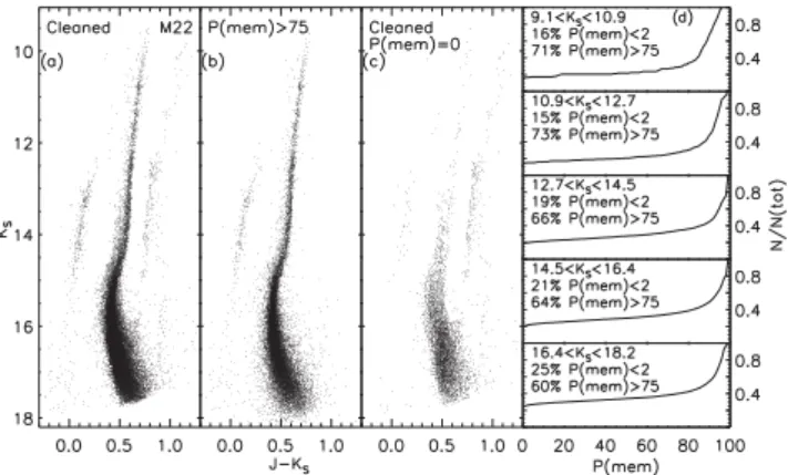
As an independent test of the decontamination procedure, we may compare our statistically decontaminated CMDs with results from relative proper motion studies. There is one cluster in our sample, M 22, for which membership probabilities have been calculated from relative proper motions over a relatively wide field of view by Libralato et al. (2014).8After matching our photometric catalogue to theirs, in Fig.3, we compare all stars in our (differential reddening-corrected) catalogue surviving statistical decontamination (shown in panel a) with those that Libralato et al. (2014) considered likely members (panel b) as well as those that survived the decontamina-tion procedure but have zero probability of membership according to their proper motions (panel c). It is evident that for this clus-ter, the decontamination procedure fails to remove a minority of field RGB stars, seen 0.2–0.3 mag redward of the cluster RGB in panels (a) and (c) of Fig.3. There are several probable causes for this effect, and proper motion selection can be similarly subject to contamination from field stars with cluster-like proper motions (e.g. Libralato et al.2015), although it may be possible to take this effect into account statistically in some cases (e.g. Milone et al.2012).
Figure 3. (a) CMD of all stars present in the proper motion catalogue of Libralato et al. (2014) that passed the statistical decontamination procedure described in Section 2.5.1. (b) All stars in our photometric catalogue that are likely proper motion members (Pmem>75) according to Libralato et al. (2014). (c) Stars that survived our statistical decontamination algorithm but have a proper motion based membership probability of 0 from Libralato et al. (2014). (d) Cumulative distribution of Libralato et al. (2014) mem-bership probability for all stars that survived the statistical decontamination procedure, shown in 5 mag bins.
To further compare the performance of the decontamination al-gorithm versus the use of proper motions as a function of magnitude (or, equivalently, photometric error), in panel (d) of Fig.3, we di-vide the stars in our catalogue that survived the decontamination algorithm into magnitude bins. In each magnitude bin, we plot the cumulative distribution of the proper motion membership probabil-ities from Libralato et al. (2014), as well as giving the fraction of surviving stars in each bin that fall into the ranges of proper mo-tion probability used by Libralato et al. (2014) to identify definite members (Pmem>75 per cent) and definite non-members (Pmem< 2 per cent). It is clear from the right-hand panel of Fig.3that the contamination rate among our statistically decontaminated sample is≤25 per cent without the use of a colour cut, and this contamina-tion rate does not vary appreciably with magnitude.
2.6 Colour–magnitude diagrams
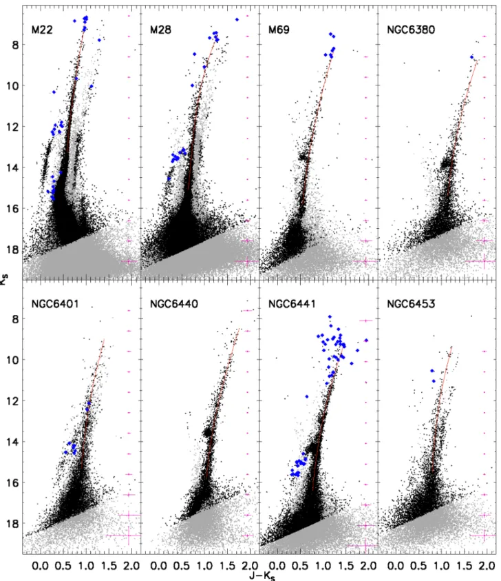
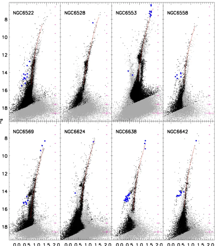
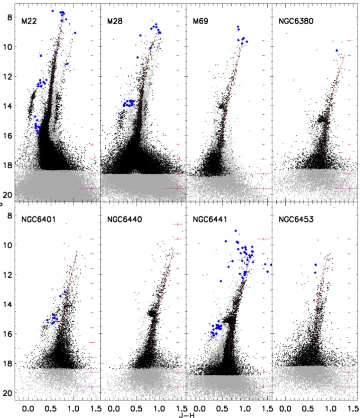
CMDs of all of our target clusters are shown in the (KS,J−KS) plane
in Fig.4and in the (J,J−H) plane in Fig.5, and are also included in the supplementary figures along with the RGB LFs. Stars that passed the decontamination procedure are shown in black, whereas stars that failed are shown in grey. In addition, we have identified known variables in our target clusters by matching our 2MASS-astrometrizedJHKScatalogues with the most recent version of the
Catalogue of Variable Stars in GGCs (Clement et al.2001)9 and the catalogue of equatorial coordinates by Samus et al. (2009). These variables are overplotted on the CMDs as blue diamonds. We have excluded known variables from the determination of the fidu-cial sequences since detailed variability studies show that asymp-totic giant branch (AGB) variables may be present faintward of the RGB tip, and a more thorough discussion of variability on the upper RGB and the inclusion of variables in RGB tip magnitude measurements can be found in Section 3.2. In any case, the influence of known variables on each of the photometric features we mea-sure is discussed in the context of each of the relevant features in Section 3.
9http://www.astro.utoronto.ca/∼cclement/read.html
While in a minority of cases, the decontamination procedure re-sults in gaps in the cluster evolutionary sequences or a failure to remove field RGB stars, this is a likely consequence of the dif-fering spatial resolution between the reddening maps applied to the comparison field (>1 arcmin; Gonzalez et al.2012) and those applied to the cluster regions before decontamination (see Alonso Garcia et al.2012; Cohen et al. 2014, Section 2.4). In addition, the fact that the clusters that are most susceptible to this effect (NGC 6553 and M22) are also the most nearby along the line of sight suggests that this could also be partially due to preferen-tial obscuration of the field (e.g. bulge) population by the clus-ter in these cases, and we note that the Gonzalez et al. (2012) map that we employ for the comparison field tends to overesti-mate reddening at small (<4 kpc) heliocentric distances (Schultheis et al.2014). In any case, we find that the location of photometric features we measure is insensitive to this effect beyond their re-ported uncertainties, based both on comparisons to previous stud-ies employing radial cuts and/or proper motions (see Section 3.5) as well as a comparison between values measured using statisti-cally decontaminated CMDs versus field-subtracted LFs (see Sec-tion 3.3.2).
3 O B S E RV E D P H OT O M E T R I C F E AT U R E S
3.1 Cluster fiducial sequences
In order to derive calibrations between cluster chemical abundances and photometric features along the cluster RGBs, including the RGB tip, bump and slope, we fit fiducial sequences to the RGBs in the differential reddening corrected, field star decomtaminated CMDs, that are hereafter referred to as the ‘processed’ CMDs. Fiducial sequences are fit using an iterative procedure similar to previous studies (Ferraro et al.2000; Valenti et al.2004a; Cohen et al.2014,2015). First, a rough visual colour–magnitude cut was used to isolate the CMD region of the RGB. Next, the RGB was divided into magnitude bins of width 0.5 mag, and the median colour and magnitude in each bin was measured. A low-order (≤3) polynomial was then fit to these median colours as a function of magnitude, iteratively rejecting stars more than 2σ in colour from the fit polynomial in each bin. This process is repeated until con-vergence is indicated by the number of surviving stars changing by under 2 per cent since the previous iteration. This procedure is still necessary even if the field star decontamination algorithm functions perfectly, since bona fide cluster HB and AGB stars should still be present and thus can be removed from considera-tion in a statistical manner to construct sequences representative of the RGB.
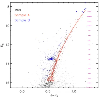
Once the fiducial sequence has been constructed, we make a colour cut in the (KS, J− KS) CMD to identify sub-samples of
stars used to measure the slope of the upper RGB as well as the locations of the red giant branch bump (RGBB) and the HB. Specif-ically, in order to minimize contamination of the cluster RGB by the HB, we use only stars with (J− KS) colours within 3σ of
the fiducial sequence (whereσrepresents the median photometric error as a function ofKSmagnitude), that we refer to as Sample
A. Similarly, to avoid a bias on the HB magnitude caused by the RGBB, we measure the location of the HB using only stars blue-ward of Sample A, that we refer to as Sample B. An example of the selection of both of these samples is shown for the case of M69 in Fig.6.
The coefficients of the fiducial sequences in both the (KS,J−KS)
Figure 4. Differential reddening corrected CMDs of all of our target clusters in the (KS,J−KS) plane. All stars within the cluster region are shown in grey,
those surviving the decontamination procedure are shown in black, and known variables that were removed from our analysis are plotted as blue diamonds. In addition, our fiducial sequences are shown in red, and median photometric errors in magnitude bins are shown along the right-hand side of each CMD in magenta. High-quality (KS,J−KS) and (J,J−H) CMDs for all target clusters are included in as a set of supplementary figures.
validity. We reiterate that these fiducial sequences are derived from photometry that has been corrected for differential reddening across the cluster relative to the cluster centre, but has not been corrected for total line-of-sight extinction.
3.2 Red giant branch tip
Figure 4 –continued
studies are similarly reliant upon 2MASS photometry at these bright magnitudes, and they likewise applied a statistical procedure to re-move field stars from 2MASS photometry. However, we redeter-mine these magnitudes for three reasons. First, application of dif-ferential reddening corrections could change these values somewhat (although this effect would likely be small due to the horizontality of the reddening vector inKS, (J−KS)). Secondly, we ensure that
all clusters (not just those in common withV10) have their TRGB
magnitudes measured self-consistently. Thirdly, we avoid luminous AGB variables unknown in previous investigations (but see below). Therefore, when identifying the location of the TRGB, we use the processed CMDs as they take the photometry in all three JHKS
bands as well as photometric errors into consideration, and select the brightest star along the cluster RGB in both theKS, (J−KS) and
Figure 5. As for Fig.4but in the (J,J−H) plane.
2MASS within theH10tidal radii as well as unmatched stars in the catalogues ofV10where available.
In many cases, selection of the brightest non-AGB cluster mem-ber is ambiguous, so the selected TRGB star is ultimately only the candidate brightest RGB star. Although a statistical uncertainty on the TRGB magnitude can be estimated based on evolutionary considerations (e.g. Ferraro et al.2000), the true uncertainty in the TRGB location may be difficult to ascertain for three reasons.
effec-Figure 5 –continued tively co-located with the TRGB in near-IR colour–magnitude and
colour–colour planes. This is illustrated in a near-IR two-colour diagram in Fig.7, where we plot AGB variables in NGC 362, NGC 2808 and M 22 from Lebzelter & Wood (2011) and Sahay, Lebzelter & Wood (2014) as diamonds. We have included only periodic vari-ables that those studies do not suspect of being non-members, and observed colours were converted to the dereddened plane usingE(B
−V) values from VandenBerg et al. (2013; or Monaco et al.2004
in the case of M22) and theRV=3.1 extinction law from appendix
B of Hendricks et al. (2012). To illustrate the coincidence of these variables with GGC RGBs, we overplot K and M giant colours from Bessell & Brett (1988) as well as predictions of 12 Gyrα -enhanced ([α/Fe]= +0.4 for [Fe/H] <0, otherwise [α/Fe]= +0.2) isochrones over a wide range of cluster metallicities (−2.5
Figure 6. The processed CMD of M69, illustrating the selection of stellar sub-samples used to measure CMD features. Sample A, used to measure the RGB slope and the RGBB magnitude, is shown in red, and Sample B, used to measure the magnitude of the HB, is shown in blue. Other symbols are as in Fig.4.
near-IR colours to∼0.03 mag (Cohen et al.2015). Additionally, dereddened colours of Mira variables towards the Galactic bulge from the surveys of Matsunaga, Fukushi & Nakada (2005) and Matsunaga et al. (2009) are shown as filled grey circles and crosses, respectively. Fig.7illustrates that variability is common close to the TRGB in the near-IR colour–colour plane as well as optical and near-IR CMDs. The problem of disentangling bright AGB and RGB cluster members is not restricted to more metal-rich GGCs, as periodic variables likely to be cluster members have also been de-tected in GGCs as metal-poor as M 15 (McDonald et al.2010), that has [Fe/H]= −2.33 (C09), in addition to the metal-intermediate to metal-poor GGCs with variables shown in Fig.7.
Thirdly, both AGB and RGB stars are often photometrically vari-able, so that even when an AGB star has a colour and/or magnitude that is separable from the RGB in the mean, it may coincide with the RGB at some pulsational phases. This is illustrated, for example, in fig. 6 of Montegriffo et al. (1995), where the location of AGB variables near the RGB tip on the CMD changes significantly as a function of their pulsational phase. However, not only do AGB and RGB stars both vary, but it is unclear whether their pulsational properties can be used to disentangle their evolutionary state. For example, the optical variability study of 47 Tuc by Lebzelter & Wood (2005) found that all cluster giants that they detected with (V−I)>1.8 are variable (see their fig. 3). Furthermore, while upper
Table 2. Coefficients of observed fiducial sequences.
(J−KS)=a0+a1KS+a2KS2+a3KS3
Cluster KS, min KS, max a0 a1 a2 a3
NGC6380 8.770 15.609 3.785 2440 −0.301 9084 0.008 4423 0.000v0000 NGC6401 9.040 15.728 3.153 7068 −0.262 6610 0.007 5405 0.000 0000 NGC6440 8.459 15.986 3.038 4719 −0.130 4930 −0.005 4349 0.000 3610 NGC6441 9.188 16.612 3.643 5592 −0.314 9566 0.008 5259 0.000 0000 NGC6453 9.402 15.720 3.190 4884 −0.293 9827 0.009 0236 0.000 0000 NGC6522 8.649 15.589 3.419 8779 −0.362 0996 0.014 7217 −0.000 1667 NGC6528 7.739 15.560 2.940 6701 −0.220 7616 0.005 1508 0.000 0000 NGC6553 6.812 15.106 2.897 0294 −0.221 6789 0.005 9164 0.000 0000 NGC6558 8.822 15.551 3.253 1687 −0.315 8048 0.009 5168 0.000 0000 NGC6569 9.192 17.227 3.095 5093 −0.248 5383 0.006 3109 0.000 0000 NGC6624 8.234 15.478 2.219 1760 −0.056 2974 −0.010 3873 0.000 4842 M28 7.548 15.314 4.923 1014 −0.837 9519 0.057 7563 −0.001 3936
M69 8.358 16.068 2.837 4305 −0.245 9917 0.006 4082 0.000 0000
NGC6638 8.682 16.256 3.185 3596 −0.287 8985 0.008 2148 0.000 0000 NGC6642 8.830 17.089 2.857 4505 −0.248 6005 0.006 9500 0.000 0000 M22 6.722 13.500 1.501 1816 −0.050 6029 −0.005 8926 0.000 3390
(J−H)=a0+a1J+a2J2+a3J3
Cluster Jmin Jmax a0 a1 a2 a3
NGC6380 10.526 17.123 3.425 0948 −0.275 5087 0.007 1731 0.000 0000 NGC6401 10.436 16.290 2.668 5162 −0.209 5136 0.005 5676 0.000 0000 NGC6440 10.214 16.779 2.193 7630 −0.047 9402 −0.005 8459 0.000 2235 NGC6441 10.532 17.612 2.382 2459 −0.092 1838 −0.004 9885 0.000 2610 NGC6453 10.622 16.802 2.481 4560 −0.204 5837 0.005 6062 0.000 0000 NGC6522 9.863 16.009 4.975 3892 −0.758 9820 0.045 5941 −0.000 9510 NGC6528 9.338 16.265 2.059 2060 −0.124 2321 0.002 2911 0.000 0000 NGC6553 8.499 15.715 2.258 5166 −0.157 3739 0.003 8187 0.000 0000 NGC6558 10.079 16.537 2.945 3618 −0.274 4620 0.007 7358 0.000 0000 NGC6569 10.471 17.562 2.152 1419 −0.092 4727 −0.003 6560 0.000 2197 NGC6624 9.536 16.365 2.352 1783 −0.185 9118 0.004 6656 0.000 0000 M28 8.825 15.205 4.499 4024 −0.711 6985 0.043 7171 −0.000 9187
M69 9.574 16.907 1.361 4957 0.051 0122 −0.014 2585 0.000 4771
NGC6638 9.936 16.999 1.788 1424 −0.070 4574 −0.002 8577 0.000 1619 NGC6642 10.023 17.402 2.295 3396 −0.185 8459 0.004 8425 0.000 0000
Figure 7. Near-IR colour–colour diagram showing dereddened colours of periodic AGB variables in several GGCs from Lebzelter & Wood (2011) and Sahay et al. (2014) as diamonds, as well as Mira variables towards the Galactic Centre from Matsunaga et al. (2005,2009) as filled grey circles and crosses respectively. K and M giant colours from Bessell & Brett (1988) are overplotted as a solid line, and predictions of 12 Gyr DSED models for [Fe/H]= −2.5 to +0.5 (increasing from left to right on the plot) as dashed lines.
RGB and AGB variables may be more easily detected owing to gen-erally larger pulsational amplitudes (Kiss & Bedding2003,2004), lower amplitude RGB stars pulsate as well, with amplitudes rang-ing from hundreths of magnitudes for the OGLE Small Amplitude Red Giants in the Magellanic Clouds (OSARGs; Soszy´nski et al. 2004) and the Galactic bar (Wray, Eyer & Paczy´nski2004) down to millimagnitudes for low-luminosity RGB stars (e.g. Bedding et al. 2010).
Disconcertingly, the success of recent variability campaigns tar-geted at luminous GGC members at both optical (e.g. Layden et al. 2010; Sahay et al.2014; Abbas et al.2015) and IR wavelengths (Matsunaga, Fukushi & Nakada2006; Sloan et al.2010) implies that the current census of variable upper RGB/AGB stars in GGCs is likely incomplete, as these stars are often saturated in photo-metric time series investigations of less luminous RR Lyrae and SX Phoenicis pulsators. Moreover, even when variability data are avail-able, it remains unclear to what extent pulsational properties aid in separating AGB from RGB members near the TRGB, especially when only a small number of time series epochs are available. On one hand, fig. 4 of Lebzelter & Wood (2005) as well as the results of Sahay et al. (2014) suggest that variability amplitude decreases with decreasing luminosity, although with a relatively small sample size and sparse time sampling, the evolutionary state of any individual case may still be unclear. Perhaps, the most useful link between pulsational properties and evolutionary state for luminous giants was illustrated using a combination of photometry and extensive time series data. To this end, Kiss & Bedding (2003,2004) found that a significant fraction of the variables below the TRGB are RGB rather than AGB stars. In addition, Soszy´nski et al. (2004) managed to efficiently separate RGB and AGB stars below the TRGB using detailed pulsational properties, revealing that RGB (e.g. non-AGB) pulsators tend to have almost exclusively short primary periods (P60 d; see their fig. 8) and small pulsational amplitudes (AI<
0.14 mag). On the other hand, Lebzelter et al. (2005) discuss the
difficulty of separating AGB and RGB stars using pulsational prop-erties. While small-amplitude variables below the TRGB appear to be dominated by RGB stars in a statistical sense, an AGB status may be difficult to exclude on any individual case-by-case basis, at least when very high-quality time series data are lacking.
The time series aspect of VVV imaging unfortunately cannot provide any clues with respect to our target cluster TRGBs, as our VVV PSF photometry saturates>1 mag below the TRGB. There-fore, given the complexities associated with choosing a single star to represent the location of the TRGB, we provide a detailed cluster-by-cluster description of our choice of TRGB star in Appendix A, and list the corresponding TRGB magnitudes in TableA1without formal uncertainties. A comparison between our TRGB magnitudes and those reported in the literature is given in Section 3.5, and we discuss empirical constraints on the precision of TRGB measure-ments in Section 4.6, and the impact of the TRGB uncertainty on RGB slope measurements in Section 4.4.1. Lastly, one possibility for definitively separating bright RGB and AGB members in the absence of high-quality time series data may be via spectroscopy (M´esz´aros, Dupree & Szalai2009).
3.3 The RGBB
The RGBB in the RGB LF was originally described by Iben (1968) and Thomas (1967), and the investigation of Fusi Pecci et al. (1990) was one of the earlier studies to quantify the relationship between the RGBB luminosity and the chemical abundances of cluster stars. Empirical relations between cluster metallicity and the RGBB lumi-nosity have been presented in optical (e.g. Nataf et al.2013) as well as near-IR (Cho & Lee2002; Valenti et al.2004b) bandpasses, and we measure the location of the bump in all threeJHKSfilters. While
we defer a discussion of the bump luminosity (and consequently of the GGC distance scale, but see Cohen et al.2015) to a forthcoming study, we demonstrate below in Section 4.5 that an accurate char-acterization of the bump apparent magnitude, in combination with other features among luminous, evolved cluster members such as the HB and TRGB, can yield distance- and reddening-independent cluster metallicities with a useful precision.
3.3.1 Measuring the bump location
To quantify the location of the RGBB in our target GGCs and its uncertainty, we construct the LF of the RGB using only stars in Sample A. In an attempt to maintain self-consistency in our analysis, the LF is built with a bin size of 0.3 mag for all target clusters, although we found that the use of bin sizes from 0.2 to 0.4 mag had a negligible effect on the resulting RGBB magnitudes compared to their uncertainties. To mitigate the effects of binning, 10 histograms are constructed per cluster, but with the bin starting points shifted fractionally each time by an increment 0.1 times the bin width, and the 10 histograms are then averaged (e.g. Gullieuszik et al.2007). The resulting LF is then fit with an exponential plus Gaussian (Nataf et al.2011,2013) as a function of apparent magnitudemin each filter:
Figure 8. An example of the observed LFs for NGC 6569 in all three JHKSfilters (left to right). In the upper panels, the LF constructed from
the processed CMDs (Sample A) is shown in black, and the exponential plus Gaussian fit obtained using equation (1) is shown in red. In the lower panels, we show the LFs constructed using Sample A, in which the LF is built using all stars in the cluster region (green), the LF of the comparison field is constructed using an identical CMD region and scaled to the spatial area of the cluster region (blue). This scaled field LF is then subtracted to yield a field-subtracted cluster LF (black), shown with the corresponding exponential plus Gaussian fit (red). In all panels, the RGBB magnitude resulting from the fits is shown as a vertical dashed line. RGB LFs, as shown for this example case, are included for all target clusters in the supplementary figures.
Figure 9. As for Fig.8, but illustrating an exponential plus double Gaussian fit due to the intrusion of the HB on the RGB LF.
There are four cases where the HB intrudes on the RGB LF due to residual small-scale differential reddening that is unaccounted for by our maps. In these cases (NGC 6440, NGC 6441, NGC 6528 and NGC 6553), the HB causes a discernible second peak in the RGB LF, so an exponential plus double Gaussian is fit (e.g. Nataf et al.2011):
An example of an exponential plus double Gaussian fit is shown in Fig.9.
Because we employ the entire magnitude range of the RGB for our exponential plus Gaussian fits rather than a restricted magnitude range around the RGBB (e.g. Nataf et al.2013; Calamida et al. 2014), the resulting RGBB magnitudes are robust to both gaps in the LFs of the processed CMDs as well as stochastic fluctuations at
the bright end of the LFs due to the exponential nature of the RGB LF.
3.3.2 Quantifying Uuncertainties
To calculate the total uncertainty on the bump magnitudes resulting from the fit, we take our multibinning approach as well as the photometric errors into account using bootstrap resampling in each cluster. For each of 1000 Monte Carlo iterations, all stars are offset in the CMD by a random amount drawn from a Gaussian distribution that has a standard deviation equal to their photometric error. The entire fitting procedure is then repeated, including the multibin generation of the LF and the exponential plus Gaussian fits, and the resulting bump magnitudes are reported for each iteration. To be conservative, the uncertainty that we report for each parameter is the quadrature sum of the reported uncertainty from the fit to the observed LF plus the standard deviation of the 1000 best-fitting values output from the bootstrapping iterations. Furthermore, if the observed value of a parameter is deviant from the median of the 1000 values output by the bootstrapping procedure by more than this standard deviation, it is considered dubious, indicated by parentheses in Table3.
To test whether the measurement of the RGBB magnitude is af-fected by discontinuities or other artefacts of imperfect field star decontamination that may be present in the processed CMDs seen in Figs4and5, we have redetermined the RGBB magnitudes us-ing an alternate procedure. Rather than constructus-ing the LF from the processed CMDs, we directly decontaminate the LF itself. A multibin LF is generated employing the stars in the CMD region occupied by Sample A, but using all stars in the cluster region before the decontamination procedure was applied. Next, another multibin LF is constructed from the same CMD area, but using only stars physically located in the comparison region (e.g. outside the cluster tidal radii). This comparison region LF is scaled to the relative area of the cluster region and subtracted from the cluster region LF, again performing 1000 Monte Carlo iterations where the comparison and cluster stars are offset by Gaussian deviates of their photometric er-rors. A comparison between the RGBB magnitudes obtained from this alternate procedure, that we refer to as Sample A, versus those obtained above from Sample A, is shown in Fig.10. The mean off-set in each filter between the RGBB magnitude from Sample A and Sample A is given in each panel of Fig.10along with the standard deviation of the mean, revealing a mean offset of<0.02 mag in all three filters. Furthermore, the uncertainties in the RGBB deter-mined using Sample A are not larger than those determined from Sample A, and the ratio of the RGBB uncertainties measured from the two samples has a median of 1 in all three filters. Given the generally smoother LFs and more stable fits to sample A as com-pared to Sample A, we adopt the RGBB magnitudes resulting from the fits to Sample A. However, both sets of RGB LFs as presented in Figs8and9are included for all target clusters in the supple-mentary figures, along with cluster CMDs zoomed on the RGBs. Finally, while a detailed study of other RGBB parameters (i.e. num-ber counts, radial gradients, and skewness) is better performed with high spatial resolution, completeness-corrected photometry, the values of the LF exponentBthat we obtain from Sample A are
B=(0.63,0.59)±(0.11,0.12) inJandKS, respectively, in
reason-able (<1σ) agreement with values found in theIband by Nataf et al. (2013).
Ta
Figure 10. The difference between the RGBB magnitudes measured using Sample A and Sample A, shown as a function ofm(RGBB) from Sample Ain all threeJHKSfilters. The grey horizontal line represents equality, and
the mean offset and its standard deviation are given at the top of each panel.
values. The magnitudes of photometric features given in Table3 are apparent magnitudes, measured using photometry that has been corrected for reddening differentially across each cluster, but has not been corrected for total line-of-sight extinction or distance.
3.4 HB magnitude
Various methods have historically been applied to measure the mag-nitude of the HB and its uncertainty, including the median of a CMD-selected region (e.g. Grocholski & Sarajedini2002; Nataf et al.2013), Gaussian fits to the LF peak (e.g. Calamida et al.2014), and the location of the maximum of the cluster LF (e.g Valenti et al. 2004a). In the IR, an obvious complicating factor is the near-verticality of the HB for less metal-rich clusters, so that an LF peak representative of the HB location is not always detectable for GGCs with exclusively blue HBs (e.g. Cohen et al.2015). Therefore, for compatibility with previous studies, we restrict our HB analysis to clusters with relatively red HBs with a detectable peak in the LF of the HB, and use the observed cluster LF peak to quantify the location of the HB inJHKSmagnitude. In order to isolate the
HB from the influence of the RGBB, we construct the LF using only stars in the processed CMDs in Sample B, that are those lying more than 3σblueward of the cluster fiducial sequences. The LF is built from this sample using the same bin sizes, multibinning, and bootstrap resampling as in the case of the RGBB. However, in lieu of a Gaussian fit to the LF, the reported HB magnitude is simply the magnitude corresponding to the LF peak. This is done both for compatibility with previous near-IR studies (e.g. Valenti et al. 2004a), and because models and data demonstrate that the HB LF may be non-Gaussian in near-IR magnitude (e.g. Salaris et al.2007, see their fig. 10). Therefore, as in Cohen et al. (2015), the reported uncertainties are the quadrature sum of the standard deviation of the LF peak over the bootstrap iterations plus the effective resolution element of the LF.
We have performed our measurement of the HB LF and its peak neglecting known RR Lyrae variables in our target clusters. To check whether their inclusion affects the measured HB magnitude, we have reperformed our fits (including the bootstrapping iterations) with all known variables included. We found that in all cases, the resul-tant HB magnitude is unaffected beyond the reported uncertainties, consistent with simulations by Milone et al. (2014) demonstrating that even in optical bandpasses, the influence of RRL photometric variability on single-epoch photometry negligibly affected the HB morphological parameters that they measured.
Figure 11. The difference between the HB magnitudes measured using Samples B and B, shown as a function ofm(HB) from Sample B in all three JHKSfilters. Symbols are as in Fig.10.
Table 4. Comparison to literature values.
Parameter This study-literature N(clus)
J(RGBB) −0.045±0.020 10
comparison analogous to Fig.10. Specifically, the HB LF was gen-erated using all stars in the CMD region occupied by Sample B before statistical decontamination, and a field HB LF was gener-ated from this same CMD area using stars spatially locgener-ated in the comparison region. The comparison region LF was scaled to the area of the cluster region and subtracted before measuring the peak of the resultant LF over 1000 bootstrapping iterations in which photometric errors were applied to both the cluster and comparison region stars. A comparison between the HB magnitudes measured from this sample, denoted as Sample B, and the HB magnitudes measured from Sample B (using the statistically decontaminated CMD directly) is shown in Fig.11. This comparison illustrates that the HB magnitudes obtained using the two methods agree to within their uncertainties, with the only slight (<1.4σ) exception of NGC 6642 in theJband, that, in any case, is excluded from the calibration of our photometric metallicity relations (see Section 4).
3.5 Comparison with literature values
We compare our observed values listed in Tables3andA1with those from the literature, using the most recent sources as follows: Where available, we use values from the systematic near-IR pho-tometric studies of our target clusters by Valenti et al. (2004a,b) andV10. Otherwise, we take from Chun et al. (2010) theKS
val-ues and RGB slope for NGC 6642, theKSmagnitude of the RGB
bump for NGC 6401 and all available near-IR parameters for M 28. Additionally, the magnitude of the RGB tip in M 22 from 2MASS is taken from Monaco et al. (2004). In Table4, we list the mean offset between our values and these literature values and its stan-dard deviation, as well as the total number of clusters available for comparison. Bearing in mind that both photometric calibration un-certainties as well as observational measurement unun-certainties con-tribute to this difference, the values are generally in good agreement. Our values for the TRGB magnitude lie∼0.1 faintward of those
re-ported by Valenti et al. (2004b), consistent with the suggestions of both Dalcanton et al. (2012) and Gorski et al. (2016) that the near-IR TRGB magnitude from the Valenti et al. (2004b) calibra-tion is 0.1–0.2 mag too bright. In this case, the discrepancy could be partially due to the exclusion of (then-unknown) AGB variables, although it is well within the margin suggested by measurement error alone: the median published uncertainty of literature TRGB measurements is 0.22 mag inKSand 0.23 mag inJandH(noting
that these reported values neglect the additional contribution from uncertainties in the photometric calibration to the 2MASS system), and we revisit empirical constraints on the precision of the near-IR TRGB magnitude in Section 4.6.
3.6 Some special cases
There are a few specific cases of clusters for which a single HB/RGBB value may not be appropriate that deserve some men-tion. For the double HBs of NGC 6440 and NGC 6569 reported by Mauro et al. (2012), the values that we obtain are in good agreement, both intermediate between the two HB peaks that they report in each cluster: for NGC 6440, we findKS(HB)=13.599±0.033, in
com-parison with their values of 13.55 and 13.67 for the two HBs, and for NGC 6569, we obtainKS(HB)=14.316±0.035 in comparison
to 14.26 and 14.35 for the two HBs. Since we employ the same data as in that study, we cannot constrain the nature of the HBs beyond the results that they report, and a more detailed study of the HB morphology in these clusters using deep, high-resolution imaging is underway (Mauro et al., in preparation). OurKS(HB) values also
agree well with those employed byM14to devise reduced CaII equivalent width–[Fe/H] relations: All clusters in common have
KS(HB) values that agree to within their uncertainties, with the
ex-ception of NGC 6638, for whichM14report a significantly brighter value (13.70±0.05 versus 14.029±0.036). This merely reflects a difference in methodology, sinceM14used the reddest part of the HB, as given by theoretical models in combination with distances ofV10, to calculate theirKS(HB) values, whereas we report the
location of the observed LF peak.
We also compare ourKS(HB) andKS(RGBB) values to those
reported for NGC 6528 by Calamida et al. (2014) using a sample of proper motion-selected cluster members. Their value ofKS(bump)
=13.85±0.05 compares well with our measurement ofKS(bump)
=13.862±0.026, and they suggest a double-peaked HB with peaks atKS=12.97±0.02 and 13.16±0.02. As we employ some of the
same data that they used, we cannot comment further on this feature, but our intermediate value ofKS(HB)=13.035±0.044 supports
both the location and atypically large width in magnitude that they report for the HB of this cluster. As they cite possible residual field contamination of their proper motion-selected sample as one possible cause of the bimodality, a detailed study of this feature may benefit from high-resolution near-IR imaging of a thoroughly cleaned sample of cluster members (Cohen et al., in preparation).
4 D I S TA N C E - A N D
R E D D E N I N G - I N D E P E N D E N T C A L I B R AT I O N S
Table 5. [Fe/H] and [M/H] values for target clusters.
Cluster [Fe/H](C09) [α/Fe] Reference [M/H] [Fe/H](M14) [Fe/H](HiRes) Reference
NGC6380a −0.40± 0.09 −0.17± 0.12 −0.72± 0.11
NGC6401 −1.01± 0.14 −0.76± 0.16 −1.10± 0.20 1
NGC6440a −0.20± 0.14 0.34 2 0.04± 0.16 −0.41± 0.11 −0.57± 0.02 2
NGC6441 −0.44± 0.07 0.21 2 −0.29± 0.10 −0.65± 0.11 −0.57± 0.02 2
NGC6453 −1.48± 0.14 −1.22± 0.16
NGC6522a −1.45± 0.08 0.35 3 −1.20± 0.11 −1.38± 0.12 −1.08± 0.13 3
NGC6528a 0.07± 0.08 0.20 4,5 0.21± 0.11 −0.24± 0.11 −0.24± 0.19 6
NGC6544 −1.47± 0.07 −1.21± 0.11 −1.50± 0.12
NGC6553 −0.16± 0.06 0.30 0.05± 0.10 −0.13± 0.11 −0.20± 0.15 7
NGC6558a −1.37± 0.14 0.37 8 −1.10± 0.16 −1.07± 0.11 −0.97± 0.15 8
NGC6569a −0.72± 0.14 0.43 9 −0.40± 0.16 −1.18± 0.11 −0.90± 0.02 9
NGC6624a −0.42± 0.07 0.37 9 −0.15± 0.11 −0.72± 0.12 −0.79± 0.02 9
M28 −1.46± 0.09 −1.20± 0.12 −1.31± 0.12
M69 −0.59± 0.07 0.31 10 −0.37± 0.10 −0.66± 0.12 −0.77± 0.02 10
NGC6638 −0.99± 0.07 −0.74± 0.11 −0.95± 0.12
NGC6642a −1.19± 0.14 −0.94± 0.16 −1.40± 0.20 1
M22 −1.70± 0.08 0.32 11 −1.47± 0.11 −1.83± 0.11 −1.75± 0.04 12
aCluster excluded from calibrations in Sections 4.4.1, 4.5 and 4.6 due to uncertain metallicity. References: (1) Minniti (1995), (2) Origlia et al. (2008),
(3) Ness et al. (2014), (4) Zoccali et al. (2004), (5) Origlia et al. (2005), (6) Sobeck et al. (2006), (7) Alves-Brito et al. (2006), (8) Barbuy et al. (2007), (9) Valenti et al. (2011), (10) Lee (2007), (11) Marino et al. (2011), (12) Mucciarelli et al. (2015).
KS, (J−KS) plane (slopeJK), as well as the magnitude difference
be-tween the HB and RGBB (mHB
RGBB) and the magnitude difference between the RGB bump and the tip of the RGB (mRGBB
TRGB) in each of the threeJHKSbandpasses. While we defer a discussion of
cal-ibrations versus absolute magnitude, and hence the GGC distance scale to a forthcoming publication, the distance- and reddening-independent relations that we derive can serve as quantitative tests of evolutionary models as well as photometric metallicity indicators for old stellar populations.
4.1 Input metallicities: [Fe/H]
We wish to use GGCs with the most reliable spectroscopic abun-dances to calibrate relations between photometric features and clus-ter metallicity. While recent large-scale spectroscopic campaigns have vastly increased the number of GGCs with high-quality self-consistent spectroscopic measurements of both [Fe/H] and [α/Fe] (C09; Carretta et al.2010; Dias et al.2016), the issue of spectro-scopic metallicities remains complicated with regard to the GGCs located towards the Galactic bulge. In some cases, the values of [Fe/H] listed byC09 are significantly at odds with those from other recent, independent spectroscopic investigations. Therefore, we summarize in Table5various spectroscopic [Fe/H] values for our target clusters from several sources in addition toC09. These include the near-IR CaIItriplet studies byM14, and an additional set comprised of any independent spectroscopic metallicity mea-surements in the literature, that we denote as ‘HiRes’. These values are further compared in Fig.12, where we plot [Fe/H] fromC09 versus the HiRes values in the top panel. Significant (>0.3 dex) discrepancies are evident, as noted byM14, who devised a set of ‘corrected’C09values (that they denote ‘C09c’) for clusters where C09 values showed significant discrepancies from other studies. In the bottom panel of Fig.12, we compareC09[Fe/H] with the values given by the Ca IItriplet calibrations of M14, employing their best-fitting relations of Ca IIequivalent width versus C09c [Fe/H] values, that are cubic in the case of the Saviane et al. (2012) equivalent widths (column IIIa of their table 3) and quadratic in the case of the Rutledge, Hesser & Stetson (1997) equivalent
Figure 12. Comparison between [Fe/H] values reported byC09, versus those from independent spectroscopic studies (top panel) as well as the CaII triplet calibration ofM14(bottom panel). Clusters included as calibrators are plotted in black, and those excluded due to controversial [Fe/H] values are plotted in grey. The dotted horizontal line in each panel represents equality, and clusters are labelled by NGC or Messier number.
widths (column IIa of their table 6). The uncertainties on theM14 [Fe/H] values employed in Table5and Fig.12are the unbiased rms that they report from the applicable calibration (evaluated considering only the calibrating clusters), and for the two clus-ters with equivalent width measurements from both Saviane et al. (2012) and Rutledge, Hesser & Stetson (1997) (NGC 6528 and NGC 6553), we use the [Fe/H] values resulting from the calibra-tion employing the more recent Saviane et al. (2012) equivalent widths.
calibrations of photometric indices versus metallicity, and we later use our results to comment on the metallicities of these clusters. The remainder of our VVV targets, plotted in black in Fig.12, are used to calibrate photometric metallicity indicators, together with recent literature results. Meanwhile, a few of the cases listed in Table5 de-serve further comment regarding their HiRes [Fe/H] values as they have been subjected to multiple recent spectroscopic investigations. NGC 6522: spectroscopic analyses were recently presented by both Ness, Asplund & Casey (2014) and Barbuy et al. (2014), targeting eight and four giants, respectively. Despite having sev-eral stars in common, the two studies report mean [Fe/H] values that differ by 0.2 dex, albeit with an uncertainty of 0.15 dex in both cases. In addition, Ness, Asplund & Casey (2014) find that the cluster is significantlyα-enhanced, while Barbuy et al. (2014) claim only low to moderate enhancements of Si, Ca and Ti. We choose to adopt the abundances of Ness et al. (2014) due to their larger sample size, but we recalculate the mean [Fe/H] exclud-ing star B-108 as Barbuy et al. (2014) found that it is blended, bringing the two studies into agreement at the 1σ level. While we cannot exclude the possibility that any of the three stars in the Ness et al. (2014) sample not studied by Barbuy et al. (2014) is likewise affected by blending, there is no obvious indication among the reported radial velocities or abundances that this is the case.
NGC 6528: as discussed byM14and Dias et al. (2016), several recent spectroscopic studies have found [Fe/H] values lower than the supersolar value of [Fe/H]=+0.07±0.08 from Carretta et al. (2001) used in the compilation ofC09. Origlia, Valenti & Rich (2005) report [Fe/H]= −0.17±0.01 from high-resolution near-IR spectra of four RGB stars, while Zoccali et al. (2004) and Sobeck et al. (2006) report [Fe/H]= −0.1±0.2 and−0.24±0.19 dex, respectively, from high-resolution optical spectra of three stars (one HB star and two RGB stars). Both of these values are in good agreement with the low-resolution optical spectra of 17 stars by Dias et al. (2015), who report [Fe/H] = −0.13± 0.05, and we adopt the estimate of Sobeck et al. (2006) for the HiRes set of [Fe/H] values and comment further on photometric constraints in Section 5.
M 22 (NGC 6656): several spectroscopic investigations have claimed a split/multimodality in [Fe/H] (Marino et al.2011,2012; Alves-Brito et al.2012; Marino, Milone & Lind2013). However, Mucciarelli et al. (2015) found that when FeIlines, that are more vulnerable to non-local thermodynamic equilibrium effects, are ex-cluded, FeIIlines show no significant spread in iron abundance. For our purposes, this turns out to be somewhat of a moot point, since the value that Mucciarelli et al. (2015) calculate from FeIIlines, [FeII/H]= −1.75±0.04, is in good agreement with theC09value of [Fe/H]= −1.70±0.08, so we include this cluster in our set of calibrators.10
4.2 The global metallicity [M/H]
Since models and observations both suggest that the upper RGB is sensitive to variations in [α/Fe] as well as [Fe/H] in the near-IR (Cohen et al.2015), we build relations in terms of both [Fe/H] and the global metallicity [M/H], defined by Salaris, Chieffi &
10Incidentally, these [Fe/H] values are not, on average, inconsistent with other high-resolution studies. Despite reporting a bimodality in [Fe/H], the spectroscopic study of 35 RGB stars by Marino et al. (2011) gives a mean value of [Fe/H]= −1.77±0.03 dex.
Straniero (1993) as [M/H] = [Fe/H] + Log(0.638fα + 0.362), wherefα =10[α/Fe]. For clusters without spectroscopic measure-ments of [α/Fe], we assume the linear [α/Fe]–[Fe/H] relation of Nataf et al. (2013), and conservatively assumeσ[α/Fe]=0.1 dex. This yields 0.3<[α/Fe]<0.4 for all target clusters without litera-ture values of [α/Fe], in accord with spectroscopic measurements of
α-enhancement found in GGCs towards the Galactic bulge (Origlia, Rich & Castro2002; Origlia et al.2005; Barbuy et al.2007; Origlia, Valenti & Rich2008; Valenti, Origlia & Rich2011; Valenti et al. 2015). In the case of NGC 6528, Zoccali et al. (2004) find [α/Fe] ∼0.1, whereas Origlia et al. (2005) report [α/Fe]∼0.33, so we assume [α/Fe]=0.2±0.1. In all cases, we calculate the uncer-tainty in the resulting [M/H] following equation 7 of Nataf et al. (2013),11and the values of [α/Fe] and their sources as well as the resulting [M/H] for our VVV target clusters are listed in Table5.
4.3 Extending the calibration baseline
Although our target clusters span a reasonably broad range in metal-licity, they suffer from the limitation that there are no GGCs included that are more metal-poor than M 22 ([Fe/H]−1.7). In order to maximize the applicable metallicity range of our calibrations as well as increase the sample size, we supplement the values that we measure with those available in the literature that have high-quality spectroscopic abundances (C09; Carretta et al.2010). For this pur-pose, we denote the target clusters described thus far as the ‘VVV’ sample (including NGC 6544, as described in Cohen et al.2014), and supplement them with near-IR measurements of 12 optically well-studied GGCs from Cohen et al. (2015; the ‘ISPI’ sample), as well as the data base of near-IR GGC photometry from V10 and references therein, designated the ‘V10’ sample.12 For con-venience, we have compiled measured photometric features from these supplementary sources in Table6.
We now describe the construction of relations between cluster metallicity versus several relative photometric indices that can be measured from cluster CMDs. The indices studied typically span a colour range of(J−KS)0.5, so in addition to being independent
of distance and reddening, they are insensitive to photometric zero-point uncertainties and the assumed reddening law.
4.4 RGB Slope (slopeJK)
4.4.1 Observed slope measurements
A linear relation has traditionally been used to describe cluster metallicity (in terms of [Fe/H] and/or [M/H]) versus the slope of the upper RGB (in terms of colour as function of magnitude), calculated over a magnitude range on the upper RGB where the effects of metallicity variations are most prominent (e.g. Valenti et al.2004a). The definition of this magnitude range is based on the observation of Kuchinski et al. (1995) that using stars in the range of 0.6–5.1 mag brighter than the zero-age horizontal branch (ZAHB) serves to avoid the influence of HB stars at the faint end and bright AGB variables close to the RGB tip. However, defining a ZAHB magnitude for metal-poor clusters in the near-IR is difficult
11Where not given explicitly, we calculateαas the mean of Ti, Si, Mg and Ca (e.g. Valenti et al.2011) weighted by the inverse squares of their uncertainties.
Figure 13. Relations between the slope of the red giant branch and cluster metallicity, in terms of [Fe/H] (top) and global metallicity [M/H] (bottom). In each plot, values for clusters from the VVV sample are shown as filled black circles. Clusters in the VVV sample that are excluded as calibrators due to uncertain metallicities are labelled and plotted in grey rather than black, and theirC09values are connected by a dotted line to values corresponding to [Fe/H] from
M14(open diamonds) and the HiRes set given in Table5(open circles). Additional clusters used as calibrators from theV10sample (V10, and references therein) are shown as blue squares, and calibrators from Cohen et al. (2015) are shown using red circles. The solid black line represents a least-squares fit to all calibrators (VVV+V10+ISPI) weighted using the uncertainties in metallicity, and the resulting best-fitting equation is given in the bottom right corner of each panel. The dashed black line represents the relation of Valenti et al. (2004a) transformed to theC09metallicity scale. The curved grey lines represent the median and±1σvalues predicted from Monte Carlo simulations using Victoria–Regina evolutionary models (see the text for details), and the individual simulation results are shown as light grey points.
since their HBs are, in fact, almost vertical, so for consistency, we follow the methodology of Valenti et al. (2004a, and references therein) and use the magnitude range of 0.5<(K−KTRGB)<5.0. The RGB slope is measured by fitting a line to all stars that lie in this magnitude range and have colours within 3σ of the fiducial sequence (e.g. included in Sample A).
In Fig.13, we show measured RGB slope values versus both [Fe/H] and [M/H] (on theC09 scale). Target clusters from the VVV sample are shown as filled black circles, while those from the literature are shown using blue squares (V04 sample) or red circles (ISPI sample). VVV clusters that were not used as calibrators due to their uncertain [Fe/H] values are shown in grey and labelled by NGC number, and for each of these clusters, a vertical dotted