FDTD-based Transcranial Magnetic Stimulation model applied to specific neurodegenerative disorders

FDTD-based Transcranial Magnetic Stimulation model

applied to specific neurodegenerative disorders

Félix Fanjul-Vélez, Irene Salas-García, Noé Ortega-Quijano, José Luis Arce-Diego

Applied Optical Techniques Group, Electronics Technology, Systems and Automation

Engineering Department, University of Cantabria, Avenida de los Castros S/N, 39005

Santander, Spain

[email protected]

;

[email protected]

Abstract

Non-invasive treatment of neurodegenerative diseases is particularly challenging in Western countries, where the population age is increasing. In this work, magnetic propagation in human head is modeled by Finite-Difference Time-Domain (FDTD) method, taking into account specific characteristics of Transcranial Magnetic Stimulation (TMS) in neurodegenerative diseases. It uses a realistic high-resolution three-dimensional human head mesh. The numerical method is applied to the analysis of magnetic radiation distribution in the brain using two realistic magnetic source models: a circular coil and a figure-8 coil commonly employed in TMS. The complete model was applied to the study of magnetic stimulation in Alzheimer and Parkinson Diseases (AD, PD). The results show the electrical field distribution when magnetic stimulation is supplied to those brain areas of specific interest for each particular disease. Thereby the current approach entails a high potential for the establishment of the current underdeveloped TMS dosimetry in its emerging application to AD and PD.

Keywords: FDTD, Transcranial Magnetic Stimulation, Circular coil, Figure-8 coil,

Alzheimer Disease, Parkinson Disease.

1. Introduction

The study of neurodegenerative processes and the development of techniques for their treatment are nowadays an area of great relevance. This is due to their enormous impact, not only from a medical point of view, but also due to their intrinsic social and economic aspects. The

increasing trend of global aging has intensified the need to find effective solutions to diseases strongly related to ageing, such as Alzheimer (AD) or Pakinson (PD) diseases [1]. Emerging therapeutics for these disorders include those that employ energy sources of different nature (electrical, magnetical, optical) to stimulate specific functional brain regions that have been altered during the neurodegeneration process [2]. Among them, Transcranial Magnetic Stimulation (TMS) is one of the most explored due to its capacity for the neuromodulation of specific neural networks with therapeutic purposes and the subsequent promising results obtained in several clinical trials with AD and PD patients [3, 4]. In the last years a growing number of studies have showed promising effects of TMS over an increasing number of pathologies. The clinical trials database by the U.S. National Institute of Health (NIH) shows a significant number of studies (both finished and currently recruiting participants) related to TMS, which is a clear indicator of the potential offered by this non-invasive treatment technique. These studies include neurodegenerative diseases which have nowadays no cure. However, despite its high potential for its future clinical implantation, some controversies related to the proper TMS dosimetry remain unsolved due to the lack of reproducibility in certain clinical trials, the complexity of neuronal activity, the great amount of factors that can affect the response to the magnetic stimulation and the lack of multi-centre trials with a larger number of patients [5]. The development of predictive models constitutes a valuable tool to establish the adequate dosimetric parameters to get a certain therapeutic benefit or to design and analyze scientific studies based on TMS experiments with both diagnostic and research purposes [6]. This requires an accurate computation of the induced electrical field within the brain as well as thedielectric properties of the brain tissues [7]. Early studies in this area were mostly based on spherical models [8], whereas the most recent ones employ a high-resolution model of human head and numerical methods such as the finite element method (FEM) [9, 10]. These last ones have allowed a precise calculus of the field induced by common TMS coils in the human head. However the previous studies, such as one of the same authors [11], have not been focused on the electrical field induced by coils precisely positioned over functional brain regions that have been identified as pinpoint targets to treat the main symptoms associated with

neurodegenerative diseases. Up to now coil positioning to deal with a specific disorder was taken into account only for depression using an impedance method [12].

We present a Finite-Difference Time-Domain (FDTD)-based TMS model, which is applied to specific dysfunctions associated with AD and PD in order to predict the electromagnetic propagation in a realistic model of adult human head. A specific FDTD method is used for modeling low-frequency magnetic propagation in a brain undergoing TMS with single and double stimulation coils positioned over functional areas of interest for both types of disorder. The results enable to observe the main characteristics of each type of stimulation. The analysis performed in this work constitutes the first approach towards the development of comprehensive predictive models that could enable to determine the magnetic radiation distribution in the brain, in order to appropriately control radiation parameters for enhancing and optimizing the stimulation process.

Section 2 describes the theoretical foundation underlying the FDTD-based TMS model, which includes a brief review of the well-known FDTD method, as well as the implementation and positioning of two types of coils commonly used in the ongoing clinical trials involving neurodegenerative diseases. In Section 3 the model previously described is particularized for magnetic propagation during TMS in AD and PD. Results in Section 4 show the electric field induced in the brain regions of interest for both diseases using a single and a double coil with variable orientation. Finally, the main conclusions are presented in Section 5.

2. Description of the electromagnetic propagation model for TMS

This section describes the theoretical foundation underlying the FDTD-based TMS model which includes a brief review of the FDTD method as well as the implementation and positioning of two types of coils commonly used in the ongoing clinical trials involving neurodegenerative diseases.

2.1 FDTD method

The FDTD method is a widely-used approach for numerically solving electromagnetic propagation through different types of media. FDTD method exhibits very high accuracy and versatility, which makes it an essential tool for electromagnetic studies in many applications. In particular, it has been demonstrated that FDTD is a robust and efficient computational method for the calculation of magnetic propagation in biological tissues [13, 14]. One example of its wide application is in [14], where FDTD was used to investigate the cerebral fields induced in a head model undergoing a different brain stimulation technique, electrical stimulation (Transcranial alternating current stimulation (tACs)). tAC directly applies current by stimulating electrodes, on the contrary of magnetic stimulation, which is applied by means of the magnetic coils employed in TMS to induce the desired cortical currents. Although at neuron level TMS excites the neurons with the same mechanism as electrical stimulation, the former is non-invasive. Previous works show that FDTD is a robust and efficient computational method for the calculation of magnetic propagation in biological tissues. However, as it is explained later in Section 3, devoted to the model application, its use for the study of magnetic propagation in human head for brain stimulation at low frequencies greatly increases the computational load. In this case, the computation problem can be solved by a frequency scaling method. In this section we present a concise description of the FDTD method, introducing the essential concepts and including all the fundamental equations involved in the process except the source model, which will be discussed in the next two subsections.

FDTD method constitutes a direct implementation of Maxwell’s equations in the time domain. This approach for solving Maxwell’s equations may present limitations in terms of accuracy. Although these limitations can be overcome by means of adequately choosing the grid parameters and the temporal step [15]. In the present work, the spatial grid was chosen so as to cope with stability conditions, taking into account the geometry of the problem and the wavelength of the electromagnetic radiation. Therefore firstly a spatial discretization is performed using a rectangular mesh of

(

N N_x, _y,N_z

)

cubes with a constant cell size

characterized by the edge length ∆ . Numerical stability conditions impose a minimum _ijk number of 20 cells per wavelength. As a consequence, the approach is valid under the stability conditions point of view. The basic element of the spatial mesh is given by the Yee lattice, in which the electromagnetic field vectors involved in the FDTD method have been depicted. Along with spatial discretization by a rectangular mesh, time is also discretized with a temporal step ∆t. Stability conditions impose a maximum time step defined by eq. (1), where c_max is the highest electromagnetic wave propagation speed in the medium.

max 2 1 3 ijk t c ∆ ≤ ∆ (1)

From Maxwell’s equations, and adapting partial derivatives to the spatial and temporal discretization described above, the equations for calculating the electric and magnetic fields for each position and time instant are obtained [13]. In particular, the magnetic field componentsHx

, H and y H (defined in the face center of each cube, whose cell identifier is denoted by the z

subscript) are obtained for the intervals between two consecutive time instants (denoted by the superscript) by the eqs. (2) to (4), where the coefficients 1

x

H and 2

x

H are respectively given by eqs. (5) and (6).

(

)

1 2 1 2 1 2 , , , , , , , , , , 1 , , , , , 1, n n n x n x n n xi j k i j k xi j k i j k yi j k y i j k zi j k zi j k H + =H H − +H E ₊ −E +E −E ₊ (2)

(

)

1 2 1 2 1 2 1, , , , , , , , 1 , , , , , , , , n _y n _y n n n n yi j k i j k yi j k i j k zi j k zi j k x i j k x i j k H + =H H − +H E ₊ −E +E −E ₊ (3)

(

)

1 2 1 2 1 2 , , , , , , , , , 1, , , , , 1, , n n n z n z n n zi j k i j k zi j k i j k xi j k x i j k yi j k y i j k H + H H − H E ₊ E E E + = + − + − (4)

(

)

(

)

1 , , , , 1 _{, ,} 1 , , , , 1 2 1 2 x x i j k i j k x i j k x x i j k i j k t H t ρ µ ρ µ − − − ∆ = + ∆ (5)

(

)

(

)

1 , , 2 _{, ,} 1 , , , , 1 2 x ijk i j k x i j k x x i j k i j k t H t µ ρ µ − − ∆ ∆ = + ∆ (6)

The remaining coefficients ( ₁y

H , ₂y

H , ₁z

H and ₂z

H ) are analogously defined. Magnetic permeability

µ

and magnetic losses ρ are defined in the cube nodes. If the medium is inhomogeneous, it is necessary to obtain the effective properties in order to ensure the continuity of the tangent field components. Therefore, the effective magnetic permeability and magnetic losses for the calculation of the field components along the x direction are calculated by eqs. (7) and (8) respectively.

, , , 1, , , 1 , 1, 1 , , 4 i j k i j k i j k i j k x i j k µ µ µ µ µ ₌ + + + + + + + (7) , , , 1, , , 1 , 1, 1 , , 4 i j k i j k i j k i j k x i j k ρ ρ ρ ρ ρ ₌ + + + + + + + (8)

The equations for the remaining directions, and those for the electric field, can be obtained in the same way [13].

Finally, it is necessary to fix the Absorbing Boundary Conditions (ABCs) in order to avoid reflections and calculation errors in the edges of the spatial mesh. There are several methods widely used for this purpose [15]. In this work, we have used Mur’s ABCs improved by the superabsorption method [16]. The first order Mur’s ABCs are given for the electric field. Specifically, in the particular case of the ABCs for the z component of the electric field in the

xy plane, the conditions imposed by the first-order Mur’s ABCs are those expressed in eq. (9) which are implemented in the FDTD method as in eq. (10).

0 min 0 max 0 , 0 , z z z z E E c z z t x E E c z z t x ∂ ∂  _{− = =}  ∂ ∂ ∂ ∂  _{+ = =}  ∂ ∂  (9)

(

)

(

)

0 1 1 1, , 2, , 2, , 1, , 0 0 1 1 1, , , , , , 1, , 0 , 1: 1, 1: , 1: 1, 1: x x x x ijk n n n n z j k z j k z j k z j k y z ijk ijk n n n n z N j k z N j k z N j k z N j k y z ijk c t E E E E j N k N c t c t E E E E j N k N c t + + + + + + ∆ − ∆  = + − = + =  _{∆ + ∆}   _{∆ − ∆}  _{= + − = + =}  _{∆ + ∆}  (10)

The equations above can be straightforwardly extended to the remaining components of the electric field with minor changes of the subscripts. Regarding the superabsorption conditions, they constitute an improvement of Mur’s ABCs in terms of robustness and accuracy. The essential aim of superabsorption conditions is to compensate inconsistencies that are present in the boundary magnetic fields components due to residual errors in the electric field components calculated by Mur’s ABCs. If we consider the y component of the magnetic field, the first step in the superabsorption method is to calculate H_y in the boundaries using the basic equations of the FDTD method, which yields H_{y1, ,}n+_{j k}1 2 1( ) and 1 2 1_{, ,}( )

x

n y N j k

H + . After that, Mur’s ABCs are applied to H_y, which gives H_{y1, ,}n+_{j k}1 2 2( ) and 1 2 2_{, ,}( )

x

n y N j k

H + . Subsequently, the final value of H_y in the boundaries is given by eq. (11).

( ) ( ) ( ) ( ) 1 2 1 0 1 2 2 1, , 1, , 1 2 1, , 0 1 2 1 0 1 2 2 , , , , 1 2 , , 0 , 1: 1, 1: 1 , 1: 1, 1: 1 x x x n n y j k y j k ijk n y j k y z ijk n n y N j k y N j k ijk n y N j k y z ijk c t H H H j N k N c t c t H H H j N k N c t + + + + + + ∆  ₊  _∆  _{= = + =} ∆  ₊  _∆   _∆  ₊  ∆ = = + =  _∆  ₊  ∆  (11)

2.2 Coil model

This section describes the modeling of two magnetic sources (i.e. circular-shaped and figure-8 coils) commonly used in TMS that were used in the previous FDTD method.

2.2.1 Circular coil

In this Section, we summarize a method for modeling a circular coil as an ensemble of simple dipoles. It has been shown that the electromagnetic field induced by a circular coil can be modeled by the superposition of the fields produced by several dipoles located at specific positions [17]. In particular, the approach firstly requires dividing the coil area into subregions, and subsequently locating a dipole in the center of each of them. In that way, the normal

component of the magnetic field (denoted as B r

(

,β

)

in two dimensional polar coordinates, where r is the radius and β the angle) is approximated by the weighted sum in eq. (12).

(

)

(

)

2 1 0 0 , , b r _N k k k k B r r dr d p B r π β β β = ⋅ ⋅ =

∑

∫ ∫

(12)

In eq. (12)

N

is the number of dipoles,

p

_k is the weight associated with each of them and

(

_k

,

_k

)

B r

β

is the magnetic field for each dipole located at the corresponding polar coordinates. The determination of the weight and the position associated with each dipole is carried out by numerical solving of systems of nonlinear equations [18]. Here we consider the modeling of a circular coil by 12 magnetic dipoles, as shown in Figure 1a). This model has a satisfactory degree of accuracy for coils to within approximately 60-80 mm, depending on several spatial parameters [8]. In this case, the parameters employed are listed in Table 1.

Figure 1. a) Circular coil model with 12 magnetic dipoles (the position and the weight associated to each dipole are included in Table 1) b) Figure-8 coil modelling by means of 24 dipoles.

Table 1. Parameters that determine the position and the weight associated to each of the 12 dipoles employed to model a circular shaped coil of radius r_b [18].

Angle (

β

k

)

Radius (

r

k

)

Weight (

p

k

)

Dipole number

1 2 2 k

π

 ₋     

0.45667

⋅

r

b 2 0.12321⋅

π

r_b

k

=

1...4

2 k

π

0.86603

⋅

r

_b 2 0.074074⋅

π

rb

k

=

5...8

1 2 2 k

π

 ₋     

0.91100

⋅

r

b 2 0.052715⋅

π

r_b

k

=

9...12

Each magnetic dipole can be modeled using a small-sized coil without magnetic core comprising a coil with a cross section A and

N

turns whose magnetic moment is expressed in eq. (13), where

i t

( )

is the current pulse that excites the coil.

( )

( )

z

M t =ANi t (13)

Here we use Gaussian pulses as described by the eq. (14).

( )

0

(

0

)

2 0 exp ₂ 2 s t t t t i t I τ τ  ₋  − = −      (14)

The parameter

τ

determines the center frequency of the pulse, given by

f

_c

=

0.16

τ

, and the 3 dB bandwidth, that is

BW

=

1.15

f

_c. FDTD simulations were carried out at 1 MHz, using the dielectric parameters for the brain layers at the desired frequency and applying a posterior scaling method to the results [13].

The initial position of the dipoles that model the coil is in the plane yz located in the right side of the head. Afterwards they are rotated in the space by the method described below.

The position of each dipole in the yz plane specified in the reference system x0_y0_z0 _{can be}

expressed by means of eq. (15) to (17). Where

r

_k y

β

_k are the radius and the angle for the k-dipole respectively, whose values were reported in Table 1.

0 k b x =s (15)

( )

0 _cos k k k y =r β (16)

( )

0 sin k k k z =r β (17)

The implementation of each magnetic dipole in the FDTD method is performed by the double-closed current loop model [19]. According to this method, the total current density for each of the two loops that model the magnetic moment of the dipole can be expressed as in eq. (18).

( )

4

( )

2 s ijk AN J t = i t ∆ (18)

In this case, the current density should be weighted by the weight associated to each dipole according to the values in Table 1 and the expression (19). So the moment of the magnetic dipole can be approximated by the weighted sum shown in eq. (20) in an analogous way to the magnetic field.

( )

( )

s _k k s J t = p J t (19)

( )

( )

1 N s k s k J t p J t = =

∑

(20)

2.2.2 Figure-8 coil

This section addresses the model of a figure-8 coil from the extension of the circular coil model previously described. In this case a figure-8 coil can be modelled by means of 24 dipoles (12 for each of the two circular coils that comprise it) as it is depicted in Figure 1b). Taking into account the structure of the figure-8 coil, two new parameters should be considered: the margin between the coils (m), which fixes the spacing between them, and the orientation of the coil axis (ψ).

As in the case of the circular coil, the position of the dipoles is initially specified in the yz plane of the head reference system. In this case, the position of the 12 dipoles that model the first circular coil shape is given by eq. (21) to (23).

0 k b x =s (21)

( )

( )

0 _cos 1 _cos 2 k k k b y =r β +_r + m_ ψ   (22)

( )

( )

0 _sin 1 _sin 2 k k k b z =r β +_r + m_ ψ   (23)

The position of the remaining 12 dipoles for the second circular coil can be determined by the eq. (24) to 263). 0 k b x =s (24)

( )

( )

0 1 cos cos 2 k k k b y =r β −_r + m_ ψ   (25)

( )

( )

0 1 sin sin 2 k k k b z =r β −_r + m_ ψ   (26)

Finally, the current density is set to opposite sign for the two circular coils as it is expressed in eq. (27).

( )

_1...12

( )

_13...24

s _k s _k

J t ₌ = −J t ₌ (27)

The rest of parameters involved are the same that those used in the modelling of a simple coil, therefore the weight and the position of each individual dipole is obtained once again from the values listed in Table 1.

2.2.3 Coil positioning

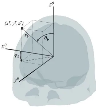
This section describes the method used to place the coil at any point in the space and therefore to apply the magnetic radiation in the required position and at the desired distance of the head. For this purpose it is necessary to set the reference system. First the head reference system x0_y0_z0 _{whose origin matches the center of the brain mesh is defined as it is shown in Figure 2.}

Figure 2. Source position in the head reference system x0_y0_z0 _{expressed by means of polar}

coordinates {θb, φb, sb} and Talairach coordinates {xT, yT, zT}.

According to this scheme, the central position of the source can be uniquely defined in spherical coordinates in this reference system by means of three parameters: the polar angle

θ

_b, the azimuthal angle

ϕ

_b and the radius

s

_b. The Talairach coordinates {xT_{, y}T_{, z}T_{} of the source are}

directly related to the spherical coordinates by means of eq. (28) to (30).

( ) ( )

sin cos T b b b x =s θ ϕ (28)

( ) ( )

sin sin T b b b y =s θ ϕ (29)

( )

cos T b b z =s θ (30)

The three coordinates define the position vector s_k0 expressed in eq. (31).

0 0 0 k k k x y z     =       0 k s  (31)

Once we know each dipole position, it is necessary to rotate the position vectors to place them at the final position specified by the polar angle

θ

_b and the azimuthal angle

ϕ

_b. Such

three-dimensional rotation can be carried out by means of two consecutive rotations. First, a rotation over the axis y0 is described by the matrix in eq. (32), where the rotation angle

α

_y is directly related to the polar angle according to eq. (33).

( )

( )

( )

( )

cos 0 sin 0 1 0 sin 0 cos y y y y α α α α     =   ₋    y R (32) 2 y b π α = −_ −θ _   (33)

The second rotation is implemented over the axis z0 as it is described by eq. (34) where the rotation angle

α

_z is exactly the same as the defined azimuthal angle (α_z=ϕ_b).

( )

( )

( )

( )

cos sin 0 sin cos 0 0 0 1 z z z z α α α α  −    =       z R (34)

The concatenation of these two rotation operations over the initial position vector s_k0 in the yz plane results in the position vector for each dipole in the source spatial position as expressed in eq. (35). ′ = 0 k z y k s R R s   (35) Finally, it is necessary to pass from the head reference system to the global coordinate system xyz. The position of the reference system origin x0_y0_z0 _{is known as it is determined by the}

vector

s



_c. In the specific three-dimensional mesh of adult human head employed, the vector

s



_c

is in eq. (36). 90.77 110.37 86.94     =     c s  (36)

The position

s



_k of each dipole in the global reference system is given by eq. (37). ′ = + k k c s s s    (37)

The method described provides the positions of the dipoles that model a source located at any desired point in space. The orientation of these dipoles is orthogonal to the coil plane and characterized by the unit vector n defined in eq. (38), where

n



₀ is given by eq. (39).

0 0 = n n n    (38) 0 T T T x y z     = −       n (39)

3. Application to clinical cases of Alzheimer and Parkinson undergoing

TMS

This section is devoted to the application of the model previously described to specific cases of Alzheimer and Parkinson disease subjected to TMS. Thus the selection of the parameters employed was obtained from the analysis of TMS clinical trials that have released beneficial effects over some dysfunctions associated with both neurodegenerative diseases. The parameters employed for the model of TMS in AD were obtained from [20], due to the fact that the authors observed an improvement in language dysfunction (auditory sentence comprehension) when they applied the magnetic stimulation over the left dorsolateral prefrontal cortex (DLPFC) in AD patients. Following their clinical setup, the magnetic stimulation in our model is applied over the Broadman area 8/9 with a Magstim double 70 mm coil. We have also modeled a single coil in order to assess possible differences between both types of magnetic source.

Regarding the modeling of TMS in PD, the parameters selection was carried out taking into account the clinical trial in [21], where the magnetic stimulation over the supplementary motor area (SMA) provided a relief of motor symptoms in PD patients. Therefore the magnetic stimulation in our model is applied over the Broadman area 6 with a double 70 mm coil and a

single 70 mm coil. Furthermore in the case of the single coil, two different coil orientations (ψ = 0º and ψ = 90º) were tested.

The FDTD method directly solves Maxwell’s equations in the time domain. As a consequence, it is valid for arbitrary electromagnetic radiation. However, its application for the study of magnetic propagation in human head for brain stimulation at low frequency imposes some difficulties. The fact that the frequencies commonly used in TMS are very low (roughly between 0.1 Hz and 10 KHz, although the range is commonly restricted to 0.1-100 Hz) makes it computationally unfeasible to perform a direct implementation of the FDTD method. In such situations, the problem can be solved by a frequency scaling method [13]. This method takes advantage of the quasi-static nature of the modeled situation. In particular, it is valid when the modeled volume is at least 10 times lower than the wavelength, and σ ωε+i >>ωε₀. Both conditions are verified for the case of brain tissue. According to such approach, the FDTD can be performed at a frequency f' higher than the frequency of interest f , and subsequently perform the following scaling operation:

( )

'

( )

' ' f E f E f f = . (40)

The dielectric properties included in the FDTD method are specified at frequency f . As well as that, modeling of low-frequency magnetic propagation in the human body converges in far less than a complete cycle, due to the small size of the modeled volume when compared to the wavelength. Taking into account this aspect can significantly reduce the computing time. It has been demonstrated that such approximation gives correct results for ratios of up to 1:200000. In this work 100 Hz stimulation was used due to the fact that it requires less computational load than lower frequencies providing similar results. These approximations are taken into account in our FDTD code. The method uses a three-dimensional realistic head mesh publicly available (namely Colin27 adult brain atlas FEM mesh Version 2) [22]. The total simulation volume is 212 x 240 x 208 mm. Dielectric properties of the brain layers (skull, cerebrospinal fluid, grey

matter and white matter) for the frequency considered in the FDTD simulations (100 Hz) have been taken from the available literature [23], and are listed in Table 2.

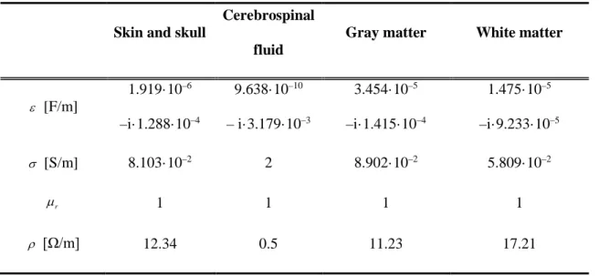
Table 2. Properties of the brain layers (100 Hz) considered in the FDTD simulations.

Skin and skull

Cerebrospinal fluid

Gray matter White matter

ε [F/m] 1.919·10–6 –i·1.288·10–4 9.638·10–10 – i·3.179·10–3 3.454·10–5 –i·1.415·10–4 1.475·10–5 –i·9.233·10–5 σ [S/m] 8.103·10–2 _{2 8.902·10}–2 _5.809·10–2 r µ 1 1 1 1 ρ [Ω/m] 12.34 0.5 11.23 17.21

4. Results and discussion

The electric field distribution was obtained taking into account the TMS setup employed in clinical trials involving AD and PD patients with beneficial effects over characteristic alterations associated with the specific pathology. Thus the parameters employed in the model were chosen taking into account the geometry and position of the magnetic source over the functional brain regions of interest for both types of disorders as it was previously expressed. Figure 3 compares the electric field distribution in the cortex of an AD patient undergoing TMS applied over the Broadmann area 8/9 (top left is the lateral view and top right is the medial view) with a single 70 mm coil and a double 70 mm coil (bottom left and right respectively). For both of them, the coil position in Talairach coordinates is

{

_xT,_yT,_zT

}

=

{

0,82.54, 47.65 mm

}

_and

{

_{, ,}

}

{

_{60 ,90 ,95.31 mm}

}

b b sb

θ ϕ =  

in spherical coordinates and its orientation is ψ = 0º. As it can be observed, both types of coil provide a clear confinement of the magnetic radiation in the desired cortex region to treat the language dysfunction associated with AD. As a consequence, possible secondary effects derived of an

inaccurate confinement are avoided. The representation of the electric field distribution under the same scale for both coils allows us to observe an increment in the field intensity when the double coil is employed. These results prove the high potential of this last type of coil for providing a better treatment directivity.

Figure 3. Region of interest: Broadmann area 8/9 (top; lateral (left) and medial (right) view). Electric field distribution normalized by its maximum value in the AD cortex undergoing 100 Hz TMS with a single 70

mm coil (bottom left) and a double 70 mm coil (bottom right).

Figures 4 and 5 show the results obtained from TMS modeling in PD. In both cases the region of interest is the Broadmann area 6 highlighted in the upper graph of Figure 4. In this last figure, the lower graphs represent a transverse view of the stimulated cortex from the top of the head with a single 70 mm coil and a double 70 mm coil (left and right respectively). In both cases the coil orientation was ψ = 0º and the Talairach coordinates of the magnetic source were

{

xT,y zT, T

}

=

{

0,50.87,72.65 mm

}

. Once again, both types of coil provide a clear confinement of the magnetic radiation in the desired cortex region, the supplementary motor area (SMA), involved in the motor symptoms of PD patients.

Finally, the double coil orientation was modified in order to assess the coil orientation influence on the electric field distribution. The results obtained are shown in Figure 5, where the graph on the left corresponds to the electric field distribution with a coil orientation of ψ = 0º and the graph on the right to an orientation of ψ = 90º. In this last case the Talairach coordinates of the

magnetic source were

{

xT,y zT, T

}

=

{

0, 43.79,75.85 mm

}

. Comparing both results a directivity dependence with the coil orientation can be clearly appreciated. Taking into account these results, the double coil oriented ψ = 0º would provide higher treatment directivity. As a consequence, better limitation of the therapeutic effects over those brain areas related to the motor symptoms associated with PD would be obtained.

Figure 4. Region of interest: Broadmann area 6 (top; lateral (left) and medial (right) view). Electric field distribution normalized by its maximum value in the PD cortex undergoing 100 Hz TMS with a single 70

mm coil (bottom left) and a double 70 mm coil (bottom right).

Figure 5. Electric field distribution normalized by its maximum value in the PD cortex undergoing 100 Hz TMS with a double 70 mm coil with different orientation (ψ = 0º on the left and ψ = 90º on the right).

The significance of the induced electric field distribution has a direct relationship with the development of an accurate treatment dosimetry that allows to determine the proper position and orientation of the magnetic source to induce the electrical current that depolarizes the desired cortical axons and triggers action potentials in the functional brain areas suitable for treating a specific pathology. As stated before, the exact relationship between the induced magnetic field and the therapeutic effect remains unclear. Although the tissue–field interaction at neuron level remains without being completely understood, the total electric field is commonly considered as the determining quantity to induce depolarization of the neuron membrane to initiate the excitation effects. Therefore the electric field distribution obtained in this work or the proportional current density is commonly employed in modeling studies as the main parameter to predict the area of stimulation. Specific brain areas are identified as targets for the treatment of several pathologies. As a consequence, the analysis made in the manuscript exploits the actual knowledge about magnetic stimulation effects to provide a tool for treatment planning. And therefore, according to these results, the application of the current TMS model presents a great interest in order to estimate the optimal magnetic source configuration to deal with specific symptoms that are characteristic of a particular neurodegenerative disease. Therefore it constitutes a first approach for the future development of predictive clinical tools able to plan the optimal TMS dosimetry for each individual patient.

Unfortunately, although an adequate treatment planning requires an a priori knowledge of the field distribution in the brain, magnetic field distribution inside the brain, or inside any other tissue, is quite difficult to measure. As a consequence, the approaches employed rely on numerical models of electromagnetic radiation. In this work, we also followed this approach. In order to assure the accuracy of the results, we employed a well-known widely used FDTD approach. The approaches for coil modeling or frequency scaling were also previously employed in other applications. Comparing the results with other studies is difficult, as we are dealing with novel complex treatment strategies that are not usually considered in full. The high

variability in the TMS setups, the patient variability and the use of unsuitable quantification metrics impede nowadays an accurate comparison with reproducible clinical results. The quantitative comparison with other published results, even with those that use a different numerical method, is also limited due to the great amount of factors that introduce variability in the final result. The qualitative analysis of the results obtained meets well known aspects, such as the high confinement of the electrical field with TMS coils. A strict verification of results obtained would entail the measurement of the electric field distribution in a significant set of subjects, knowing for each particular subject both the electromagnetic and morphological brain tissue properties. However, as far as we know, TMS modeling until the date has only provided valuable insights into the location and spatial distribution of TMS stimulation, without a sufficiently proved clinically contrasted quantification of both the stimulation and activation areas. As a consequence, the validity of the well-known FDTD approach used in the model proposed and the consistency of the results obtained with the current data available contribute to the development of predictive clinical tools able to plan the optimal TMS dosimetry.

5. Conclusions

In this work, the FDTD method has been applied to a three-dimensional realistic adult head mesh for modeling the magnetic propagation in a human brain undergoing TMS. TMS was applied to functional brain areas associated with the language dysfunction in AD and with the motor symptoms in PD. The results show that the developed tool is able to predict the radiation distribution in the brain with high resolution for different magnetic source configurations. As a consequence the model outlined provides a valuable tool for the future identification of an accurate TMS dosimetry that facilitates an adequate therapy planning, taking into account the numerous factors that may affect the final treatment response.

Conflict of interest

There is not conflict of interest.

This work has been carried out with the support of San Cándido Foundation.

References

[1] European Technology Platform Photonics 21, Photonics 21 Strategic Research Agenda (2010).

[2] S. Groppa, A. Oliviero, A. Eisen, A. Quartarone, L. G. Cohen, V. Mall, A. Kaelin-Lang, T. Mima, S. Rossi, G. W. Thickbroom, P. M. Rossini, U. Ziemann, J. Valls-Solé, H. R. Siebner, A practical guide to diagnostic transcranial magnetic stimulation: Report of an IFCN committee, Clinical Neurophysiology 123 (2012) 858–882.

[3] A. D. Wu, F. Fregni, D. K. Simon, C. Deblieck, A. Pascual-Leone, Noninvasive Brain Stimulation for Parkinson’s Disease and Dystonia, Neurotherapeutics: The Journal of the American Society for Experimental NeuroTherapeutics 5 (2008) 345–361.

[4] J. Bentwich, E. Dobronevsky, S. Aichenbaum, R. Shorer, R. Peretz, M. Khaigrekht, R. G. Marton, J. M. Rabey, Beneficial effect of repetitive transcranial magnetic stimulation combined with cognitive training for the treatment of Alzheimer’s disease: a proof of concept study, J Neural Transm 118 (2011) 463–471.

[5] R. Schulz, C. Gerloff, F. C. Hummel, Non-invasive brain stimulation in neurological diseases,Neuropharmacology 64 (2013) 579-587.

[6] D. Giordano, I. Kavasidis, C. Spampinato, R. Bella, G. Pennisi, M. Pennisi, An integrated computer-controlled system for assisting researchers in cortical excitability studies by using transcranial magnetic stimulation, Computer Methods and Programs in Biomedicine 107 (2012) 4-15.

[7] Salman Shahid, Peng Wen, Tony Ahfock, Numerical investigation of white matter anisotropic conductivity in defining current distribution under tDCS, Computer Methods and Programs in Biomedicine 109 (2013) 48-64.

[8] P. Ravazzani, J. Ruohonen, F. Grandori, G. Tognola, Magnetic stimulation of the nervous system: Induced electric field in unbounded, semi-infinite, spherical, and cylindrical media, Annuals of Biomedical Engineering 24 (1996) 606–616.

[9] A. Opitz, M. Windhoff, R. M. Heidemann, R. Turner, A. Thielscher, How the brain tissue shapes the electric field induced by transcranial magnetic stimulation, NeuroImage 58 (2011) 849–859.

[10] D. J. Bijsterbosch, A. T. Barker, K. H. Lee, P. W. R. Woodruff, Where does transcranial magnetic stimulation (TMS) stimulate? Modelling of induced field maps for some common cortical and cerebellar targets, Med Biol Eng Comput 50 (2012) 671–681.

[11] N. Ortega-Quijano, F. Fanjul-Vélez, I. Salas-García, J. L. Arce-Diego, Comparative Numerical Analysis of Magnetic and Optical Radiation Propagation in Adult Human Head, Proc. of OSA-SPIE 8803 (2013) 8803081-10.

[12] M. Nadeem, T. Thorlin, O. P. Gandhi, M. Persson, Computation of Electric and Magnetic Stimulation in Human Head Using the 3-D Impedance Method, IEEE Transactions on Biomedical Engineering 50 (2003) 900-907.

[13] C. M. Furse, Application of the Finite-Difference Time-Domain method to bioelectromagnetic simulations, Applied Computational Electromagnetics Society Newsletter (1997).

[14] Z. Manoli, N. Grossman, T. Samaras, Theoretical investigation of transcranial alternating current stimulation using realistic head model, Annual International Conference of the IEEE Engineering in Medicine and Biology Society (2012), 4156-4159.

[15] A. Taflove, S. Hagness, Computational Electrodynamics: The Finite Difference Time Domain Method, Artech House, 2000.

[16] K. K. Mei, J. Fang, Superabsorption – a method to improve absorbing boundary conditions, IEEE Trans. Antennas and Propagation 40 (1992) 1001- 1010.

[17] A. Thielschera, T. Kammer, Electric field properties of two commercial figure-8 coils in TMS: calculation of focality and efficiency, Clinical Neurophysiology 115 (2004) 1697– 1708.

[18] B. J. Roth, S. Sato, Accurate and efficient formulas for averaging the magnetic field over a circular coil, in Biomagnetism: Clinical aspects, Elsevier, 1992, pp. 797–800.

[19] R. Pontalti, J. Nadobny, P. Wust, A. Vaccari, D. Sullivan, Investigation of static and quasi-static fields inherent to the pulsed FDTD method, IEEE Trans. Microwave Theory Techniques 50 (2002) 2022–2025.

[20] M. Cotelli, M. Calabria, R. Manenti, S. Rosini, O. Zanetti, S. F. Cappa, C. Miniussi, Improved language performance in Alzheimer disease following brain stimulation, J. Neurol. Neurosurg. Psychiatry 82 (2011) 794-797.

[21] M. Hamada, Y. Ugawa, S. Tsuji, High-frequency rTMS over the supplementary motor area improves bradykinesia in Parkinson's disease: Subanalysis of double-blind sham-controlled study, Journal of the Neurological Sciences 287 (2009) 143–146.

[22] Q. Fang, Mesh-based Monte Carlo method using fast ray-tracing in Plucker coordinates, Biomed. Opt. Express 1 (2010) 165–175.

[23] S. Gabriel, R. W. Lau, C. Gabriel, The dielectric properties of biological tissues: II. Measurements in the frequency range 10 Hz to 20 GHz, Phys. Med. Biol. 41 (1996) 2251– 2269.