BiGlobal and point vortex methods for the instability analysis of wakes

BiGlobal and Point Vortex Methods for t h e Instability

Analysis of Wakes

Juan A. Tendero*"'" and Pedro Paredes"*"

School of Aeronautics, Universidad Politécnica de Madrid, Madrid, 28040, Spain

Miquel Roura*

Gamesa Innovation and Technology S.L., Madrid, 28043, Spain.

Rama Govindarajan^

TIFR Centre for Interdisciplinary Sciences, Hyderahad, 500075, India

Vassilios Theofilis^

School of Aeronautics, Universidad Politécnica de Madrid, Madrid, 28040, Spain

To b e t t e r understand destruction mechanisms of wake-vortices behind aircraft, t h e point vortex m e t h o d for stability (inviscid) used by Crow is here compared with vis-cous modal global stability analysis of t h e linearized Navier-Stokes equations acting on a two-dimensional basic flow, i.e. BiGlobal stability analysis.

T h e fact t h a t t h e BiGlobal m e t h o d is viscous, and uses a flnite área vortex model, gives rise to results s o m e w h a t different from t h e point vortex model. It adds more parameters to t h e problem, but is more realistic.

I. Introduction

T

HE problem of aircraft wakes and how long t h e y last before some mechanism destroys t h e m has been widely studied. T h e i m p o r t a n c e of t h e problem aróse a long time ago, with t h e appearance of t h e Boeing 747, and was again of importance when Airbus 380 carne into service. However, in t h e present days, not only t h e hazard due t o such big aircraft is i m p o r t a n t , also, as t h e air trafñc increases, t h e air space becomes more and more s a t u r a t e d and it is of major i m p o r t a n c e t o reduce t h e distances between aircraft t o be able t o increase t h e density of t h e m in s a t u r a t e d air spaces.

Consequently, t h e acceleration of t h e destruction of wake vórtices, although studied for a long time, is still an open problem. In t h e way t o eliminate t h a t hazard, t h e stability of t h e wake needs t o be studied in d e p t h as a previous stage, t o be able t o distinguish which configurations can last for longer and t o u n d e r s t a n d t h e mechanism of its destruction.

Here, two different methods are compared for the study of wake instabilities, the inviscid point vortex method for stability and the viscous modal stability analysis of the linearized Navier-Stokes equations using a basic flow in 2D (BiGlobal).

The first of them, which will be called inviscid, has two variants. One, applied to wakes by Kármán3'4 is a 2D analysis where the vórtices are seen as points in a plañe. The other, that involves many works, like Crow, Jiménez, Crouch and Fabre et al. amongst others, is a 3D analysis where the vórtices are seen as parallel filaments, initially straight and later with a sinusoidal perturbation.

The second method, much more modern in time, but maybe even more used, is viscous. There have been many successful ways to employ that method, but they encountered at least some difficulties, most of them involving the need of too much computational resources. Some works as Hein and Theofilis7 and Rodríguez and Theofilis have used Chebyshev-Gauss-Lobatto points, that provide high accuracy, but use a great amount of machine memory, specially when high number of grid points is needed, leading to the need of the use of big machine stations. This methods do not allow a great benefit when sparse algebra solvers are implemented, as the collocation matrices are dense and the complete matrices to solve do not have as much zeros as finite differences or other methods that do not imply full collocation matrices. Broadhurst et al. solved the problem using spectral/hp-element methods and González et al. used low order finite elements, which achieve good solutions but needed very complicated meshes. This time high order finite differences are used following the methodology of Paredes el al., which allows to obtain similar results with much less computational resources, because the use of high accuracy methods is possible for sparse matrices and then sparse algebra solvers can be implemented.

This work has been structured as follows: This first chapter is an introduction, followed by the second chapter that explains the theory behind both methods, the third chapter shows and comments the results obtained and finally some conclusions are presented in the last chapter.

II. Theory

The theory behind both inviscid vortex methods for stability analysis and viscous global modal analysis is presented in this chapter. The two methods expose some similarities, because both of them are based on the linearization of perturbed equations and the solution of an eigenvalue problem, but as the vortex methods are inviscid and based on the Biot-Savart equation, the standard analysis is a viscous method that is based on the Navier-Stokes equations. This difference in the equations leads to a difference in the variables, as these used in the vortex methods are the point or filament positions, while these of the viscous methods are the flow variables.

In addition to that, it should be noted that the Navier-Stokes are the equations that the flow follows, while the Biot-Savart relation applied to points or filaments with vorticity is only an idealization that will give good results only when the assumptions taken are valid. However, the solution of the Navier-Stokes, even linearized, gives more trouble, specially when Re is high, in other words, when viscosity is less important. That is a reason to think that inviscid methods could be a good solution, and in fact are, as it has been proved along the history. Furthermore, inviscid methods use to require less computational resources and therefore, solutions are easier to obtain in most of the cases. However, it should be noted that this inviscid limit is not the same that the solution of the Navier-Stokes equations as Re —> oo, because the highest derivative cannot go to zero. For that reason, one should never forget that inviscid methods solve an approximation which may have singularities in boundary layers and concéntrate vórtices, as well as turbulent mechanisms are neglected.

II.A. Point Vortex Linear Modal Analysis

This method for stability assumes a given set of point vórtices in a 2D plañe that are in equilibrium. However, this assumption can be relaxed to a set of points that maintain their relative positions, as it occurs for the two counter-rotative vórtices. Later a small perturbation is introduced and the equations of the movement linearized to first order in the perturbations. These linearized equations are not solved in time in this approach, instead, the temporal behavior is supposed to be in exponential form and, using this assumption, an eigenvalue problem is solved to analyze the stability of the problem.

This methodology, is similar to that used in standard global modal analysis, but here the equations of the movement are the equations that give the movement of the point vórtices and the perturbed variables are the point positions, opposed to the Navier-Stokes equations and the flow variables that are used there.

The analysis mentioned is presented for 2D point vórtices and perturbations, and later for the filaments in 3D that represent a set of points in 2D, but for sinusoidal perturbations in the third direction. This method in 3D was used by Crow to discover the wake instability that has now his ñame.

II. A.1. Two Dimensional Perturbations Procedure, particularized for two counter-rotative vórtices

The starting point is a configuration of N point vórtices in a plañe, xp = [xp,yp], each of them denoted by

the subindex p. This set of points will move following Eq. (1), where ez is the vector perpendicular to the plañe.

i N ( \

( p)~ ^ 2 - L« | xp-X g| 2 W

Perturbations of the form of xp = Xp + ex'p are introduced in the vortex positions, and later the

resulting equations are linearized, leaving only terms of order e. In order to do that, up = [up,vp] =

(híp/dt = u(xp) — Ü, where Ü is in this case the descent speed of the pair. Note that Xp represent an equilibrium configuration, and therefore, the order one part of the equation is satisfied and gives the valué of Ü = — (Ta/4irXa)ez and the order e part of the equation remain unchanged. Time derivatives are supposed

homogeneous as x'j, = ~kpe~iut. N = 2 is substituted for the case of two counter rotative vórtices. Here,

2Xa is the distance between the vórtices and ra the circulation of the right vortex, being the opposite for the left.

. , T0 (yi -y2\

~

lüJXl

= Y [W^J

(2a)

. „ rn (xi -x2\ , .

. , ro fy2 -yi\ , ,

~

1UJX2

= -^ \ w ^ )

(2c)

. , rn fx2 - ¿ i \ , .

~

1UJy2

= ~2¿ {W^J

(2d)

It is time to non-dimensionalize these equations. The distance between the vórtices will be the length for this purpose, as well as the circulation of the right vortex will be the circulation used for the same. Using this non-dimensionalization, time will be non-dimensionalized by 27r(2Xa)2/Ta. Note that this time is the time needed to propágate a distance 2Xa and is not the same non-dimensionalization that is usually used

for two co-rotative vórtices that is usually that, multiplied by ir, that is the time for the vórtices to make one turn.

_ _ 2 ^ ( 2 Xa)2

w — f \á)

Using this non-dimensionalization, t h e eigenvalue problem has t h e following form:

/ í i \ / 0 1 0 - 1 \ / Í ! \

V\ X2

\ m /

1 0 0 1

\í 0

-1 o

-1 o J

Vi x2

(6)

\ $2 /

II. A.2. Three Dimensional Perturhations Procedure, particularized for two counter-rotative vórtices

T h e starting point is again a configuration of N point vórtices in a plañe, b u t now, t h e y are seen in a three dimensional point of view. These points are actually infinite lines of concentrated vorticity perpendicular t o t h a t plañe. T h e set of filaments will move following Eq. (7), where similarities can be seen with Eq. (1), showing t h a t t h e only differences are t h e change of t h e direction of t h e filaments, t h a t now is more generic t h a n only ez, shown as d lq, and t h e integration along t h e filament, which involves some slight changes. T h e most i m p o r t a n t factor t o have into account is t h e fact t h a t one filament can interact with itself and therefore, t h e constraint p ^ q has been removed. However, one point of t h e filament cannot interact with itself, because t h e integráis will diverge if t h a t happens, and accordingly, this possibility has t o be accounted in t h e integral. There are various ways t o overeóme t h a t difiieulty, t h e most common is w h a t is called t h e cutoff integral, which consist in eliminating a small portion from t h e integral. T h e length of t h e portion t h a t is eliminated or cut, is what is called t h e cutoff p a r a m e t e r , which is a length t h a t has t o be of t h e order of t h e size of t h e core of t h e vortex. Consequently, t h e integral has t o be calculated as a cutoff integral, or, otherwise, it would diverge when it is calculated along a filament over itself. Several approaches are m a d e in literature for t h e valué of this cutoff, as well as other approximations, see Crow- and Widnall et

al.~-u ( xp

1 N

47T ^ - f

9 = 1

(XP x dl„

(7)

Here, again, as it was done in t h e 2D problem, t h e vortex positions are p e r t u r b e d and t h e equations are linearized. W h a t is said there is valid here, but, although t h e p e r t u r b a t i o n s and t h e equilibrium positions are 2D again, it should be noted t h a t t h e problem is regarded as 3D and t h e p e r t u r b a t i o n s depend u p o n t h e third direction. This dependence is assumed homogeneous and t h e p e r t u r b a t i o n s have t h e shape x'j, = ~kpelkZp~lut.

However, this time, t h e process is not straightforward. dlq = ( ez + £<9x' /dzq)dzq, and new combinations

of terms of order e appear. Furthermore, as it was mentioned, t h e integráis t h a t have t o be calculated diverge and t h e y have t o be seen as cutoff integráis. In addition t o t h a t , t h e substitution of u ( xp) introduces more complications. This time, up = u ( xp) — Ü = [up,Vp,wp], and t h e derivatives come from t h e equation

d x p / d t + wp(híp/dx = exMp + eyvp + ezwp, where it is observed t h a t z is t h e only directional dependence.

W h e n this equation is linearized, t h e convection t e r m is of higher order, and therefore it is t h e áz' / d i t e r m t h a t can be neglected. In order t o calcúlate t h e solution for two counter rotating vórtices, again 2Xa is

assumed t o be t h e distance between t h e vórtices and ra t h e circulation of t h e right vortex. d is t h e valué of t h e cutoff parameter, assumed t o be equal for t h e two vórtices, which should be of t h e order of t h e real vortex core. T h e solutions of t h e integráis are represented using t h e modified Bessel functions of t h e second kind Ko(a) and Ki(a), and t h e integral cosine, Ci(a).

k2d2Ci{kd)\ „

~2d2 Vl

-\LiJX\

2TT

1 eos kd — 1 + kd sin kd -(2Xa)2

k2K0(2kXa)

kK^ZkXa) V2 -íwyi = -1WX2 -1WJ/2 = 2TT 2TT 2TT

1 eos kd • 2Xa

1 + kd sin kd k2d2Ci(kd)

(2Xn)2

1

2d2

eos kd — 1 + kd sin kd •

X\

kKx{2kXa)

2Xa - # 2

k2d2Ci(kd)

(2Xn)2

k2K0(2kXa)

2d2 V2

kK^kXa)

3/1

eos kd

(2Xa)

2Xa

- 1 + kd sin kd

2d?

k2d2Ci(kd)

X2

kKi(2kXa)

The equations can be non-dimensionalized using again the same time (27r(2Xa)2/Ta) and distance (2Xa),

where the same comments apply one more time. However, in this case, other two parameters will appear, because there are two more lengths in the problem, d and í/k:

d = 2Xa

k = 2Xak

(9)

(10)

Using this non-dimensionalization, the eigenvalue problem obtained is the same as that obtained in Eqs. (8) of Crow, but the notation has changed, the coordinates [x, y, z], used here, are interchanged by

[y, z, x] there and also vortex numbers 1 and 2 are interchanged. In a similar fashion as in that paper, a

function T(6) = eos 9 — 1 + 9sin9 — 92Ci(9) is defined to shorten the equations shown.

( X l \

y\ x2

\ m )

i r(fcd) _2d2

/ o

1 _ T(kd) p. 2¿2

0 k2K0{k)+kKi{k)

\ kKi(k) 0

0

kKi{k)

0 i T(kd)

"•" 2<¿2

-k2K0{k)-kKi{k) \

0

-, r(kd) Id?

o )

1 Xl \

y\

x2 (11)

II.B. Modal Linear Stability Theory

Modal linear stability studies the asymptotic behavior of the flow to small disturbances. The linearized problem is converted into an eigenvalue problem and stability is given by the sign of the real part of the eigenvalues. The process to derive the equations used here can be found in many works as Theofilis,14'15 although more details of the equations are given this time.

Three-dimensional Navier-Stokes equations of a viscous, incompressible fluid in dimensionless form and Cartesian coordinates are

O — 1

u • V u = -Vp + — V2u, (12)

V u = 0

with the Reynolds number defined as:

dt Re

Re = ULL/v, (13)

being UL and L the velocity and length scale respectively, used to non-dimensionalize the problem, and v the kinematic viscosity.

The vector of fluid variables q = [ü, p]T is decomposed into a steady mean flow Q and an unsteady small

disturbance or perturbation e q:

q(x,í) = Q(x) + e q ( x , í ) . (14)

where e C l .

Introducing this decomposition of the perturbed flow into the Eq. (12), and subtracting the basic flow (as it satisfies the Navier-Stokes and continuity equations itself) one arrives to the so-called perturbation equations or Linearized Navier Stokes Equations (LNSE)

V u = 0, du

~dt U • V u + u • V U -Vp

1

Re -VAu. (15)

In Cartesian coordinates, Eqs. (15) have the form of Eqs. (16). Where u = [u, v, w], U = [£/}V,W] and sub-index indícate derivatives.

" í + UUX + VUy + WUZ + UlJX + VUy + WlJZ = ~PX + —{U1 XX + Uyy + UZZ)

Re'

1

Vt + UVX + VVy + WVZ + UVX + VVy + WVZ = ~Py + —(VXX + Vyy + VZZ)

wt + Uwx + Vwy + Wwz + uWx + vWy + wWz = -pz + —1 (WIH + wyy + wzz

Re" -wz = 0

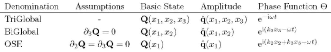
In linear stability theory, the perturbation term is usually written as the product of an amplitude function and a phase function, q = qO. Table (1) summarizes the different instability approaches arranged by increasing constrains to the basic flow. These different approaches are explained in the next subsections in more detail.

Table 1. Classification of linear stability t h e o r y concepts for analysis of a steady s t a t e Q.

Denomination Assumptions Basic State Amplitude Phase Function © TriGlobal

BiGlobal OSE

-¿>3Q=0 ¿>2Q = ¿>3Q = = 0

Q(x1,x2,x3)

Q ( x i , x2) Q(*l)

q(x1,x2,x3)

q(xi,x2) q(xi)

e-iut

ei(k3x3—ut)

eÍ(k2X2 + k3X3—Ut)

Using that approach, what is finally obtained is an eigenvalue problem for ui as eigenvalues and q as eigenvectors. The eigenvalues will have a real part, that will be the growth rate and a imaginary part that will be the frequency of the oscillations. In the notation used, u> is multiplied by —i, that means that the real part of ui will actually be the frequency changed of sign, and the growth rate will be the imaginary part. This option here, is called temporal amplification theory, and it is the only one applicable to TriGlobal. For the other two approaches, however, there are also wavenumbers (fe¿) that have to be taken into account. For temporal theory, they have to be all given and real, in order to have sinusoidal movement in the homogeneous directions. This method gives the growth or decay in time of the perturbations.

On the other hand, it exists the spatial theory. It consist of analyzing the problem using one of the wavenumbers as complex eigenvalues and leaving the frequency real. When spatial theory is selected, growing or decay may be found in the direction of the wavenumber that is calculated, given a frequency of oscillation. It cannot be used in TriGlobal, because it does not have any homogeneous direction. If the OSE approach is taken, it needs to be given a real wavenumber for one of the homogeneous directions. Fürthermore, it should be taken into account that directional derivatives are second order, and then, the eigenvalue problem to solve will have eigenvalues to the power of two, with the consequent difficulties of solution. This complication, however, does not add significant aspects to the matter and will not be discussed any further in this work. For an interesting review of temporal and spatial theory, applied to local stability, see Mack.17

II.B.l. Two Dimensions, BiGlobal

If the dependence in the third direction is neglected, the two-dimensional parallel flow is assumed and the corresponding stability analysis is called BiGlobal instability (see Theofilis ' for a review). Assuming that the basic flow is now dependent on two out of the three spatial coordinates (see table 1):

Q=[U,V,W,Pf(x,y), (17)

the coeflicients of the LNSE. (Eq. (15)) are z-independent, and modal perturbations now get the form

q ( x , y , z , t ) = q ( x , y ) ei^ - "í) (18)

and now there are derivatives in two dimensions.

-Í0JÚ + UÜX + VÚy + ifíWÚ + ÜUX + íjUy = ~px + —(ÚXX + Úyy

ríe

-iujv + Uvx + Vvy + \(3Wv + üVx + vVy = -py + -f—(vxx +

tie

>w + Uwx + Vwy + iftWw + üWx + vWy = -i/3p + —- (wxx + Jvv

fie uvv •/32ú)

p2v)

-/32w)

(19)

ux+vy + i/3w = 0

This can be w r i t t e n as an eigenvalue problem with [ü, v, w,p]T as eigenvectors a n d u> as eigenvalues.

T h e disturbances are three-dimensional, b u t a sinusoidal dependence is assumed only in t h e homogeneous z-direction, with t h e periodicity length Lz = 2TT//3. E q s . (19) can be again w r i t t e n in m a t r i x form.

/ ¿2D + Ux

v

x

w

x

u„

c

ID

Wy V„

v

x

\

Vy

i/3

i/3 0 )

C

0

0

ID

í

ü\

/ iw 0 0 0 \

\PJ V w 0 0 iw 0 0 \U1 0 0 V w / ú \

\ 0 0 0 0 /

(20)

\PJ

where LID = UVX + VVy + Wifí — -^(Vxx + Vyy — /32). Here /3 is a wavenumber parameter, related with t h e periodicity length along t h e homogeneous spatial direction, z.

III. Results

T h e results are collected in this section for t h e two vortex wake. First a simple 2D point vortex analysis is done, later a 3D filament vortex analysis is carried out, which is t h e same as Crow, a n d later t h e same problem is studied by means of s t a n d a r d linear modal stability (BiGlobal).

I I I . A . 2 D P o i n t V o r t e x A n a l y s i s o f T w o C o u n t e r R o t a t i v e V ó r t i c e s

If t h e eigenvalues of t h e problem shown in Eq. (6) are calculated analytically, it is obtained t h a t there is only

one quadruple eigenvalue — \UJ = 0. Note t h a t a numerical algorithm m a y fail here due t o t h e singularity of t h e m a t r i x . These four nuil eigenvalues means t h a t if any p e r t u r b a t i o n is introduced, it will b e maintained, neither amplified or d a m p e d , and, for any p e r t u r b a t i o n of t h e initial configuration t h e distance p e r t u r b e d will remain constant. Due t o t h e simplicity of t h e problem, this conclusión could have been obtained by simple deduction, without any m a t h e m a t i c a l analysis, b u t it is always i m p o r t a n t t o find t h e m a t h e m a t i c a l proof of t h e results.

I I I . B . 3 D P o i n t V o r t e x A n a l y s i s o f T w o C o u n t e r R o t a t i v e V ó r t i c e s

In this case, t h e eigenvalue problem t h a t defines t h e problem t o analyze, is given by Eq. (11). However, this equation depends of two p a r a m e t e r s , k a n d d, so t h e y have been defined before. Once valúes are given t o t h e two of them, t h e solution is straightforward. However, t h e physic of t h e problem has t o b e in m i n d for t h e selection of t h e p a r a m e t e r s , as any r a n d o m selection m a y not b e physical. This section solves, basically, t h e same problem as Crow, b u t more details of t h e solution are obtained, which will be of great use t o compare with other m e t h o d s .

í/k > d, which means that for a given d, k should be approximately smaller than the inverse of it. For

example, for a valué of the cutoff of 0.1, the wavenumber should be less than 10 and for a cutoff of 0.5, the wavenumber should be less than 2.

Note that the limits obtained above are approximated valúes and they could be exceeded, but they should be always keep in mind.

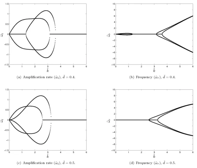
The eigenvalue problem is now solved for k from 0 to 6 and five selections of d: 0.1, 0.2, 0.3, 0.4 and 0.5. Note that d = 0.2 is in the limit of validity of the parameter and the higher valúes will be outside this limit. However, the results of these parameters are obtained to see how the problem changes when the cutoff does, but it should not be forgotten that the validity of the results in that range is at least doubtful. The resulting valúes of the amplification rate (w¿) and frequency (¿>r) have been collected in figures 1 and 2, where the upper half of figures l(c), l(e) and 2(a) coincide with figure 9 of Crow.1

The four eigenvalues are always in pairs and either they are real or imaginary, but they have never the two components. The couples have the same valué with positive and negative sign. That is, when there is a growing mode, there exist a decaying mode, and the neutral eigenvalues appear as a complex plus a complex conjúgate.

Lets introduce now the shape of the modes with the help of figures 3, 4 and 5. The first mode that grows for small k is always a symmetric mode, shown in figures 4(a) and 5(a). For small d it appears far from the asymmetric growing mode, but as d mercases, this mode, represented in figure 5(c), moves closer to small wavenumbers, appearing from any positive k for a cutoff equal to 0.5 as figure 2(c) shows. Also for small cutoff parameters, a second región of symmetric instability appears near to the región of asymmetric instability, but this región approaches faster to the first región of instability as the cutoff increases becoming a single symmetric instability región for a valué in between 0.2 and 0.3 of the cutoff distance. In the regions that either the symmetric or asymmetric mode are neutrally stable, two modes with frequency appear, that neither grow or decay, but move at a definite frequency in time both upstream and downstream.

To conclude this section of results, it could be said that the results as the wavenumber tends to zero are also zero, as was proved in the 2D analysis carried out previously.

III.C. BiGlobal Analysis of Two Counter Rotative Vórtices

The BiGlobal analysis consists basically of solving the eigenvalue problem defined in Eq. (20). However, this solution is not straightforward and some considerations have to be done before. The way to discretize the derivatives is important and various approaches are possible. Chebyshev-Gauss-Lobatto discretization is very common, but has some drawbacks as the matrices that uses are full and then is less suitable for sparse algebra. On the contrary, high order finite differences can be used with high accuracy (see Paredes et al. ) and they can take all the advantage of sparse solvers. This discretization method is an essential tool to be able to obtain quality results in standard computers. The way to calcúlate the two dimensional operators is done by the Kronecker product, but that and other considerations related to the high order finite differences and its discretization are general of the method and can be seen in more detail in the mentioned paper by Paredes et al. In addition, some boundary conditions have to be imposed to the problem, which is a delicate aspect that will be analyzed in depth. In addition, a basic flow and a wavenumber ¡3 have to be selected, aspect, the first of them, that will be commented later. It is also important to mention that an Arnoldi algorithm is used to obtain only a few eigenvalues in much shorter time, decreasing also the problem size.

III. C. 1. Baste Flow

The basic flow is a field for U, V, W and its derivatives, which must be a stationary solution of the Navier-Stokes equations. Sometimes it could be given analytically, and it could also be obtained as a solution of a 2D DNS code when the final result do not vary in time.

¡ 3

(a) Amplification rate (w¿), d = 0.1. (b) Frequency (uir), d = 0.1.

¡ 3

A

\J

(c) Amplification rate (w¿), d = 0.2. (d) Frequency (uir), d = 0.2.

'3 '3

0 1 2 3 4 5 6

k

(e) Amplification rate (£>¿), d = 0.3. (f) Frequency (¿)r), d = 0.3.

¡ 3

(a) Amplification rate (w¿), d = 0.4. (b) Frequency (uir), d = 0.4.

¡ 3

(c) Amplification rate (w¿), d = 0.5. (d) Frequency (uir), d = 0.5.

Figure 2. Amplification rate (úí) and frequency (ujr as a function of the wavenumber k for d: 0.4 and 0.5.

(a) Symmetric, positive (b) Symmetric, negative (c) Asymmetric, positive (d) Asymmetric, negative

(a) Symmetric, growing (b) Symmetric, decaying (c) Asymmetric, positive (d) Asymmetric, negative

Figure 4. The four modes for k = 1.5 and d = 0.3. Two neutral eigenvalues, one growing and one decaying.

(a) Symmetric, growing (b) Symmetric, decaying (c) Asymmetric, growing (d) Asymmetric, decaying

Figure 5. The four modes for k = 3 and d = 0.4. Two growing eigenvalues and two decaying.

parameter q = ra/(27rWo) that is what gives them the ñame.

/ ( * - ^ ) W \ yTa (

U{x,y) 1 - e

V(x,y) = I 1 — e

W(x,y) = 0

(o,-Xa)¿+y¿

J 2Tv((x-Xay+yi)

(x - Xa)Ta _

2 ^ ( ( x - X0)2+ y2)

(ic + Xa)¿+y¿

1 - e

(oi + Xa)¿+y¿

1 - e

V^a

) 2^((x + X0)2+ y2)

(x + Xa)Ya

2^((x + X0)2 + y2)

(21)

( x - Xa) ^ + ¡,^ U{x,y) = - | 1 - e

V(x,y) = í 1 — e

W(x,y) = ^ 0 ( 0 + 6

V^a (ic + Xa)¿+y¿

(o,-Xa)¿+y¿

J 2^((x-X

0

)

2

+y

2

)

(X - Xg)Ya

2 ^ ( ( x - X0)2+ y2)

1 - e y^a

(oi + Xa)¿+y¿

1 - e

J 2^((x + X

0

)

2

+y

2

)

(x + x

a

)r

a

2^((x + X0)2 + y2)

( x - Xa) ^ + ¡ , ^

+ W0 U + e

(x + Xa) ^ + ¡,^

(22)

III. C. 2. Boundary Conditions

The boundary conditions for the variables ü, v and w are very easy to impose in the case that the two vórtices are taken inside the domain and the boundaries are kept far away enough. In that case, Dirichlet conditions are imposed on all the boundaries. However, the symmetry of the problem allows to calcúlate the solution as the sum of symmetric and antisymmetric solutions of only one half. In that case, two different sets of conditions have to be imposed. Symmetry conditions mean Neumann boundary conditions, while antisymmetry mean Dirichlet boundary conditions.

Symmetric case: v and w are symmetric, while u is antisymmetric:

u{x,y) = -ü{-x,y)

ij{x,y)=v{-x,y) (23) w(x,y) = w(-x,y)

Antisymmetric case: u is symmetric, while v and w are antisymmetric:

ü(x,y) = ü(-x,y)

v{x,y) = -v(-x,y) (24) w(x,y) = -w(-x,y)

III. G. 3. Comparison Full boundary and Half Boundary

First of all, a validation case for the boundary conditions is selected. It will be a case for low Re and q of order unity, which lead some instabilities. The exact valúes of the problem are the following:

fie = 1 0 0 , q = 0.475, a = 0.0, Xa = 2.0, a0 = 1.0, ¡3 = 0.418

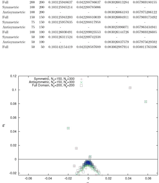
Convergence of the solution is shown in table 2 for the first two unstable eigenvalues. Good convergence is seen for both eigenvalues, but the symmetric boundary seems to have better behavior. Figure 6 highlights that the unión of the symmetric and antisymmetric modes is the same result as the full solution. Similarities can be found with figure 4b of Hein and Theofilis. These spectra have been calculated with high order finite differences of order 8. The Krilov space was only of 100 points, and that is the reason because the number of eigenvalues is not very big and the continuous part of it is not very well converged, although it is not needed either.

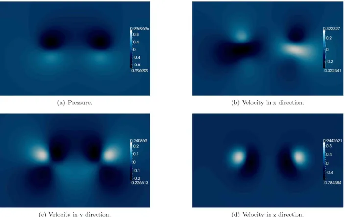
The modes are complex and therefore, as the grid is not the same for the case of full domain and the case of half domain, the eigenvectors are moved one phase and then they do not look the same for half and full domain. However, the reconstruction in space and time will give the same Figures 7 and 8 represent the valué of the imaginary part of the modes, only for the full domain simulations. There, the kind of boundary condition in the center is appreciated, where it can be seen that all the variables, but u follow the symmetry or antisymmetry of the mode, while u does the opposite.

III. C.4- Effsct of adding the descent speed

The results presented before are calculated without adding the descent speed of the vórtices to the basic flow and for an analytic and imposed base flow. In this paragraph it is shown how the descent speed,

Vd = q/2Xa = 0.119, even if small, displaces the spectrum. For that purpose, figure 9 is shown, where

convergence have been analyzed again, as well as the symmetric and antisymmetric meshes are used to show whether the eigenvalues are symmetric or antisymmetric. The shape of the first two modes (not shown here) is very similar to those without descent speed added (again symmetric and antisymmetric respectively), and therefore these two modes correspond to the ones with descent speed equal zero.

IV. Conclusión

Table 2. Table of convergence for t h e two more u n s t a b l e modes, Mesh Symmetric Antisymmetric Full Symmetric Antisymmetric Full Symmetric Antisymmetric Full Symmetric Antisymmetric Full Nx 150 150 200 100 100 150 75 75 100 50 50 50 Ny 300 300 200 200 200 150 150 150 100 100 100 50

Mode 1 LUÍ

0.103125944794 -0.103125948637 0.103125945214 -0.103125943203 0.103125957635 -0.103126030491 0.103126311524 -0.103142154419

Mode 1 tür

0.042288780713 -0.042288786637 0.042288785006 -0.042288810039 0.042288817958 -0.042289023553 0.042289742338 -0.042328587689

Mode 2 UJÍ

-0.083025955469 0.083026013284 -0.083026064183 0.083026004911 -0.083025996071 0.083026144726 -0.083026837579 0.083062987914

Mode 2 ujr

-0.057975378840 0.057969180155 -0.057975206122 0.057969173492 -0.057963434941 0.057969326685 -0.057975629592 0.058011763106 0.12 0.08 0.06 0.04 0.02 -0.02

(a) Pressure. (b) Velocity in x direction.

(c) Velocity in y direction. (d) Velocity in z direction.

Figure 7. Imaginary part of the four components of the first symmetric mode for the valúes specified above.

(a) Pressure. (b) Velocity in x direction.

(c) Velocity in y direction. (d) Velocity in z direction.

Symmetric, Vd, Nx=150, Ny=300 +

Antisymmetric, Vd, Nx=150, Ny=300

Full Domain, Vd, Nx=200, N =200 •

0.14

0.12

0.1

0.08 0.06 0.04 0.02

Full Domain, Nx=200, Ny=200

-i • -

A

-0.06 -0.04 -0.02 0

(Or

0.02 0.04 0.06

Figure 9. Spectrum to show the effect of the descent speed, in this case, V¿ = 0.11875.

methodology, which, also in this case, have demonstrated that the use of this new upgrade can reproduce or even improve previous results with very little computational resources.

The advantages of the point vortex stability methods are the simplicity, which means easy to compute, and the small number of parameters. By contrast, due to that facts, the real problems cannot be modeled accurately.

The BiGlobal method, on the other hand, offers a wide range of parameters to analyze, and different options when modeling the equations. These are both its advantages and disadvantages, because the number of parameters, among them the viscosity, allows the possibility to model the problem with more accuracy, but if not done properly, might not lead to interesting conclusions. In that line, this work has analyzed the effect of some of the parameters, but much more can be done in that área.

Acknowledgments

Support of the Secretaría de Estado de Investigación, Desarrollo e Innovación of the Spanish Ministry of Economy and Competitiveness through Grant MICINN-TRA2009-13648: "Metodologias computacionales

para la predicción de inestabilidades globales hidrodinámicas y aeroacusticas de flujos complejo" is gratefully

acknowledged.

References

1Crow, S. C , "Stability Theory for a Pair of Trailing Vórtices," AIAA J., Vol. 8, 1970, pp. 2172-2179.

2Crouch, J. D., "Instability and Transient Growth for Two Trailing-Vortex Pairs," J. Fluid Mech., Vol. 350, 1997, pp. 311—

330.

3Kármán, T. V., "Uber den mechanismus des widerstandes, den ein bewegter kórper in einer flüssigkeit erfahrt," Nachr.

Ges. Wissenschaft. Gottingen, 1911, pp. 509—517.

4K á r m á n , T. V., "Uber den mechanismus des widerstandes, den ein bewegter kórper in einer flüssigkeit erfahrt," Nachr.

Ges. Wissenschaft. Gottingen, 1912, pp. 547—556.

5 Jiménez, J., "Stability of a pair of co-rotating vórtices," Phys. Fluids, Vol. 18 (11), 1970, pp. 1580—1581.

6Fabre, D., Cossu, C , and Jacquin, L., "Spatio-temporal development of the long and short-wave vortex-pair instabilities,"

Phys. Fluids, Vol. 12, No. 5, MAY 2000, pp. 1247-1250.

7Hein, S. and Theofllis, V., "On instability characteristics of isolated vórtices and models of trailing-vortex systems,"

Comp. & Fluids, Vol. 33, No. 5-6, JUN-JUL 2004, pp. 741-753, Conference on Applied Mathematics for Industrial Flow Problems, LISBON, PORTUGAL, A P R 17-JUL 20, 2002.

8Rodríguez, D. and Theofllis, V., "Massively Parallel Solution of the BiGlobal Eigenvalue Problem Using Dense Linear

Algebra," AIAA J., Vol. 47, No. 10, O C T 2009, pp. 2449-2459, AIAA 46th Aerospace Sciences Meeting and Exhibit, Reno, NV, JAN 07-10, 2008.

9Broadhurst, M., Theofllis, V., and Sherwin, S., "Spectral element stability analysis of vortical flows," Sixth IUTAM

Symposium on Laminar-Turbulent Transition, edited by Govindarajan, R, Vol. 78 oí Fluid Mechanics and its Applications, Int Union Theoret & Appl Mech, SPRINGER, PO BOX 17, 3300 AA D O R D R E C H T , NETHERLANDS, 2006, pp. 153-158, 6th IUTAM Symposium on Laminar-Turbulent Transition, Bangalore, INDIA, DEC 13-17, 2004.

1 0Gonzalez, L. M., Gómez-Blanco, R., and Theofllis, V., "Eigenmodes of a Counter-Rotating Vortex Dipole," AIAA J.,

Vol. 46, No. 11, NOV 2008, pp. 2796-2805, AIAA 37th Fluid Dynamics Conference, Miami, FL, JUN 25-28, 2007.

^ P a r e d e s , P., Hermanns, M., Clainche, S. L., and Theofllis, V., "Order 104 speedup in global linear instability analysis

using matrix formation," Comput. Methods Appl. Mech. Engrg., Vol. 253, 2013, pp. 287—304.

1 2Rennich, S. C. and Lele, S. K., "Method for Accelerating t h e Destruction of Aircraft Wake Vórtices," Journal of Aircraft,

Vol. 36, No. 2, 1999, pp. 398-404.

1 3Widnall, S. E., Bliss, D. B., and Zalay, A., Aircraft Wake Turbulence and its Detection, Plenum, New York, 1971, p. 305.

14Theofllis, V., "Advances in Global Linear Instability Analysis of Nonparallel and Three-Dimensional Flows," Prog. in

Aero. Sciences, Vol. 39 (4), 2003, pp. 249-315.

1BTheofllis, V., "Global linear instability," Annu. Rev. Fluid Mech., Vol. 43, 2011, pp. 319-352.

1 6Butler, K. and Farrell, B. F., "Three-Dimensional Optimal Perturbations in Viscous Shear Flow," Physics of Fluids,

Vol. 4 (8), 1992.

1 7Mack, L. M., "Boundary-Layer Stability Theory," AGARD Report No. 709. Special Course on Stability and Transition

of Laminar Flow, 1984, pp. 3 - 1 - 3 - 8 1 .