Article
Managing Traffic Flows for Cleaner Cities:
The Role of Green Navigation Systems
Fiamma Perez-Prada1,*, Andres Monzon2and Cristina Valdes3
1 Transport Research Centre (TRANSyT), Escuela de Ingenieros de Caminos, Canales y Puertos, Universidad Politécnica de Madrid, Ciudad Universitaria, 28040 Madrid, Spain
2 Transport-Civil Eng. Department, Escuela de Ingenieros de Caminos, Canales y Puertos, Universidad Politecnica de Madrid, 28040 Madrid, Spain; [email protected]
3 Empresa Municipal de Transportes de Madrid, 28007 Madrid, Spain; [email protected] * Correspondence: [email protected]; Tel.: +34-91-336-6708
Academic Editor: K.T. Chau
Received: 24 February 2017; Accepted: 7 June 2017; Published: 9 June 2017
Abstract: Cities worldwide suffer from serious air pollution problems and are main contributors to climate change. Green Navigation systems have a great potential to reduce fuel consumption and exhaust emissions from traffic. This research evaluates the impacts of different percentages of green drivers on traffic, CO2, and NOxover the entire Madrid Region. A macroscopic traffic model
was combined with an enhanced macroscopic emissions model and a GIS (Geographic Information Systems) to simulate emissions on the basis of average vehicle speeds and traffic intensity at the link level. NOxemissions are evaluated, taking into account not only the exhaust emissions produced by
transport activity, but also the amount of the population exposed to these air pollutants. Results show up to 10.4% CO2and 13.8% NOxreductions in congested traffic conditions for a 90% penetration of
green drivers; however, the population’s exposure to NOxincreases up to 20.2%. Moreover, while
traffic volumes decrease by 13.5% for the entire region, they increase by up to 16.4% downtown. Travel times also increase by 28.7%. Since green drivers tend to choose shorter routes through downtown areas, eco-routing systems are an effective tool for fighting climate change, but are ineffective to reduce air pollution in dense urban areas.
Keywords:eco-routing; green navigation; traffic emissions; climate change; air pollution; co-benefits; trade-offs; ICT; CO2; NOx
1. Introduction
ICT (Information Communication Technology)-based strategies applied to traffic have brought about new possibilities to improve traffic performance in urban environments, all while reducing their externalities. The emissions reduction potential of ICT-based solutions has traditionally been viewed as secondary to impacts on traffic safety and congestion. Nevertheless, recently, different researchers have been studying the effects of these new technologies on fuel consumption and CO2 emissions [1–4].
Out of the different ICT-based strategies, Green Navigation (GN) systems have shown important fuel consumption and CO2 reductions when compared to typical travel-time and monetary-cost minimization routing strategies [5–7]. These reported reductions were largely attributed to vehicle travel distance reductions, which, when eco-routing is applied to an entire metropolitan area, lead to an increase in emissions on urban streets, due to transferring traffic to shorter routes [7]. GN systems produce global benefits in terms of CO2. However, the impact of GN systems applied at the city-wide level on the reallocation of emissions and its effect on air pollution is not yet well understood.
This research aims to bridge this gap and evaluate the impacts of GN systems on air pollution, taking into account the varying influence of transport emissions on the urban environment [8]. Our hypothesis is that GN systems provide clear benefits to mitigate greenhouse gases (GHG) emissions, but they could be ineffective at reducing local air pollution in urban environments. To this end, the research evaluates the environmental and traffic performance impacts of GN Systems, with a special focus on the analysis of climate change and air pollution co-benefits and conflicts. Thus, we calculate both CO2 and NOx emissions from the Madrid Metropolitan area assuming
different percentages of GN drivers in the Madrid Region. Unlike other papers, we also take into account the local impact of air pollutants; hence, we model the population exposure to NOx
emissions. This research provides local policy makers and city managers with insights to design and properly implement transport reduction strategies, maximizing climate change and air pollution reduction synergies.
2. Climate Change and Air Pollution: Co-Benefits and Conflicts of Transport Emissions Reduction Strategies in Urban Areas
Cities worldwide suffer from serious air pollution problems and are main contributors to climate change, consuming about two-thirds of the world´s overall energy and emitting an estimated 70% of the world´s anthropogenic GHG emissions [9]. Globally, transportation is responsible for 23% of anthropogenic CO2emissions and 54% of NOxemissions, of which 75% and 72%, respectively, are
attributable to road transport [10]. Road traffic is a major source of GHG emissions, and the largest contributor to air pollutant emissions in urban environments. Moreover, the predicted growth in the urban population and transport activity will further contribute to increasing transport emissions in the near future [11].
The role of sustainable urban mobility strategies in climate change mitigation has drawn increased interest in recent years: a number of authors are examining different transport strategies to reduce GHG emissions [12–16].
Traffic emissions have different spatial and duration impacts [17]: While CO2emissions are a global problem with large-scale impacts—no matter where the emissions are produced, all of them contribute to climate change—short lived GHGs such as ozone have a regional effect. On the other hand, traffic air pollution has important regional and local impacts. Pollutant concentrations decrease in concentration as they are transported by the wind and vehicle movement turbulence from the source [18]. Increased health risks for populations located near major roadways and transportation infrastructures, particularly in densely populated urban areas, have been continuously reported [19]. However, transport planning has usually tackled them in a similar way, considering that most of the strategies designed to reduce GHGs emissions also reduce air pollutants and vice-versa and do not account for the spatial variation of transport emissions,. This can be observed through the gross indicators habitually used to measure the environmental impact of different transport projects: tons of reduced CO2, kg of NOx, or kg of PM. To obtain these indicators, we only need to take traffic activity
attributes into account. However, when analyzing the impacts of the projects on air pollution, it is important to take their greater impact on highly-populated areas into account. Therefore, it is necessary to develop indicators that also take the spatial impacts of transport emissions, particularly at an urban level, into account [20].
Transport policies designed to avert climate change show co-benefits for air pollution mitigation [21–28]; however, they also present conflicts. A well-known case is the shift to diesel cars, which not only delivered less CO2reductions than expected [29,30] but also increased air pollution. For example, a study in Ireland showed how a car taxation policy promoting the purchase of lower CO2emitting cars could lead to a higher share of fuel-efficient diesel vehicles, with up to 7% in CO2reductions, but a 28% increase in NOx emissions [31]. The use of biofuels also has potential
trade-offs regarding air pollution, particularly regarding NOxemissions. The literature illustrates two
temperatures of combustion [32,33] while others reported lower emissions due to the lower amount of premixed fuel and peak burning temperature compared to diesel and gasoline fuels [34,35]. A review on the impacts of biofuel exhaust emissions can be found in [36]. Concerning electric vehicles, studies showed that they have a directly positive impact on pollution in urban environments, since exhaust emissions are not produced during the operation of the vehicle [37,38]. Studies also reported the need for further regulation to address the non-exhaust emissions [37] of electric vehicles in the future, and the importance of taking into account the electricity mix of the countries [39].
Measures directly affecting traffic performance were also analyzed, from the combined perspective of climate change and air pollution. For example, traffic-calming measures reported increases in CO2 and NOx[40,41]. Traffic calming can provide emissions reductions only if they generate a reduction
in traffic activity, or a shift toward more efficient transport modes. In a study conducted in Madrid City, Garcia-Castro et al. [42] showed that while under low and medium congested traffic conditions eco-driving leads to reductions of up to 2.3% in CO2and of up to 4.3% in NOxemissions, under
highly-congested traffic conditions, emissions increase by up to 1.3% and 0.5%, respectively. In Belgium, a study showed reductions of about 10% in NOxand CO2, thanks to implementing a green-wave signal coordination scheme along an urban arterial road [43]. Cohen et al. [44] reported global environmental benefits from a speed-reduction strategy in segments along different Lille freeways, and Perez-Prada and Monzon [8] reported a 14.4% and 16.4% reduction in CO2and NOxemissions, respectively, thanks
to implementing a reduced speed limit on an urban ring-road. Regarding road capacity increases, Monzon et al. [45] predicted a reduction in GHGs and air pollutants in Madrid after the renovation of its inner ring-road. An ex-post study [46] confirmed this trend after the renovated beltway had been operating for three years (short-term). However, other studies [47] suggested an increase in emissions in the long run after a road capacity increase.
Green Navigation (GN) systems, or eco-routing systems, provided routing recommendations based on calculation of the environmental impact and the real-time traffic situation, i.e., for a given origin and destination, they provide the route that minimizes fuel consumption. Previous research [1,7] reported up to 8.2% in CO2savings under highly congested conditions, and up to 9.5% in CO2savings in free-flow or low-congested conditions. These studies also reported increasing CO2savings as the level of “green drivers” increases, and the vehicle-km travelled decreases, due to the selection of shorter routes. In a later work, Valdes et al. [7] indicated that those benefits were mostly concentrated on freeways and highways, while urban streets and extra-urban roads experience an increase in emissions, due to the transfer of traffic to shorter routes. This research suggested that, since length has an important effect on fuel consumption, green drivers choose routes similar to the minimum length, although this may imply crossing the downtown area or selecting a road with lower speed than a highway. Those eco-routing studies show the effectiveness of that measure to reduce fuel consumption, and therefore CO2emissions.
Based on the results of previous works, the present research argues that GN systems present clear benefits for combating climate change, but that they could be ineffective for reducing air pollution in urban environments. To this end, we will analyze the impacts of GN systems on CO2and NOx
emissions in the city of Madrid, taking the different spatial impacts of GHG and air pollutant emissions into account in this research.
3. Method
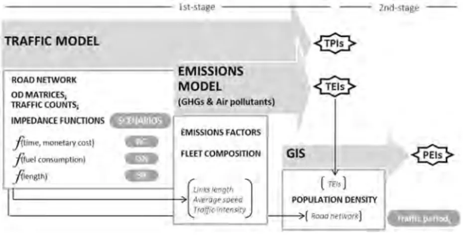
The interaction of the models takes place in two phases, summarized in Figure1. The first stage follows the ICT-Emissions project methodology [48]. It assesses CO2emissions of ICT-based strategies at the macro-scale level, linking the widespread macroscopic emissions model, COPERT, to a macroscopic traffic model. The traffic demand model fulfills three functions at this stage. First, it is used to generate the different scenarios under analysis. Base-case (BC) scenarios represent the current traffic situation for each of the traffic periods analyzed, while Green Navigation (GN) and Shortest-Route (SR) scenarios are obtained by varying the traffic model impedance function. SR scenarios will only be used to understand to what extent the GN impedance function, which is designed to minimize fuel consumption, takes changes in speed and traffic intensity into account, and not only changes in itinerary lengths. Second, it provides inputs for the emission model (links lengths, average speeds, and traffic intensity). Finally, it generates the TPIs used in the evaluation. On the other hand, the emissions model generates TEIs based on EFs, fleet composition, and the inputs of the traffic model. TEIs only take traffic activity and fleet composition into account.
Energies 2017, 10, 791 4 of 18
Shortest-Route (SR) scenarios are obtained by varying the traffic model impedance function. SR scenarios will only be used to understand to what extent the GN impedance function, which is designed to minimize fuel consumption, takes changes in speed and traffic intensity into account, and not only changes in itinerary lengths. Second, it provides inputs for the emission model (links lengths, average speeds, and traffic intensity). Finally, it generates the TPIs used in the evaluation. On the other hand, the emissions model generates TEIs based on EFs, fleet composition, and the inputs of the traffic model. TEIs only take traffic activity and fleet composition into account.
Figure 1. Methodology flow chart.
The second stage of the model evaluates traffic emissions, taking their effect on the population into account. We use a GIS to calculate PEIs, weighting TEIs by population concentrations near each roadway. The higher the PEI values, the worse the impact of the air pollutant emissions. The GIS needs inputs from the traffic model (road network) and the emissions model (TEIs), and information regarding population densities.
3.1. Traffic Scenarios
For the assessment, three different scenarios have been considered, varying the traffic model impedance function. The model impedance function, also known as the model objective function, is the key factor in driver´s route choices. It assigns the effort connected to each route or path. Usually, this effort is measured in terms of travel time. Additional properties, such as travel expenses, can be converted into travel time units, and considered within the travel impedance function [49]. The traffic assignment selects the routes that minimize the impedance function.
The scenarios considered are:
The BC represented the existing traffic situation. It will assign the typical impedance function for conventional drivers, which is based on time and cost.
The GN scenario assigned an impedance function defined in terms of fuel consumption, which is directly related to CO2 emissions, i.e., the assignment will seek results that minimize fuel consumption, and therefore CO2 emissions, as well. The ICT-Emissions project tested five different fuel consumption functions from different studies, and the one that best performed under congested traffic conditions was selected, i.e., the default fuel consumption function of COPERT (g/km), expressed as a function of time (g/s) [1,7]:
= ( ) (1)
where: IGN is the GN impedance function expressed in seconds, FC is the COPERT default fuel consumption function expressed in g/s as:
Figure 1.Methodology flow chart.
The second stage of the model evaluates traffic emissions, taking their effect on the population into account. We use a GIS to calculate PEIs, weighting TEIs by population concentrations near each roadway. The higher the PEI values, the worse the impact of the air pollutant emissions. The GIS needs inputs from the traffic model (road network) and the emissions model (TEIs), and information regarding population densities.
3.1. Traffic Scenarios
For the assessment, three different scenarios have been considered, varying the traffic model impedance function. The model impedance function, also known as the model objective function, is the key factor in driver´s route choices. It assigns the effort connected to each route or path. Usually, this effort is measured in terms of travel time. Additional properties, such as travel expenses, can be converted into travel time units, and considered within the travel impedance function [49]. The traffic assignment selects the routes that minimize the impedance function.
The scenarios considered are:
• The BC represented the existing traffic situation. It will assign the typical impedance function for conventional drivers, which is based on time and cost.
IGN =FC(vCur)x tCur (1)
where:IGNis the GN impedance function expressed in seconds,FCis the COPERT default fuel consumption function expressed in g/s as:
FC=av5Cur+bv4Cur+cv3Cur+dv2Cur+evCur+f (2)
a=−3.29612×10⁻¹,b= 1.097×10⁻⁷,c=−1.1893×10⁻⁵,d= 5.30345×10⁻⁴,e=−1.56253×10⁻³,
f = 0.256344,vCuris the link average speed calculated in the traffic model in km/h, andtCuris the link travel time calculated by the traffic model in seconds.
• A SR scenario has also been considered. This last scenario assigned an impedance function defined exclusively in terms of trip length.
It is not realistic to assume that all the vehicles in the network would be equipped with eco-routing navigation systems; therefore, different levels of penetration will be considered in this research. Five GN scenarios representing different percentages of eco-routing drivers will be compared to the BC. The penetration rates selected for study are 10% (GN10 scenario), 25% (GN25), 50% (GN50), 75% (GN75), and 90% (GN90). GN scenarios will consist of a combination of GN drivers and conventional drivers; the origin-destination (OD) matrix has been divided into two, one for GN drivers and the second for conventional drivers. For example, in the GN25 scenario, 75% of the OD matrix is assigned to conventional drivers, and the other 25% to green drivers according to Equation (1). The same reasoning applied to the SR scenarios (five penetration rates and assignment of OD matrices between the shortest route drivers and the conventional ones).
Navigation systems provide eco-routing recommendations based on a calculation of the environmental impact and the real-time traffic situation. The GN-scenario assignment process was designed to continuously collect new traffic conditions and then, to allow for different route alternatives, taking this new traffic situation into account. First, heavy vehicles and conventional car drivers were assigned to the network, and subsequently, the impedance function of green drivers is calculated for the new traffic levels and average speeds. Next, green drivers were assigned to the network in 10 steps, and after each of the stages, the impedance function was calculated again to show the new traffic conditions. This implies that, in every step of the GN demand segment assignment, the impedance function is updated with the new traffic situation, and henceforth, routing recommendations will be modified consequently. In each stage, 10% of the OD matrix corresponding to green drivers is assigned.
3.2. Assessment Indicators
The model outputs are three different types of indicators designed to understand the impact of eco-routing systems on traffic, climate change, and air pollution: traffic performance indicators (TPIs), traffic emissions indicators (TEIs), and population exposure indicators (PEIs).
Traffic performance was evaluated in terms of volume (VKM) and travel times (VEH). In view of the fact that GN systems do not affect the geometry of the network (link length and capacity), changes in traffic volume also represent changes in saturation rates (traffic intensity divided by section capacity). The TPIs used for the assessment are:
(traffic intensity divided by section capacity) and traffic volume will be used as synonyms for traffic intensity when used in relative terms, since the measurement under study does not modify the length nor the capacity of the links.
VKMi,p= N
∑
i
Ii,pli (3)
• VEH (VEhicles per Hour) represents the total travel time of all vehicles on a link or segment of the road for an average hour of the three defined periods. It is calculated as a product of the traffic intensity and travel time. See Equation (2), wheretis the travel time in hours on a specific link of the network for an average hour in the time period considered, and the rest of the terms are the same as those used in VKM.
VEHi,p= N
∑
i
Ii,pti,p (4)
Traffic emissions were evaluated in terms of CO2and NOx. CO2is the largest GHG anthropogenic emission, and NOxhas commonly been used as a proxy for traffic-related air pollution [45,46].
TEIs were calculated by the link as a product of traffic volume and theEFcorresponding to the average speed of the link for the Madrid fleet composition. See Equation (3), wheremrepresents vehicle classes (fleet composition), depending on vehicle fuel technology, engine type and technology, andkis the type of emission considered (CO2or NOx). The rest of the terms are the same as those
used before.
TEIi,p,k= N
∑
i
EF(v)k,m,i,pIi,pli,p (5)
In order to show the population exposure to air pollution, we calculated PEIs, weighting transport exhaust emissions with population density, following an approach similar to the one used by Perez-Prada and Monzon [20]. See Equation (4), whereDis the population density of the area that the link crosses over. The rest of the terms are the same as those used before.
PEIi,p,k =
∑
TEIi,p,kDi,p (6)Very complex dispersion models and detailed chemistry models are needed to develop accurate population exposure indicators that take all the variables affecting concentration levels into account, e.g., precipitation, wind speed and direction, atmospheric pressure, temperature, topography, and urban street disposition, as well as the type and height of buildings [50–53].
As explained by [20], the use of population density as a proxy for exposure levels is motivated by the fact that (i) exposure to local emissions from transport is largely a function of both the amount of traffic activity, and the number of people who regularly live or work along roadsides [50,53]; that (ii) numerous studies analyze air pollutant exposure levels at a certain distance from a high-traffic road [54,55]; and that (iii) health effects and residential proximity to high traffic roads show a correlation [51].
3.3. Attributes of Model Components in the Madrid Case Study
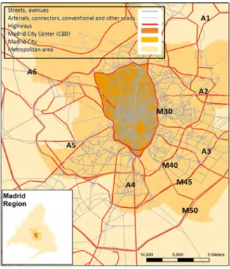
The Madrid Region is the capital of Spain and the country’s most populated region. The population of the Madrid Region amounts to about 6.5 million inhabitants, half of which live in the main city. The region is spread over an 8030 km2surface, and the population density is high in the central city, 5232 inhab./km2, and rather low in the whole region, 605 hab./km2) [56]. Figure2shows the distribution of the population within the Madrid Region.
them unfinished) encircling it: the first one is the M-30, which divides the city into two parts, the inner part—Central Area—and the peripheral districts, and it acts as a local distributor road; the second one is the M-40, which encompasses most of the city of Madrid, and is the most congested road in the Madrid metropolitan area; and the M-45 and M-50, both yet incomplete rings. Four tollways run in parallel to four of the main highways.Energies 2017, 10, 791 7 of 18
Figure 2. Population density by municipality in the Madrid Region.
3.3.1. Traffic Model Attributes
The traffic model was based on the one developed by Valdes [57] and enhanced for the ICT-Emissions project. Information regarding the model characterization and calibration can be found in [58]. The regional network consists of 15,712 road links, with a higher level of detail in Madrid City, and in particular, for the city center, i.e., inside the M30.
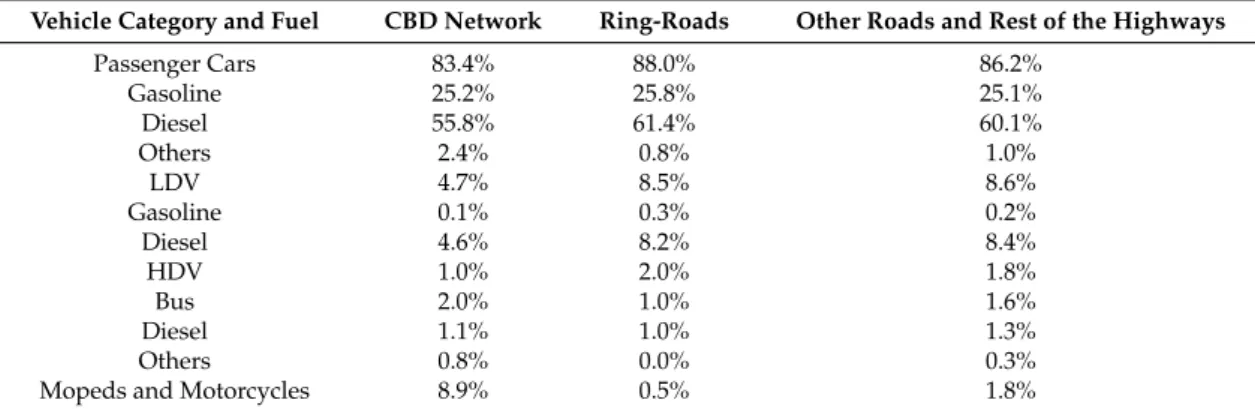
The road network was classified into three types (see Figure 3), depending on the type of road they represent.
Figure 3. Madrid road network.
Figure 2.Population density by municipality in the Madrid Region.
3.3.1. Traffic Model Attributes
The traffic model was based on the one developed by Valdes [57] and enhanced for the ICT-Emissions project. Information regarding the model characterization and calibration can be found in [58]. The regional network consists of 15,712 road links, with a higher level of detail in Madrid City, and in particular, for the city center, i.e., inside the M30.
The road network was classified into three types (see Figure3), depending on the type of road they represent.
Energies 2017, 10, 791 7 of 18
Figure 2. Population density by municipality in the Madrid Region.
3.3.1. Traffic Model Attributes
The traffic model was based on the one developed by Valdes [57] and enhanced for the ICT-Emissions project. Information regarding the model characterization and calibration can be found in [58]. The regional network consists of 15,712 road links, with a higher level of detail in Madrid City, and in particular, for the city center, i.e., inside the M30.
The road network was classified into three types (see Figure 3), depending on the type of road they represent.
Figure 3. Madrid road network.
• CBD NETWORK represents 1670 km of streets and avenues inside the M30 and accounts for 28% of the whole network.
• HIGHWAYS represent 1647 km of urban ring-roads, highways, and motorways and also account for 28% of the whole road network.
• OTHER ROADS aggregate 2560 km of conventional roads, junctions, and service lanes belonging to the peripheral, metropolitan, and regional areas, and account for 44% of the entire network.
3.3.2. Emissions Model Attributes
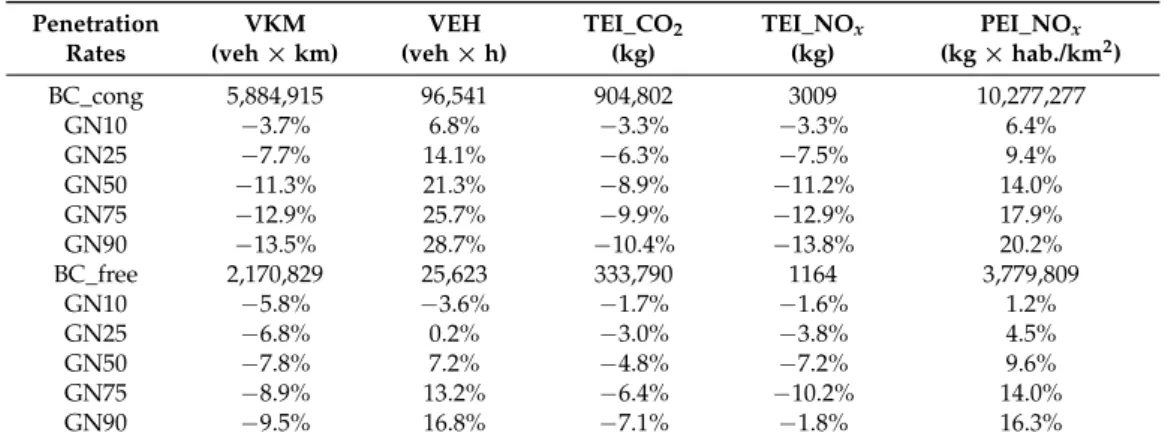
COPERT provides a straightforward expression for hot EF, based on two or three speed ranges by vehicle category. Each vehicle category is also classified according to the fuel (gasoline, diesel) and engine type, and the associated emissions reduction technology (from Conventional to Euro IV) [58]. As an innovative approach to customized urban emission assessment, the emissions model used the circulating fleet, instead of the existing fleet, to estimate emissions more accurately. The circulating fleet considers a different fleet composition by the three road-types, providing more accurate results, while the existing fleet considers that all the vehicles are equally distributed through all type of roads. However there is no data on the fleet used at different traffic periods: peak vs. off-peak. Table1shows the final distribution of the fleet throughout the network, adapted from [59].
Table 1.Madrid’s circulating fleet by category and fuel and zone distribution.
Vehicle Category and Fuel CBD Network Ring-Roads Other Roads and Rest of the Highways
Passenger Cars 83.4% 88.0% 86.2%
Gasoline 25.2% 25.8% 25.1%
Diesel 55.8% 61.4% 60.1%
Others 2.4% 0.8% 1.0%
LDV 4.7% 8.5% 8.6%
Gasoline 0.1% 0.3% 0.2%
Diesel 4.6% 8.2% 8.4%
HDV 1.0% 2.0% 1.8%
Bus 2.0% 1.0% 1.6%
Diesel 1.1% 1.0% 1.3%
Others 0.8% 0.0% 0.3%
Mopeds and Motorcycles 8.9% 0.5% 1.8%
Notes: LDV stands for Light Duty Vehicles, HDV stands for Heavy Duty Vehicles, CBD stands for Central Business District.
Passenger cars represented more than the 80% of all the vehicles in the considered zones. The share of light-duty vehicles (LDV) on urban roads was almost half that on highways and other roads. Other roads included the extra-urban network of the model, and all the highways except ring-roads. The share of two-wheel vehicles was only relevant at an urban level, where it represented almost 9%, while on ring-roads its share is almost negligible (0.5%). Finally, heavy-duty vehicles (HDV) in urban areas only accounted for 1%, while this figure was double on ring-roads (2.0%) and almost double on other roads (1.8%). The share of buses at an urban level (2.0%) doubled the bus portion on ring-roads (1.0%), and was also higher than the bus segment on other roads (1.6%).
Regarding fuel types, the highest share of gasoline cars appeared at the urban level (34.2%), which was more than 25% higher than the gasoline vehicle share on orbital highways (26.6%) and extra-urban roads (27.1%). Therefore, the share of diesel vehicles was higher on orbital motorways and other roads. It accounted for 72.5% and 71.5%, versus a 62.4% share in urban areas. The share of other types of fuels was trivial for other roads and highways, and very small for the urban network (3.3%).
3.3.3. GIS Attributes
Finally, using a GIS tool, population maps provided by the National Statistical Institute (http://www.ine.es/) were combined with the model network to assign a new link characteristic: population density. We have used information from 4341 census sections in the Madrid Region.
These sections are an official geographical reference of statistical character. Since they have basically an operational character and therefore always have to be defined by more or less fixed sizes: to be accessible to an interviewing agent for the purpose of population counts or statistical surveys, it is recommended that the size of a section does not exceed 2500 legal residents [60].
For links crossing more than one census section, the density was calculated as follows:
Link Density= ∑ N i Ai Pi
∑Ai
(7)
whereAis the area of the census section,Pis the population in the census section, andNis the total number of census sections crossed by the link.
3.4. Model Assumptions and Limitations
Some authors questioned the appropriateness of average speed models to assess emissions at a city level [61,62] since similar average speeds can be reached with different speed patterns in each link. Notwithstanding, this model was further developed for calculating emissions at a link level in urban environments [63], including (i) algorithms suitable for working with hourly time periods and for links that are hundreds of meters long; (ii) a subroutine to distribute the data among the hundreds of types of vehicles, subdivided by fuel type, age, etc. Limitations may appear for high saturation levels (e.g., >80%) and/or for very short road segments (e.g., <400 m). Moreover, as is customary, start emissions and evaporation emissions are not considered.
Due to the use of population density, PEIs are mainly residentially focused and only partially reflect exposure to air pollution, as they exclude the effects on working areas and on tourist and commercial areas that frequently exhibit higher numbers of pedestrians. Besides, PEIs do not completely capture the fact that pollution decreases quickly when moving away from the roadside. The model assumes that the population is equally distributed throughout each census section.
4. Results and Discussion
In general, eco-routing studies show the effectiveness of the system to reduce fuel consumption, and therefore reduce CO2emissions, e.g., a study in Lund showed that for 46% of trips, drivers do not choose the most fuel-efficient route, and when they do, they save up to 8.2% on fuel consumption [5]. Ahn and Rakha [64] reported a fuel consumption reduction of 14–18% and CO2emissions reduction of 17–25% through field trials and micro emissions simulation models for a shorter but slowly arterial route compared to a longer by faster highway corridor. Minett et al. [65] reported a 17% reduction in fuel consumption between the cities of Delft and Zoetermeer using the shortest local road instead of a faster motorway or a provincial roads. Regarding NOxemissions, Ahn and Rakha [64] showed up
to 45% reductions in the arterial route. The focus of these studies was at the corridor level, lacking interaction with other corridors in the context of a complete road network.
savings were reported for 10% and 90% eco-routing market penetration while these figures were 4.97% and 6.12% in Columbus. The study also reported increased fuel consumption and emission savings with increased congestion levels.
The ICT-Emissions project estimated fuel and CO2 impacts of different percentages of green drivers at different traffic periods [66]. The reported fuel and CO2reductions were consistent with the results of previous studies. In congested conditions, the results showed reduction by 2.22%, 4.89%, 7.07%, 7.92%, and 9.16% for 10%, 25%, 50%, 75%, and 90% of eco-routing drivers. For off-peak hours these figures ranged from 1.13% to 4.66% and for free-flow conditions from 5.91% to 9.47%. These reductions were attributed to a reduction of vehicle-km travelled (from 3.65% to 13.51% for congested conditions, from 1.61% to 8.53 for off-peak hours, and 5.85% to 9.48% for free-flow conditions) and the relocation of traffic to shorter routes. They also reported an important increase of travel times, that were higher as the level of green drivers increased. Our results are consistent with the ICT-Emissions results; minor differences in reductions are due to the use of the circulating fleet, instead of the existing fleet for the Madrid Region.
4.1. Whole Region
Eco-routing systems generated important reductions at a regional level in terms of CO2emissions, up to 10.4% in reductions under highly-congested traffic conditions, and up to 7.1% under free-flow traffic conditions (see Table2). When considering gross NOxemissions (TEI_NOxindicator), similar
benefits were also shown. Reductions in traffic volumes were in line with the reduction in traffic emissions. However, two indicators considerably increased with the GN penetration rate. On the one hand, travel times increased for all GN penetration rates, except for the GN10 under free-flow conditions. This increase was greater for lower penetration rates (from 6.8% to 14.1% and to 21.3% for GN10, GN25 and GN50, respectively) and it was moderated at the highest penetration levels (GN75 and GN90). Analyzing the PEI for NOx, we find the first evidence that GN systems could be ineffective
regarding air pollution in dense urban environments. At high levels of congestion, even the lower penetration rates produced an increase of 6.4% in the PEI_NOxindicator, reaching 20.2% in the GN90
scenario. For free-flow conditions, this increase was more moderate, ranging from 1.2% to 16.3% for GN10 and GN90, respectively.
Table 2.Variation of traffic and environmental indicators for the whole regional network for each GN penetration rate.
Penetration Rates
VKM (veh×km)
VEH (veh×h)
TEI_CO2
(kg)
TEI_NOx
(kg)
PEI_NOx
(kg×hab./km2)
BC_cong 5,884,915 96,541 904,802 3009 10,277,277
GN10 −3.7% 6.8% −3.3% −3.3% 6.4%
GN25 −7.7% 14.1% −6.3% −7.5% 9.4%
GN50 −11.3% 21.3% −8.9% −11.2% 14.0%
GN75 −12.9% 25.7% −9.9% −12.9% 17.9%
GN90 −13.5% 28.7% −10.4% −13.8% 20.2%
BC_free 2,170,829 25,623 333,790 1164 3,779,809
GN10 −5.8% −3.6% −1.7% −1.6% 1.2%
GN25 −6.8% 0.2% −3.0% −3.8% 4.5%
GN50 −7.8% 7.2% −4.8% −7.2% 9.6%
GN75 −8.9% 13.2% −6.4% −10.2% 14.0%
GN90 −9.5% 16.8% −7.1% −1.8% 16.3%
Notes: BC_cong stands for Base case scenario under congested conditions, BC_free stands for Base case scenario under free-flow conditions, VKM stands for vehicles-km travelled, i.e., traffic volume, VEH stands for vehicles-hour travelled, i.e., travel times, TEI_CO2stands for the CO2traffic emission indicator, TEI_NOxstand for the NOxtraffic
emission indicator, PEI_NOxstands for the population-weighted NOxindicator.
Table 3. Changes in traffic volumes and averages speeds between the SR and the GN highly-congested scenarios.
Traffic Volume (veh×km) Average Speed (veh×km/veh×hour)
SR GN SR GN
BC 5,884,915 5,884,915 61.0 61.0
Penetration rate (%)
10 −6.9% −3.7% 7.40% −9.8%
25 −17.7% −7.7% 6.80% −19.1%
50 −26.0% −11.3% −14.50% −26.9%
75 −22.8% −12.9% −43.40% −30.7%
90 −15.6% −13.5% −56.20% −32.8%
Notes: BC is the Base case scenario, SR is the Shortest Route scenario, GN is the Green Navigation Scenario.
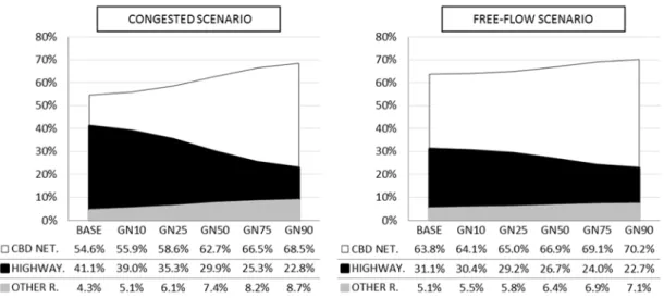
4.2. Results by Road Type
Figure4shows the share by road type of each of the indicators assessed for the base scenarios for congested and free-flow traffic conditions. While the CBD network only carried 14.8% of vehicle-km driven in Madrid and generated 15.7% of the CO2emissions, it represented 63.8% of the air pollution exposure levels in the highly-congested scenario. This is due to the fact that population density in the city center is higher than in the peripheral areas. For the free-flow scenario, similar levels of traffic flow (14.5%) led to a lower share of the PEI_NOxindicator, 54.6%. This is due to the fact that the gross
traffic NOxemission share was higher under congested conditions than under free-flow conditions,
13.3% vs. 10.7%, respectively, in CBD.
Energies 2017, 10, 791 11 of 18
Table 3. Changes in traffic volumes and averages speeds between the SR and the GN highly-congested
scenarios.
Traffic Volume (veh × km) Average Speed (veh × km/veh × hour)
SR GN SR GN
BC 5,884,915 5,884,915 61.0 61.0
Penetration rate (%)
10 −6.9% −3.7% 7.40% −9.8%
25 −17.7% −7.7% 6.80% −19.1%
50 −26.0% −11.3% −14.50% −26.9%
75 −22.8% −12.9% −43.40% −30.7%
90 −15.6% −13.5% −56.20% −32.8%
Notes: BC is the Base case scenario, SR is the Shortest Route scenario, GN is the Green Navigation Scenario.
4.2. Results by Road Type
Figure 4 shows the share by road type of each of the indicators assessed for the base scenarios for congested and free-flow traffic conditions. While the CBD network only carried 14.8% of vehicle-km driven in Madrid and generated 15.7% of the CO2 emissions, it represented 63.8% of the air pollution
exposure levels in the highly-congested scenario. This is due to the fact that population density in the city center is higher than in the peripheral areas. For the free-flow scenario, similar levels of traffic flow (14.5%) led to a lower share of the PEI_NOx indicator, 54.6%. This is due to the fact that the gross traffic NOx emission share was higher under congested conditions than under free-flow conditions, 13.3% vs. 10.7%, respectively, in CBD.
Figure 4. Indicators’ share of the total road network by road type in the base congested and free-flow
scenarios. Notes: CBD NET. stands for Central Business District Network, HIGHWAY. stands for Highways, and OTHER R. stands for Other Roads. Length is the percentage of km of road for each type of road considered, VKM stands for vehicles-km travelled i.e., traffic volume, TEI_CO2 stands for
CO2 traffic emission indicator, TEI_NOx stands for NOx traffic emission indicator, PEI_NOx stands for
population-weighted NOx indicator.
Figure 5 shows the evolution of the PEI_NOx share by road type for the different GN penetration levels considered (rows in the tables below, the sum of the columns add up to 100%). Although for the
free-flow base scenario the CBD share of PEI_NOx was lower than for the congested scenario, it
increased with the penetration rate. Hence, for the highest GN penetration rates (GN75 and GN90), the share of air pollution exposure was similar. This noticeable evolution under free-flow condition was due to the fact that, while NOx gross traffic emissions increased in similar proportion to the congested condition, traffic flows in CBD grew faster as the GN penetration rate increased. Traffic
Figure 4.Indicators’ share of the total road network by road type in the base congested and free-flow scenarios. Notes: CBD NET. stands for Central Business District Network, HIGHWAY. stands for Highways, and OTHER R. stands for Other Roads. Length is the percentage of km of road for each type of road considered, VKM stands for vehicles-km travelled i.e., traffic volume, TEI_CO2stands for CO2traffic emission indicator, TEI_NOxstands for NOxtraffic emission indicator, PEI_NOxstands for
population-weighted NOxindicator.
Figure5shows the evolution of the PEI_NOxshare by road type for the different GN penetration
levels considered (rows in the tables below, the sum of the columns add up to 100%). Although for the free-flow base scenario the CBD share of PEI_NOxwas lower than for the congested scenario,
it increased with the penetration rate. Hence, for the highest GN penetration rates (GN75 and GN90), the share of air pollution exposure was similar. This noticeable evolution under free-flow condition was due to the fact that, while NOxgross traffic emissions increased in similar proportion to the congested
from 14.5% for the free base-case scenario to 22.5%, while NOxgross traffic emissions increased from
11% to 18%. For the congested situation, this growth ranged from 15% to 20% for traffic volumes, and from 13% to 20% for NOxemissions.
flows rose from 14.5% for the free base-case scenario to 22.5%, while NOx gross traffic emissions
increased from 11% to 18%. For the congested situation, this growth ranged from 15% to 20% for
traffic volumes, and from 13% to 20% for NOx emissions.
Figure 5. Evolution of the population exposure to the NOx indicator for different GN penetration rates and road types.
Table 4 shows the variation of traffic performance and environmental indicators by road type (i.e., urban, highway, and extra-urban) for each of the GN penetration rates considered. The impedance function looked for the traffic assignment that minimizes fuel consumption for the entire network. Traffic volumes increased considerably, especially under low-congestion conditions. Travel distances, speed, and congestion had a great influence on traffic emissions [62]. Although the impedance function used also takes the influence of traffic intensity and speed in fuel consumption into account, travel distance was still a major driver of fuel consumption reduction. At the CBD level, all of the indicators worsened with the adoption of eco-routing choices, regardless of the traffic condition considered. Under free-flow conditions, shorter urban routes became even more attractive for green drivers, since road saturation levels were low. Traffic volumes also increased on OTHER roads. However, these growths were compensated by reductions on the highways to obtain a global decrease (Table 2) in the total VKM driven.
Travel times increased noticeably on CBD and OTHER roads. While on CBD roads, there was an increase under highly-congested traffic conditions, and on OTHER peripheral roads, there was a greater increase under free-flow traffic conditions. Nevertheless, travel times on highways significantly decreased as GN penetration rates increases.
In general, GN systems reduced congestion on faster roads (highways) by distributing traffic to shorter, but slower, routes, where saturation rates increase significantly. Therefore, global travel times (Table 2) for the whole region increased. Then GN systems were ineffective at improving traffic performance since congestion was transferred to other areas in the city.
As expected, CO2 emissions also increased at a CBD level and OTHER roads, although this
increase was compensated by the CO2 emission reduction on HIGHWAYS. The greatest impact of
CO2 emissions lies in their contribution to climate change, i.e., in general, no matter where they are
emitted, any emission contributes to global figures, and hence to global warming [18]; therefore, we
can consider GN systems as an effective measure to reduce CO2 emissions, especially when applied
during highly-congested traffic periods.
Figure 5.Evolution of the population exposure to the NOxindicator for different GN penetration rates
and road types.
Table4shows the variation of traffic performance and environmental indicators by road type (i.e., urban, highway, and extra-urban) for each of the GN penetration rates considered. The impedance function looked for the traffic assignment that minimizes fuel consumption for the entire network. Traffic volumes increased considerably, especially under low-congestion conditions. Travel distances, speed, and congestion had a great influence on traffic emissions [62]. Although the impedance function used also takes the influence of traffic intensity and speed in fuel consumption into account, travel distance was still a major driver of fuel consumption reduction. At the CBD level, all of the indicators worsened with the adoption of eco-routing choices, regardless of the traffic condition considered. Under free-flow conditions, shorter urban routes became even more attractive for green drivers, since road saturation levels were low. Traffic volumes also increased on OTHER roads. However, these growths were compensated by reductions on the highways to obtain a global decrease (Table2) in the total VKM driven.
Travel times increased noticeably on CBD and OTHER roads. While on CBD roads, there was an increase under highly-congested traffic conditions, and on OTHER peripheral roads, there was a greater increase under free-flow traffic conditions. Nevertheless, travel times on highways significantly decreased as GN penetration rates increases.
In general, GN systems reduced congestion on faster roads (highways) by distributing traffic to shorter, but slower, routes, where saturation rates increase significantly. Therefore, global travel times (Table2) for the whole region increased. Then GN systems were ineffective at improving traffic performance since congestion was transferred to other areas in the city.
Table 4.Variation of traffic and environmental indicators by road type for each GN penetration rate.
VKM (veh×km) VEH (veh×h) TEI_CO2(kg) TEI_NOx(kg) PEI_NOx(kg×hab/km2)
CBD NET. Cong. Free Cong. Free Cong. Free Cong. Free Cong. Free
BC 870,955 314,411 29,662 7016 141,633 44,528 405 125 6,553,843 2,064,349
GN10 0.1% 0.3% 10.6% 0.6% 2.5% 4.4% 2.0% 4.0% 1.0% 3.3%
GN25 2.8% 7.8% 25.9% 10.6% 8.7% 13.2% 7.8% 13.1% 5.3% 11.7%
GN50 8.2% 20.2% 47.1% 28.1% 18.7% 27.7% 17.2% 28.2% 13.2% 25.2%
GN75 13.5% 31.6% 62.2% 44.9% 27.2% 41.5% 25.3% 42.4% 21.0% 38.1%
GN90 16.4% 37.8% 71.0% 54.5% 31.8% 49.2% 29.6% 50.4% 25.4% 45.2%
HIGHWAY. Cong. Free Cong. Free Cong. Free Cong. Free Cong. Free
BC 3,545,963 1,412,048 45,751 13,622 541,775 222,941 1891 819 3,192,085 1,552,678
GN10 −5.0% −9.3% 2.9% −9.1% −4.1% −5.5% −4.4% −5.6% −1.6% −4.2%
GN25 −11.8% −15.7% 3.4% −14.9% −10.5% −12.3% −11.5% −12.7% −3.0% −10.4%
GN50 −20.9% −25.0% −3.5% −22.3% −19.6% −22.5% −20.8% −23.3% −7.4% −20.8%
GN75 −27.4% −33.4% −11.1% −29.6% −26.4% −31.6% −27.4% −32.8% −13.6% −30.3% GN90 −30.4% −38.1% −14.5% −34.0% −29.7% −36.7% −30.9% −38.2% −16.7% −35.7%
OTHER R. Cong. Free Cong. Free Cong. Free Cong. Free Cong. Free
BC 1,467,996 444,370 21,127 4985 221,394 66,321 751 230 531,349 162,782
GN10 −2.6% 0.7% 9.8% 5.5% −1.7% 6.8% −3.1% 5.4% 6.4% 18.9%
GN25 −4.1% 11.4% 20.6% 26.9% −2.5% 17.7% −5.4% 14.6% 16.4% 47.6%
GN50 0.3% 26.7% 38.6% 58.3% 2.9% 33.1% −1.8% 27.2% 33.2% 87.1%
GN75 6.2% 40.1% 53.9% 85.3% 9.6% 46.7% 3.7% 38.1% 47.6% 115.8%
GN90 9.7% 48.1% 62.9% 102.4% 13.3% 54.9% 6.3% 44.7% 56.4% 131.5%
Notes: CBD NET. stands for Central Business District Network, HIGHWAY. stands for Highways, and OTHER R. stands for Other Roads. BC for Base case scenario, VKM stands for vehicles-km travelled, i.e., traffic volume, VEH stands for vehicles-hour travelled, i.e., travel times, TEI_CO2stands for the CO2traffic emission indicator, TEI_NOx
stands for the NOxtraffic emission indicator, PEI_NOxstands for the population-weighted NOxindicator.
CBD areas are the most populated areas in the region of Madrid. Although for the entire region traffic emissions (both CO2and NOx) decreased, for CBD areas they increased. Although gross NOx
emissions are reduced at a regional level, population exposure levels increased (Table2). Furthermore, population exposure to NOxincreased more quickly on CBD roads than it did for the entire region.
For low GN penetration rates (GN10 to GN50), they increased in similar proportion, yet for GN10, the increase for the entire region is 6.4%, while for CBD roads, it was only 2%. However, for higher GN penetration rates (GN75 and GN90), CBD increased by almost double over the increases in the entire region. Population exposure to air pollution decreased in highways under free-flow traffic and congested conditions for all penetration rates considered.
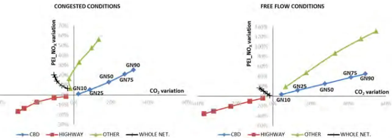
To better understand the impact of this measure on the spatial redistribution of the emissions, Figure6plots TEI_CO2reductions against PEI_NOxreductions by road type. The penetration rate of
green drivers is represented by dots, triangles, squares, or addition signs depending on the type of road being represented. The types of roads are also assigned different colors. Analyzing the results for the entire region (black line), we can consider GN systems as successful for reducing CO2emissions, but ineffective at decreasing local NOxexposure. This is because while the relative increases in CO2 emissions in the CBD were offset by the greater relative decreases in the highways, the relocation of NOx emissions towards the densely populated CBD were not compensated by a reduction in
Figure 6. Impacts of the different levels of GN drivers on the spatial allocation of CO2 emissions and
population exposure to NOx by the road type and traffic situation considered. Percentages on each axis indicate the percent variation in each measure with positive percentages indicating an increase and negative percentages indicating a decrease.
5. Conclusions
A proper environmental assessment of transport policies should take climate change and air pollution co-benefits and conflicts into account. Although this research does not take all the drivers to evaluate population exposure to air pollution into account, weighting emissions by population density reveals important insights. PEI makes emissions produced in dense areas more significant than those produced in less dense areas.
According to the results of this study, GN systems are an effective tool for fighting climate change, but are ineffective at reducing local air pollution, since it increases in highly-populated areas.
These results are consistent under both the congested and free-flow conditions. On the one hand, CO2
emissions reductions increase with the level of penetration of GN drivers. Furthermore, the greatest
CO2 reductions occur in highly-congested scenarios. On the other hand, considering NOx emissions at
the regional level, the results showed a reduction for the Madrid region, but with a spatial reallocation
at the CBD areas. Besides, the results showed an upsurge in the population’s exposure to NOx air
pollution for the whole region. This increase is greater in congested situations than in free-flow situations, and it rises along with the percentage of green drivers.
Traffic performance worsens considerably as eco-routing drivers increase due to the reallocation of traffic to shorter routes. On the one hand, considering the entire network, travel times increase for all GN penetration levels in highly-congested scenarios, and for penetration levels higher than 25% for free-flow situations. On the other hand, although global traffic volumes diminish, congestion increases on CBD and OTHER peripheral roads. Finally, other important urban sustainability factors, such as noise and accidents, create a vulnerable situation for travelers such as pedestrians and cyclists, who are expected to be negatively affected by the increase in traffic volume on CBD roads.
On-board navigation systems need be enhanced to take both traffic performance and traffic emissions into account. There are some advances in this regard, e.g., Jimenez et al. [67] have developed an objective function that optimizes the energy used on the trip, while observing the time schedule. However, the different spatial impact of transport emissions should also be taken into account, in order to efficiently achieve not only greener, but also cleaner cities. Therefore, there is a need to develop navigation algorithms that balance traffic performance, air pollution and climate change impacts to obtain the optimal route, taking the impacts on the entire network into account, instead of focusing on individual fuel consumption reductions.
Acknowledgments: The authors acknowledge the support of the Lee Schipper Memorial Scholarship for Sustainable Transport and Energy Efficiency for the completion of this work. Particularly, the scholar mentors: Måns Lönnroth and Sam Zimmerman. They also acknowledge the support of the ICT-Emissions project 2011-2015, “Development of a methodology and tools for assessing the impact of ICT measures in road transport emissions” EU-FP7 Grant Agreement No. 288568.
Figure 6.Impacts of the different levels of GN drivers on the spatial allocation of CO2emissions and population exposure to NOxby the road type and traffic situation considered. Percentages on each axis
indicate the percent variation in each measure with positive percentages indicating an increase and negative percentages indicating a decrease.
5. Conclusions
A proper environmental assessment of transport policies should take climate change and air pollution co-benefits and conflicts into account. Although this research does not take all the drivers to evaluate population exposure to air pollution into account, weighting emissions by population density reveals important insights. PEI makes emissions produced in dense areas more significant than those produced in less dense areas.
According to the results of this study, GN systems are an effective tool for fighting climate change, but are ineffective at reducing local air pollution, since it increases in highly-populated areas. These results are consistent under both the congested and free-flow conditions. On the one hand, CO2emissions reductions increase with the level of penetration of GN drivers. Furthermore, the greatest CO2reductions occur in highly-congested scenarios. On the other hand, considering NOx
emissions at the regional level, the results showed a reduction for the Madrid region, but with a spatial reallocation at the CBD areas. Besides, the results showed an upsurge in the population’s exposure to NOxair pollution for the whole region. This increase is greater in congested situations than in free-flow
situations, and it rises along with the percentage of green drivers.
Traffic performance worsens considerably as eco-routing drivers increase due to the reallocation of traffic to shorter routes. On the one hand, considering the entire network, travel times increase for all GN penetration levels in highly-congested scenarios, and for penetration levels higher than 25% for free-flow situations. On the other hand, although global traffic volumes diminish, congestion increases on CBD and OTHER peripheral roads. Finally, other important urban sustainability factors, such as noise and accidents, create a vulnerable situation for travelers such as pedestrians and cyclists, who are expected to be negatively affected by the increase in traffic volume on CBD roads.
On-board navigation systems need be enhanced to take both traffic performance and traffic emissions into account. There are some advances in this regard, e.g., Jimenez et al. [67] have developed an objective function that optimizes the energy used on the trip, while observing the time schedule. However, the different spatial impact of transport emissions should also be taken into account, in order to efficiently achieve not only greener, but also cleaner cities. Therefore, there is a need to develop navigation algorithms that balance traffic performance, air pollution and climate change impacts to obtain the optimal route, taking the impacts on the entire network into account, instead of focusing on individual fuel consumption reductions.
“Development of a methodology and tools for assessing the impact of ICT measures in road transport emissions” EU-FP7 Grant Agreement No. 288568.
Author Contributions: Fiamma Perez-Prada conducted the simulations, defined the indicators, analyzed the data, and wrote the manuscript. Andres Monzon directed the research, reviewed the manuscript, and proposed changes and improvements to its structure. Cristina Valdes designed and conducted the simulations and analyzed the data.
Conflicts of Interest:The authors declare no conflict of interest.
References
1. Samaras, Z.; Ntziachirstos, L.; Toffolo, S.; Magra, G.; Garcia-Castro, A.; Valdes, C.; Vock, C.; Maier, W. Quantification of the effect of ITS on CO2 emissions from road transportation.Transp. Res. Procedia2016,14, 3139–3148. [CrossRef]
2. Garcia-Castro, A.; Monzon, A. Using floating car data to analyse the effects of ITS measures and eco-driving.
Sensors2014,14, 21358–21374. [CrossRef] [PubMed]
3. Baptista, P.C.; Azevedo, I.L.; Farias, T.L. ICT solutions in transportation systems: Estimating the benefits and environmental impacts in the Lisbon.Procedia-Soc. Behav. Sci.2012,54, 716–725. [CrossRef]
4. Xia, H.; Boriboonsomsin, K.; Barth, M. Dynamic eco-driving for signalized arterial corridors and its indirect network-wide energy/emissions benefits.J. Intell. Transp. Syst.2013,17, 31–41. [CrossRef]
5. Ericsson, E.; Larsson, H.; Brundell-Freij, K. Optimizing route choice for lowest fuel consumption—Potential effects of a new driver support tool.Transp. Res. Part C Emerg. Technol.2016,14, 369–383. [CrossRef] 6. Ahn, K.; Rakha, H.A. Network-wide impacts of eco-routing strategies: A large-scale case study.Transp. Res.
Part D Transp. Environ.2013,25, 119–130. [CrossRef]
7. Valdes, C.; Perez-Prada, F.; Monzon, A. Eco-routing: More green drivers means more benefits? In Proceedings of the XII Conference on Transport Engineering, Valencia, Spain, 7–9 June 2016.
8. Perez-Prada, F.; Monzon, A. Ex-post environmental and traffic assessment of a speed reduction strategy in Madrid’s inner ring-road.J. Transp. Geogr.2017,58, 256–268. [CrossRef]
9. CO2Emissions from Fuel Combustion 2014, IEA, Paris. Available online:http://dx.doi.org/10.1787/co2_
fuel-2014-en(accessed on 8 June 2017).
10. European Environment Agency.Air Quality in Europe—2012; EEA Report No. 4/2012; European Environment Agency: Copenhagen, Denmark, 2012.
11. Global Report on Human Settlements 2011. Cities and Climate Change. (2011). Available online:
https://unhabitat.org/books/cities-and-climate-change-global-report-on-human-settlements-2011/
(accessed on 8 June 2017).
12. Hickman, R.; Hall, P.; Banister, D. Planning more for sustainable mobility.J. Transp. Geogr.2013,33, 210–219. [CrossRef]
13. Hickman, R.; Ashiru, O.; Banister, D. Transport and climate change: Simulating the options for carbon reduction in London.Transp. Policy2010,17, 110–125. [CrossRef]
14. Banister, D.; Stead, D.; Steen, P.; Akerman, J.; Dreborg, K.; Nijkamp, P.; Schleicher-Tappeser, R.European
Transport Policy and Sustainable Mobility; Routledge (Taylor & Francis Group): Abingdon, UK, 2000.
15. Schipper, L.J.; Fulton, L. Carbon Dioxide Emissions from Transportation: Trends, Driving Factors, and Forces for Change. InHandbook of Transport and the Environment; Hensher, D.A., Button, K.J., Eds.; Emerald Publishing: Bradford, UK, 2003; Volume 4, pp. 203–225.
16. Wright, L.; Fulton, L. Climate Change Mitigation and Transport in Developing Nations.Transp. Rev.2005,25, 691–717. [CrossRef]
17. Rodrigue, J.-P.; Comtois, C.; Slack, B.The Geography of Transport Systems; Routledge: Abingdon, UK, 2009. 18. Health Effects Institute.Traffic-Related Air Pollution: A Critical Review of the Literature on Emissions, Exposure,
and Health Effects; Special Report 17; Health Effects Institute: Boston, MA, USA, 2010.
19. White, R.H.; Spengler, J.D.; Dilwali, K.M.; Barry, B.E.; Samet, J.M. Report of workshop on traffic, health, and infrastructure planning.Arch. Environ. Occup. Health2005,60, 70–76. [CrossRef] [PubMed]
21. Woodcock, J.; Edwards, P.; Armstrong, B.J.; Ashiru, O.; Banister, D.; Beevers, S.; Chalabi, Z.; Chowdhury, Z.; Cohen, A.; Franco, O.H.; et al. Public health benefits of strategies to reduce greenhouse-gas emissions: Urban land transport.Lancet2009,374, 1930–1943. [CrossRef]
22. Thambiran, T.; Diab, R.D. The case for integrated air quality and climate change policies.Environ. Sci. Policy 2011,14, 1008–1017. [CrossRef]
23. Oxley, T.; Elshkaki, A.; Kwiatkowski, L.; Castillo, A.; Scarbrough, T.; ApSimon, H. Pollution abatement from road transport: Cross-sectoral implications, climate co-benefits and behavioural change.Environ. Sci. Policy
2012,19–20, 16–32. [CrossRef]
24. Mao, X.; Yang, S.; Liu, Q.; Tu, J.; Jaccard, M. Achieving CO2emission reduction and the co-benefits of local air pollution abatement in the transportation sector of China.Environ. Sci. Policy2012,21, 1–13. [CrossRef] 25. Geng, Y.; Ma, Z.X.; Xue, B.; Ren, W.X.; Liu, Z.; Fujita, T. Co-benefit evaluation for urban public transportation
sector—a case of Shenyang, China.J. Clean. Prod.2013,58, 82–91. [CrossRef]
26. Xue, X.Z.; Ren, Y.; Cui, S.H.; Lin, J.Y.; Huang, W.; Zhou, J. Integrated analysis of GHGs and public health damage mitigation for developing urban road transportation strategies.Transp. Res. Part D Transp. Environ. 2015,35, 84–103. [CrossRef]
27. Dhar, S.; Shukla, P.R. Low carbon scenarios for transport in India: Co-benefits analysis.Energy Policy2015, 81, 186–198. [CrossRef]
28. Pathak, M.; Shukla, P.R. Co-benefits of low carbon passenger transport actions in Indian cities: Case study of Ahmedabad.Transp. Res. Part D Transp. Environ.2016,44, 303–316. [CrossRef]
29. Schipper, L.; Fulton, L. Disappointed by diesel? Impacts of shift to diesels in Europe through 2006.Transp. Res.
Rec. J. Transp. Res. Board2009,2139, 1–10. [CrossRef]
30. Schipper, L.; Fulton, L. Dazzled by diesel? The impact on carbon dioxide emissions of the shift to diesels in Europe through 2009.Energy Policy2013,54, 3–10. [CrossRef]
31. Leinert, S.; Daly, H.; Hyde, B.; Gallachóir, B.Ó. Co-benefits? Not always: Quantifying the negative effect of a CO2-reducing car taxation policy on NOxemissions.Energy Policy2013,63, 1151–1159. [CrossRef]
32. Panwar, N.L.; Shrirame, H.Y.; Rathore, N.S.; Jindal, S.; Kurchania, A.K. Performance Evaluation of a Diesel Engine Fueled with Methyl Ester of Castor Seed Oil.Appl. Therm. Eng.2010,30, 245–249. [CrossRef] 33. Saravanan, S.; Nagarajan, G.; Rao, G.L.N.; Sampath, S. Combustion characteristics of a stationary diesel
engine fuelled with a blend of crude rice bran oil methyl ester and diesel.Energy2010,35, 94–100. [CrossRef] 34. Qi, D.H.; Chen, H.; Geng, L.M.; Bian, Y.Z.; Ren, X.C. Performance and combustion characteristics of
biodiesel-diesel-methanol blend fuelled engine.Appl. Energy2010,87, 1679–1686. [CrossRef]
35. Lin, C.-Y.; Huang, J.-C. An oxygenating additive for improving the performance and emission characteristics of marine diesel engines.Ocean Eng.2003,30, 1699–1715. [CrossRef]
36. Godiganur, S.; Murthy, C.S.; Reddy, R.P. Performance and emission characteristics of a Kirloskar HA394 diesel engine operated on fish oil methyl esters.Renew. Energy2010,35, 355–359. [CrossRef]
37. Hooftman, N.; Oliveira, L.; Messagie, M.; Coosemans, T.; Van Mierlo, J. Environmental Analysis of petrol, diesel and electric passenger cars in a Belgian urban setting.Energies2016,9, 84. [CrossRef]
38. Sioshansi, R.; Fagiani, R.; Marano, V. Cost and emissions impacts of plug-in hybrid vehicles on the Ohio power system.Energy Policy2010,38, 6703–6712. [CrossRef]
39. Lang, J.; Cheng, S.Y.; Zhou, Y.; Zhao, B.B.; Wang, H.Y.; Zhang, S.J. Energy and environmental implications of hybrid and electric vehicles in China.Energies2013,6, 2663–2685. [CrossRef]
40. Ghafghazi, G.; Hatzopoulou, M. Simulating the air quality impacts of traffic calming schemes in a dense urban neighborhood.Transp. Res. Part D Transp. Environ.2015,35, 11–22. [CrossRef]
41. Jazcilevich, A.; Mares Vázquez, J.M.; Ramírez, P.L.; Pérez, I.R. Economic-environmental analysis of traffic-calming devices.Transp. Res. Part D Transp. Environ.2015,36, 86–95. [CrossRef]
42. Garcia-Castro, A.; Monzon, A.; Valdes, C.; Romana, M. Modelling different penetration rates of eco-driving in urban areas. Impacts on traffic flow and emissions.Int. J. Sustain. Transp.2016,11, 282–294. [CrossRef] 43. Madireddy, M.; de Coense, B.; Can, A.; Degraeuwe, B.; Beusen, B.; de Vilieger, I.; Botteldooren, D. Assessment
of the impact of speed limit reduction and traffic signal coordination on vehicle emissions using an integrated approach.Transp. Res. Part D Transp. Environ.2011,16, 504–508. [CrossRef]
45. Monzon, A.; Pardillo, J.; Vega, L.; Bustinduy, J.; Vicente, A.; Perez, M. El programa de mejoras de la M-30 en el contexto de una estrategia de movilidad sostenible para Madrid.Rev. Obras Publicas. CICCP.2005,N 3454, 7–26.
46. Perez-Prada, F.; Monzon, A. Cuantificación y evaluación de los impactos económicos, sociales y ambientales de calle30, Horizonte 2010. In Proceedings of the Actas del X Congreso de Ingeniería del Transporte: Transporte Innovador y Sostenible de Cara al Siglo XXI, Granda, Spain, 20–22 June 2012.
47. Gonzalez Diez, V.M.; Verner, D.; Corrales, M.E.; Puerta, J.M.; Mendieta Umaña, M.P.; Morales, C.; Suarez, D.; Linares, A.M.; Scholl, L.; Quintanilla, O.; et al.Building Resilience and Reducing Emissions. Climate Change and IDB; Inter-American Development Bank: Washington, DC, USA, 2014.
48. Toffolo, S.; Morello, E.; Samaras, Z.; Ntziachristos, L.; Vock, C.; Maier, W.; Garcia-Castro, A. ICT-emissions methodology for assessing ITS and ICT solutions. In Proceedings of the Transport Research Arena, Paris, France, 14–17 April 2014.
49. VISUM 14.0 Basics. Available online: http://vision-traffic.ptvgroup.com/en-us/products/ptv-visum/
(accessed on 8 June 2017).
50. Han, X.; Naeher, L.P. A review of traffic-related air pollution exposure assessment studies in the developing world.Environ. Int.2015,32, 106–120. [CrossRef] [PubMed]
51. Beckerman, B.; Jerrett, M.; Brook, J.R.; Verma, D.K.; Arain, M.A.; Finkelstein, M.M. Correlation of nitrogen dioxide with other traffic pollutants near a major expressway.Atmos. Environ.2008,42, 275–290. [CrossRef] 52. Laña, I.; Del Ser, J.; Padró, A.; Vélez, M.; Casanova-Mateo, C. The role of local urban traffic and meteorological conditions in air pollution: A data-based case study in Madrid, Spain.Atmos. Environ.2016,145, 424–438. [CrossRef]
53. Gorham, R. Air Pollution from Ground Transportation: An Assessment of Causes, Strategies and Tactics, and Proposed Actions for the International Community. Available online:http://www.un.org/esa/gite/ csd/gorham.pdf(accessed on 8 June 2017).
54. Brown, M.; Sarnat, S.; DeMuth, K.; Brown, L.; Whitlock, D.; Brown, S.; Tolbert, P.; Fitzpatrick, A. Residential proximity to a major roadway is associated with features of asthma control in children.PLoS ONE2012,7, e37044. [CrossRef] [PubMed]
55. Porebski, G.; Wo´zniak, M.; Czarnobilska, E. Residential proximity to major roadways is associated with increased prevalence of allergic respiratory symptoms in children. Ann. Agric. Environ. Med. 2014,21, 760–766. [CrossRef] [PubMed]
56. Monzon, A.; Cascajo, R.; Díaz, M.; Barberán, A.Observatorio de la Movilidad Metropolitana; Informe 2014; Talleres del Centro de Publicaciones del MAGRAMA: Madrid, Spain, 2016.
57. Valdes, C. Optimization of Urban Mobility Measures to Achieve WIN-WIN Strategies. Ph.D. Thesis, Universidad Politecnica de Madrid, Madrid, Spain, 2012.
58. Valdes Serrano, C.; Garcia-Castro, A.; Perez-Prada, F.; Tuffanelli, G.; Cianfano, M.; Magra, G.; Toffollo, S.; Monzón, A. Deliverable 6.2: Field Trials and Simulation Comparison. 2015. Available online: http://www.ict-emissions.eu/wp-content/uploads/2012/05/D_6_2_-Field-trials-and-simulation-comparison_Final_opt.pdf(accessed on 8 June 2017).
59. Direccion General de Sostenibilidad y Planificacion de la Movilidad Ayuntamiento de Madrid. Estudio del Parque Circulante de la Ciudad de Madrid Año 2013. Available online:
http://www.madrid.es/UnidadesDescentralizadas/Sostenibilidad/EspeInf/EnergiayCC/03Energia/ 3bMovilidad/ParqueCirculante/Ficheros/EstudioPCMad2013.pdf(accessed on 8 June 2017).
60. Secciones censales de la Comunidad de Madrid. Madrid Region Government. Available online: http: //www.madrid.org/iestadis/fijas/clasificaciones/seccioncensal.htm(accessed on 8 June 2017).
61. Panis, L.I.; Beckx, C.; Broekx, S.; De Vlieger, I.; Schrooten, L.; Degraeuwe, B.; Pelkmans, L. PM, NOxand CO2 emission reductions from speed management policies in Europe.Transp. Policy2011,18, 32–37. [CrossRef] 62. Grote, M.; Williams, I.; Preston, J.; Kemp, S. Including congestion effects in urban road traffic CO2emissions
modelling: Do Local Government Authorities have the right options?Transp. Res. Part D Transp. Environ. 2016,43, 95–106. [CrossRef]
64. Ahn, K.; Rakha, H. The effects of route choice decisions on vehicle energy consumption and emissions.
Transp. Res. Part D Transp. Environ.2008,13, 151–167. [CrossRef]
65. Minett, C.F.; Salomons, A.M.; Daamen, W.; Van Arem, B.; Kuijpers, S. Eco-routing comparing fuel consumption of different routes between origin and destination using field test speed profiles and synthetic speed profiles. In Proceedings of the Integrated and Sustainable Transportation Systems, Vienna, Austria, 29 June–1 July 2011.
66. Valdes, C. Deliverable 6.3: Results of Application of ICT Measures in ICT-EMISSIONS Partner Cities. 2015. Available online: http://www.ict-emissions.eu/wp-content/uploads/2012/05/D_6_3_Results-of-application-of-ICT-measures_FINAL.pdf(accessed on 8 June 2017).
67. Jiménez, F.; Cabrera-Montiel, W.; Tapia-Fernandz, S. System for road vehicle energy optimization using real time road and traffic information.Energies2014,7, 3576–3598. [CrossRef]