A large displacement structural analysis of a pipeline subjected to gravity and buoyancy forces

(1)

A large displacement structural analysis of a pipeline

subjected to gravity and buoyancy forces

Juan Carlos Mosquera∗_{, Jaime Garc´ıa-Palacios}a_{and Avelino Samart´ın}b

∗_{Assistant Professor. Dept. of Structural Mechanics} ETSICCYP. UPM. Ciudad Universitaria s/n. 28040 Madrid

a_{Assistant Professor. of Civil Engineering: Hydraulic and Energetic, UPM. Madrid} b_{Full Professor. Dept. of Structural Mechanics, UPM. Madrid}

Abstract

A nonlinear analysis of an elastic tube subjected to gravity forces and buoyancy pressure is carried out. An update lagrangian formulation is used. The structural analysis efficiency in terms of computer time and accuracy, has been improved when load stiffness matrices have been introduced. In this way the follower forces characteristics such as their intensity and direction changes can be well represented. A sensitivity study of different involved variables on the final deformed pipeline shape is carried out.

Keywords:Geometrically nonlinear structures, large displacements, follower forces, hydro-static actions

1. Introduction

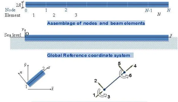
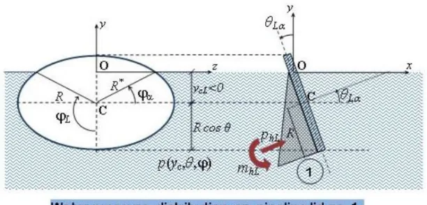
It is considered a pipeline of total lengthLT = N L. For analysis purpose the pipeline is

divided intoN segments of equal lengthL. Each elementiwithi= 1,2, . . . , N is limited by two nodes, 1 and 2, using local numbering andn−1enin global numbering in whichn

varies from 0 toN. The two extreme nodes 0 andN correspond to two lids of weightPLα,

withα= 0andα= 1as it is shown in figure1a.

The circular constant section of the pipeline has an external radiusR. The weight of the tube is represented by a uniform distributed load of intensitypper unit of length. In addition, the tube is floating on the sea and therefore it is subjected to an upward hydrostatic pressure. The sea density isγw. Waves and current forces does not exist. Therefore, it is

(2)

Figure 1: Pipeline discretizaci´on

modulusE, flexural inertiaIzand areaΩ. All loads are modeled in a first approximation as

concentrated at extreme nodes of each pipeline segment.

The objective of this paper is to find the final equilibrated deformed position of the pipeline subjected to the former loads.

The following system of coordinate axes is adopted: General axes Oxyfor load definition, in which the origin O s the intersection of the vertical at initial pipeline section and the horizontal corresponding to the still water level (SWL). The axis Oxis horizontal and the axis Oyis upwards vertical (figure1b). Ii is assumed that inertial forces due to the waves and sea current does not exist. Finally, a local coordinate systems, nis introduced to define the stress-resultants for each pipeline element 12. The origin of these local axes is at node 1 and the axissis the straight line joining the node 1 and 2. The axisnis normal to the axiss. The axess, nrotated in such a way that their directions became parallel to horizontal and vertical, i.e. to the general axes Oxyare designated byx,¯ y¯.

(3)

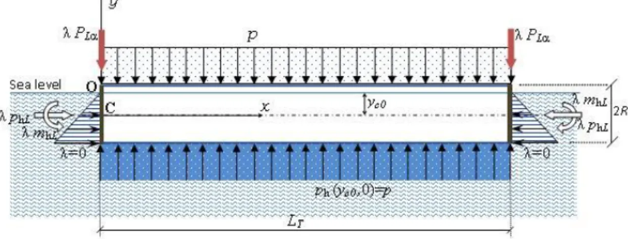
therefore only the distributed loading is acting, i.e. the pipeline weight and the Archimedes uplift pressure. In figure2the horizontal position of equilibrium of the pipeline is shown. The tube is subjected in this position to its weight balanced by the Archimedes uplift. The remaining loads, the lids weight and the hydrostatic pressure on them, are multiplied by a factorλ = 0 i.e. they are not acting on the pipeline yet. From this initial position of equilibrium the loading on the extreme sections of the pipeline are increasing continuously by varying the factorλfrom its initial valueλ = 0to the final oneλ= 1. An incremental analysis technique is used starting at current configuration of equilibriumC1of the deformed tube, that it corresponds to a value0< λ <1. From this position the lids forces are increasing by the factorλ+dλand it is attempting to find the new target configuration of equilibriumC2 corresponding to these incremental loads. It should be noted that the weight of the pipeline remains constant, both in intensity as in direction, along the length of the tube. Moreover, the Archimedes pressure along the pipeline is not affected by this factor incrementdλ, but due to its follower characteristic attached to the structure, according the classification given in [2], its intensity and direction vary because they are dependent of the deformed geometry of the pipeline. These follower loads not only change its direction due to the incremental rotations occurring at the tube sections along the pipeline, but also its intensity caused by the incremental displacements produced along the pipeline.

Figure 2: Initial configuraci´onC0of the tube in equilibrium

This paper is structured as follows. First, it is studied the hydrostatic pressure on a pipeline slice and its incremental changes when the slice undergoes a differential rotation

(4)

iteratively until a final equilibrium position at the end of step loadλ+dλis reached. In these equations the appearance of load stiffness matrices due to the follower loads. By an incre-mental procedure or a step by step technique the final equilibrium position of the pipeline, i.e. the pipeline position corresponding to the final value of the load factorλ= 1can be found. It was found that the inclusion in the analysis of these load matrices allows greater computa-tional efficiency and a better accuracy in the results. Several application examples are shown and in some of them a sensitivity analysis of some key variables illustrate the computational techniques developed. Finally the paper is closed with some general conclusions.

2. Distribution and resultant of the pressure loading on a

tube slice

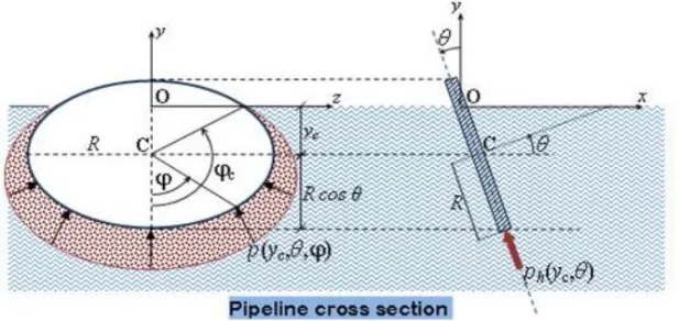
It is assumed a pipeline slice inclined respect to horizontal an angleθ. In figure3the hydro-static pressure distribution on a semi-submerged cross-section of the pipeline is shown. This pressurep(yc, θ, ϕ)is function of following variables: the ordinateycof the center of the

cir-cle, the slopeθof the section respect to the vertical plane and the position of the application point of the pressure defined by the angleϕ. The resultant force,ph(yc, θ)ds, of this pressure

distribution on a pipeline slice of thicknessdsis contained in its middle plane.

Figure 3: Pressure distribution on a circular section

In the following the expressions of the pressure distributionp(yc, θ, ϕ)and its resultant

ph(yc, θ)dsas function of the position of the tube center measured by the ordinate yc are

(5)

• Slice in the airyc≥Rcosθ

p(yc, θ, ϕ) = 0 (1)

ph(yc, θ) = 0 (2)

• Semi-submerged sliceRcosθ≥yc≥ −Rcosθ

p(yc, θ, ϕ) =γw[Rcosθcosϕ−yc] (3)

with ϕc≥ϕ≥ −ϕc and ϕc= arctan

³ _y

c

Rcosθ

´

ph(yc, θ) = 2 Z _ϕ_c

0

p(yc, θ, ϕ) cosϕRdϕ=

γwR2 "

arccos³ yc

Rcosθ

´

− yc

Rcosθ

r

1−³ yc

Rcosθ

´2#

(4)

• Submerged slice−Rcosθ≥yc

p(yc, θ, ϕ) =γw(Rcosθcosϕ−yc) with −π≥ϕ≥π (5)

ph(yc, θ) = 2 Z π

0

p(yc, θ, ϕ) cosϕRdϕ=γwπR2cos2θ (6)

The variation of the pressure resultant caused by a modification of the position of the grav-ity center of the slice defined by an infinitesimal vertical displacementv0and an infinitesimal rotationθ0are found by the expression:

dpt(yc, θ) = ∂ph(yc, θ)

∂yc

v0+∂ph(yc, θ)

∂θ θ0

in which ∂ph(yc,θ)

∂yc and

∂ph(yc,θ)

(6)

fol-lows:

Slice in the airyc ≥Rcosθ

∂ph(yc, θ)

∂yc = 0 (7)

∂ph(yc, θ)

∂θ = 0 (8)

Semi-submerged sliceRcosθ≥yc≥ −Rcosθ

∂ph(yc, θ)

∂yc =−2γwRcosθ r

1−³ yc

Rcosθ

´2

(9)

∂ph(yc, θ)

∂θ =−2γwR

2_cos_θ_sin_θ_arccos³ yc

Rcosθ

´

(10)

Submerged slice−Rcosθ≥yc

∂ph(yc, θ)

∂yc = 0 (11)

∂ph(yc, θ)

∂θ =−2γwπR

2_cos_θ_sin_θ ₍₁₂₎

3. Equivalent loads at element nodes

3..1. Analysis procedure

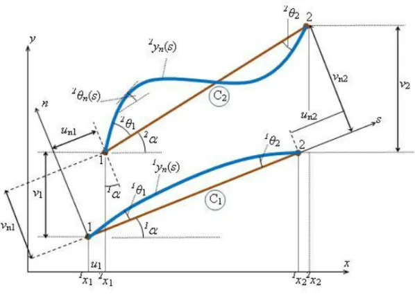
The analysis of the pipeline structure is carried out according to an incremental procedure, eventually iterative within load steps. That means, the final position of the pipeline is reached by successive finite increments of the loaddλ, starting at the value λ = 0and increasing until the final load valueλ= 1. The analysis is described according to an updated lagrangian formulation (UL), in which in each load step the equilibrate configurationC1is known and the adopted local coordinate axis for referencesandnare attached to the known configuration

C1as it is shown in figure4. The axissjoints nodes 1 and 2 of element and the normal axis

ncorresponds to an anticlockwise rotation ofπ

2 of the axiss.

3..2. Displacement independent loads

The load of this type acting on the pipeline is the weight and it is assumed this constant load is applied to a beam element of lengthL inclined an angle α respect to horizontal. The equivalent nodal forces to the weight loading arep = (px1, py1, mz1, px2, py2, mz2)T

at nodes 1 and 2 and they can be approximately expressed in axesx,¯ y¯by means of this formulae:

pxi=pticosα−pnisinα= 0 i= 1,2 (13)

pyi=ptisinα+pnicosα=pL

2 i= 1,2 (14)

(7)

in which

pti= Z L

0

N1

ipds, i= 1,2 (16)

pn1= Z _L

0

N3

1pds, mn1= Z _L

0

N3

2pds (17)

pn2= Z _L

0

N33pds, mn2= Z _L

0

N43pds (18)

In the former expressions the interpolation linear functions have been designed byN1

i =

N1

i(s)withi= 1,2andNi3=Ni3(s)withi= 1,2,3,4are the cubic interpolation functions

of Hermite. They are defined by the expressions:

N11= 1−ξ, N21=ξ (19)

N3

1 = 1−3ξ2+ 2ξ3, N33= 3ξ2−2ξ3 (20)

N3

2 =1Lξ(1−ξ)2, N43=1L(ξ3−ξ2) (21)

withξ= ₁s

L.

The formulae (16)-(18) are valid only in a linear analysis, however their use in a nonlinear analysis can be acceptable if the beam element lengthLis small in comparison to the total pipeline length. In the contrary case, the distributed loading on the beam element should be taken into account in the expression of the nonlinear stiffness matrix of the element. Then the expression (72) of this matrix, given later, should be modified and to include terms related to the the distributed forcep.

3..3. Follower forces

In the case of follower forces the deformed structure should be taken into account in the analysis. This fact leads to the concept of load stiffness matrix. To this end it is assumed, according to an updated lagrangian formulation, that the equilibrated configuration is known

C1. From this known configuration it is arrived to configurationC2when unknown displace-mentsu(s),v(s)andθ(s)are produced due to a load increment. These displacements are expressed in the local coordinates of the elementsandn.

The geometry of the deformed tube element in the configurationC1referred to the local exes can be written if the rotations1_θ

1and1θ2at nodes 1 and 2 are known, as follows: 1_y

n(ξ) =N23(ξ)1θ1+N43(ξ)1θ2 with ξ= ₁s

L (22)

where1_L₌p₍1_x

2−1x1)2+ (1y2−1y1)2.

The rotation variation along the deformed beam element is

1_θ

n(ξ) =

d1_y

n(ξ)

ds = dN3

2(ξ)

ds

1_θ 1+

dN3 4(ξ)

ds

1_θ

(8)

Figure 4: Large displacements in a beam element

If(1_x

i,1yi), withi= 1,2, are the general coordinates of the element nodes then the deformed

elementC1in referred to the general axes is:

1_y₍_ξ_{) =}1_y

1+1Lξsin1α+1yn(ξ) cos1α, 1θ(ξ) =1θn(ξ) +1α (24)

with1_α_{= arctan(}1_y

2−1y1)(1x2−1x1)−1. The resultant pressure 1_p

h(ξ) on the slice ξ, noting yc(ξ) = y(ξ), can be expressed according to section2.:

1_p

h(ξ) =1ph[1yc(ξ),1θ(ξ)] =1ph[1y(ξ),1θ(ξ)] (25)

and the local components of this pressure referred to axessandnare

1_p

hs(ξ) =−1ph(ξ) sin1θ and 1phn(ξ) =1ph(ξ) cos1θ (26)

The displacementsun(ξ),vn(ξ)andθn(ξ)of the former slice leads this slice from the

(9)

are:

un(ξ) = X

i=1,2

uniNi1(ξ) (27)

vn(ξ) = X

i=1,3

vniNi3(ξ) + X

i=2,4

θniNi3(ξ) (28)

θn(ξ) = X

i=1,3

vnidN

3

i(ξ)

ds +

X

i=2,4

θnidN

3

i(ξ)

ds (29)

whereuni,vniandθniare the unknown displacements of nodeireferred to the element local

axes in configurationC1_.

The equations of the deformed tube element in the configurationC2expressed in local coordinates,sandn, are:

2_x

n(ξ) =un(ξ), 2yn(ξ) =1yn+vn(ξ), and 2θn(ξ) =1θn(ξ) +θn(ξ) (30)

which referred to the general axes became:

2_x₍_ξ_{) =}1_x₍_ξ_{) +}_u

n(ξ) cos1α−1vn(ξ) sin1α=1x(ξ) +u(ξ) (31)

2_y₍_ξ_{) =}1_y₍_ξ_{) +}_u

n(ξ) sin1α+1vn(ξ) cos1α=1y(ξ) +v(ξ) (32)

2_θ₍_ξ_{) =}1_θ₍_ξ_{) +}_θ

n(ξ) (33)

The hydrostatic pressure resultant2_p

h(ξ)on the sliceξin the configurationC2is now modi-fied to the following value:

2_p

h(ξ) =1ph[2x(ξ),2y(ξ),2θ(ξ)] =1ph[2x(ξ)] (34)

withx(ξ) = [2_x₍_ξ₎_,2_y₍_ξ₎_,2_θ₍_ξ_{)]. These pressure components}2_p

hs(ξ)and2phn(ξ)referred

to local axessandnare respectively:

2_p

hs(ξ) =−1ph[2x(ξ),2y(ξ),2θ(ξ)] sin2θn(ξ)

=−1_p

h[2x(ξ)] sin[1θn(ξ) +θn(ξ)] (35)

2_p

hn(ξ) =1ph[2x(ξ),2y(ξ),2θ(ξ)] cos2θn(ξ)

=−1ph[2x(ξ)] cos[1θn(ξ) +θn(ξ)] (36)

In order to find the resultant pressure,ph(ξ), variation in the sliceξproduced when the slice

changes from configurationC1toC2is necessary to compute the difference2ph(ξ)−1ph(ξ).

This difference can be expressed in a Taylor expansion in the neighborhood1_p

h(ξ). Taking

into account (31), (32) and (33) the following expression is obtained:

2_p

h[2x(ξ)] =1ph[1x(ξ)] +A(ξ)

∂1_p

h

∂yc

+B(ξ)∂1ph

(10)

where

A(ξ) = sin1_αX

i=1,2

uniNi1(ξ) + cos1α 

X

i=1,2

vniN23i−1(ξ) + X

i=1,2

θniN23i(ξ) 



B(ξ) = X

i=1,2

vni

dN3 2i−1(ξ)

dξ +

X

i=1,2

θnidN

3 2i(ξ)

dξ

and therefore resultant pressure components in local exes are:

2_p

hs(ξ) =−1ph[2x(ξ)] sin(1θn+θn) =−1ph[2x(ξ)] sin1θn−1ph[2x(ξ)]θncos1θn

=1_p

hs[1x(ξ)]−sin1θn ·

A(ξ)∂1ph

∂yc

+B(ξ)∂1ph

∂θ

¸ −1_p

hn[1x(ξ)]B(ξ)

2_p

hn(ξ) =1ph[2x(ξ)] cos(1θn+θn) =1ph[2x(ξ)] cos1θn−1ph[2x(ξ)]θnsin1θn

=1_p

hn[1x(ξ)] + cos1θn ·

A(ξ)∂ 1_p

h

∂yc +B(ξ)

∂1_p

h

∂θ

¸ +1_p

hs[1x(ξ)]B(ξ)

The load increments2_p

h(ξ)−1ph(ξ)caused by the element displacement from

configura-tionC1toC2are substituted by the following equivalent nodal forcesp= (phsi, phni, phmi)

at element nodesi= 1,2, according to the following expressions in local axes:

phsi=1L Z 1

0

N1

i £₂

phs−1phs ¤

dξ with i= 1,2 (38)

phn1=1L Z 1

0

N3 1

£₂

phn−1phn ¤

dξ, phm1=1L Z 1

0

N3 2

£₂

phn−1phn ¤

dξ (39)

phn2=1L Z 1

0

N33 £₂

phn−1phn ¤

dξ, phm2=1L Z 1

0

N43 £₂

phn−1phn ¤

dξ (40)

3..4. Load stiffness matrices

The follower forces produce equivalent nodal forces that can be represented as stiffness ma-trices. In the following the variation of the follower forces from configurationC1 toC2is expressed in this more convenient way. With this purpose the functionsA(ξ)andB(ξ)are written in matrix form

A(ξ) =a(ξ)dn, B(ξ) =b(ξ)dn (41) wheredn= (dn1,dn2)T is a vector of dimension6×1partitioned in the submatricesdni= (uni, vni, θni)T of dimension3×1with(i= 1,2)and

a(ξ) = [a1(ξ),a2(ξ)], ai(ξ) = [sin1αNi1,cos1αN23i−1,cos1αN23i]

b(ξ) = [b1(ξ),b2(ξ)], bi(ξ) = [0,dN

3 2i−1

dξ , dN3

2i

(11)

The components of the unbalanced resultant total pressure∆ph(ξ) =2ph(ξ)−1ph(ξ)at

sectionξcan be written as follows

2_p

hs−1phs=−sin1θn ·

a(ξ)∂ 1_p

h

∂yc +b(ξ)

∂1_p

h

∂θ

¸

dn−1_p

hcos1θnb(ξ)dn (42)

2_p

hn−1phn= cos1θn ·

a(ξ)∂ 1_p

h

∂yc +b(ξ)

∂1_p

h

∂θ

¸

dn−1phsin1θnb(ξ)dn (43)

These components unbalanced forces ∆phs(ξ) = 2phs(ξ)−1phs(ξ)and∆phn(ξ) =

2_p

hn(ξ)−1phn(ξ)are replaced by the equivalent nodal forcesphsi,phniandphmiat nodes

i,(i = 1,2)of the pipeline element, that are referred to the local axes and their values are computed according to the expressions (39), (38) and (40). The final results are then1

phsi=1L Z 1

0

N1

i∆phs(ξ)dξ=kL1jdn+kL2jdn with i= 1,2 (44) wherej= 1 if i= 1; j= 4 if i= 2

phni=1L Z 1

0

N3

i∆phn(ξ)dξ =kL1jdn+kL2jdn with i= 1,3 (45)

wherej= 2 if i= 1; j= 5 if i= 3

phmi=1L Z 1

0

N3

i∆phn(ξ)dξ=kL1jdn+kL2jdn with i= 2,4 (46)

wherej= 3 if i= 2; j= 6 if i= 4

(47)

The first row vectorskL1jare coming from the integration of terms of the following type

kL1j=±1L Z ₁

0

N_i(1,3)

µ sin1_θ

n

cos1_θ

n ¶ ·

a(ξ)∂ 1_p

h

∂yc +b(ξ)

∂1_p

h

∂θ

¸

dξ (48)

and they correspond to the variation of the intensity of the follower forces. The second row vectorskL2jare obtained as a consequences of the integration terms

kL2j=±1L Z ₁

0

N_i(1,3)1_p

h µ

sin1_θ

n

cos1_θ

n ¶

b(ξ)dξ (49)

and in this case they correspond to the variation of the direction of the follower force. The load stiffness matrices kL1 andkL2 relate the force vectors at nodes to the corre-sponding displacements and they can written

p_n=kL1dn+kL2dn=kLdn (50)

1_{It is usual to distinguish between the load matrices of de dimension}₆_×₆_{the matrices}_kL

1generated by an increment of differential vertical displacementycand the matriceskL2produced by un angle changeθof the section of application of the load pressure. The former load matriceskL1andkL2are partitioned in row matricesj,kL1j

(12)

where

pn = ·

pn1

pn2 ¸

,dn = ·

dn1

dn2 ¸

,kLj =         kLj1 kLj2 kLj3 kLj4 kLj5 kLj6        

(j= 1,2)

where la matrizkLis partitioned as follows ·

p_n₁ pn2

¸ =

·

kL11 kL12

kL21 kL22 ¸ ·

dn1

dn2 ¸

Finally, the expressions of these matrices in general axes are modified by means of suit-able axes transformations. In this way the following final expressions are found

P=KLD, i.e. · P1 P2 ¸ = ·

KL11 KL12

KL21 KL22 ¸ · D1 D2 ¸ (51) where

Pi= (pxi, pyi, mzi)T, Di= (dxi, dyi, θzi)T

These vectors are related to the former vectors expressed in local axes by the transformation formulae

Pi=Tpni, Di=TTdni KLαβ=TkLαβTT

where

T= 

 cos

1_α ₋_sin1_α ₀ sin1_α _cos1_α ₀

0 0 1





¿From a computational point of view it is convenient to use the matrices as functions of the typekL =kL(yc1, yc2,1α)andp=p(yc1, yc2,1α).

4. Pressure resultante on the pipeline lids

Similarly to the section2.the loads on the two extreme sections or lids of the pipeline are studied. En particular the force and moment resultants of the pressure distribution on each of these extreme sections are obtained.

The force resultant,pα

hLand the momentmαhL of the pressure distribution acting at

(13)

Figure 5: Pressure distribution on the end section of the pipeline

angleθLαof the tube, are carried out. This inclination angle respect to the horizontal or slope

at each tube end section is in general different to each end pipeline sectionα. The following results for the forcepα

hLand the momentmαhL pressure resultants on the

pipeline end sectionα:

Section in the air ycLα≥RextcosθLα (52)

pαhL= 0

mα hL= 0

Semi-submerged section RextcosθLα≥ycLα≥ −RextcosθLα (53)

pα

hL=ε2γwR2ext "

ycLα

2 Ã

ϕα+ sinϕαcosϕα+

π

2 !

−Rextcos

3_ϕ

α

3 #

mαhL=ε2γwR3ext "

−ycLαcos

3_ϕ

α

3 +

Rext

16 (2ϕα−sin 2ϕαcos 2ϕα+π) #

Submerged section ycLα≤ −RextcosθLα (54)

pα

hL=εγwπR2extycLα

mα hL=ε

1 3γwπR

4

ext

where

sinϕα=−

ycLα

RextcosθLα

and ε= (−1)α ₍₅₅₎

The occurrence of small variations,v0andθ0, of the depthycLαand rotationθLα

respec-tively, of sectionα, the increment of the resultant pressure forcepα

(14)

are given by the formulae

∆pαhL=

∂pα hL

∂ycLαv0+

∂pα hL

∂θαθ0 and ∆m

α hL=

∂mα hL

∂ycLαv0+

∂mα hL

∂θα θ0 (56)

The expressions of the derivatives ∂pαhL

∂ycLα,

∂mα hL

∂ycLα dep

α

hL andmαhL respect toycLα are

obtained as follows:

∂pα hL

∂ycLα

= 0

∂mα hL

∂ycLα = 0

∂pα hL

∂ycLα =ε2γwR

2

ext "

1 2 ³

ϕα+ sinϕαcosϕα+π

2 ´

+

(yhLαcos2ϕα+Rextcos2ϕαsinϕα)

∂ϕα

∂ycLα #

∂mα hL

∂ycLα =ε2γwR

3

ext "

−cos

3_ϕ

α

3 + (ycLαcos 2_ϕ

αsinϕα+Rextsin2ϕαcos2ϕα)

∂ϕα

∂ycLα #

∂pα hL

∂ycLα =εγwπR

2

ext

∂mα hL

∂ycLα

= 0

where

∂ϕα

∂ycLα=−

1

RextcosθLα

1 p

1−sin2_ϕ

α

(15)

The derivatives∂pαhL

∂θLα,

∂mα hL

∂θLα de∂p

α

hLand∂mαhLrespect toθLαare respectively:

∂pα hL ∂θLα = 0 ∂mα hL ∂θLα = 0

∂pα hL

∂θLα =ε2γwR

2

ext "

(ycLαcos2ϕα+Rextcos2ϕαsinϕα)

∂ϕα

∂θLα #

∂mα hL

∂θLα =ε2γwR

3

ext "

(ycLαcos2ϕαsinϕα+Rextsin2ϕαcos2ϕα)

∂ϕα

∂θLα #

∂pα hL

∂θLα = 0

∂mα hL

∂θLα = 0

where

∂ϕα

∂θLα

=− ycLα

Rextcos2θLα

sinθLα (64)

The two groups of former expressions of the derivatives of the pressure follower forces on the lids of the pipeline represent two elastic springs attached to the pipeline extreme sections

α. One of them elastically restrained the end section displacement and the another the end section rotation. From the computational point of view it is convenient to express the analysis in general coordinates by means the following transformation formulae:

∆pαhLx= ∆pαhLcosθLα= µ

∂pα hL

∂ycLαv0+

∂pα hL

∂θLαθ0 ¶

cosθLα (65)

∆pα

hLy = ∆pαhLsinθLα= µ

∂pα hL

∂ycLα

v0+

∂pα hL

∂θLα

θ0 ¶

sinθLα (66)

∆mα

hLz= ∆mαhL=

∂mα hL

∂ycLαv0+

∂mα hL

∂θα θ0 (67)

These equations can be written in the compact form

∆pαhL=kαhLdαhL with kαhL=         0 ∂p α hL ∂ycLα

cosθLα

∂pα hL

∂θLα

cosθLα

0 ∂p

α hL

∂ycLα

sinθLα

∂pα hL

∂θLα

sinθLα

(16)

and where the force and displacement vector at pipeline end sectionsα= 0,1are defined as follows:

∆pα

hL= [∆pαhLx,∆pαhLy,∆mαLz]T and dαhL= [dαx, dαy, θα]T

Similarly the load vector acting at pipeline end sectionαis defined as

pα

hL= [pαhLx, pαhLy, mαLx]T

5. Stiffness matrix of an element

In addition to the the load stiffness matrices obtained in the previous section the nonlinear stiffness matrix of each beam element of pipeline should be computed. With this objective the incremental equilibrium equations between configurationsC1andC2are formulated and they are discretized by means of the FE method. The obtained results assuming all loads,

Fi = (Fxi, Fyi, Mzi)T, (i = 1,2), are applied at end nodes i, i = 1,2, can be written

according to [3], [1], en forma matricial como sigue: £₁

kl+1_kg¤_d₌2_f₋1_f ₍₆₉₎

withklandkg the linear and the geometric stiffness matrix of a 2-D beam element respec-tively. The displacement increments produced by the change of configuration fromC1toC2 caused by the the increasing of the external loads,2_f₋1_f_{, are collected in the vector}

d= ·

d1

d2 ¸

and the forces are k_f₌ · _k

f1

k_f

2 ¸

(70)

withdi = (dxi, dyi, θi)the displacement increments of node i (i = 1,2). The applied

external loads arek_fi_{= (}k_F

xi,kFyi,kMzi)T withk= 1,2andi= 1,2

The expression of the linear stiffness matrix is:

kl= 

      

EΩ

L 0 0 −ELΩ 0 0

0 12EIz

L3 6EI_L2z 0 −12EI_L3z 6EI_L2z

0 6EIz

L2 4EI_Lz 0 −6EI_L2z 2EI_Lz −EΩ

L 0 0 ELΩ 0 0

0 −12EIz

L3 −6EI_L2z 0 12EI_L3z −6EI_L2z

0 6EIz

L2 2EI_Lz 0 −6EI_L2z 4EI_Lz 

      

(71)

withΩthe area of the resistant cross-section of the beam andIzis the moment of inertial of

the cross-section about the axisz. The geometric stiffness matrix is

kg= ·

kg11 kg12

kg21 kg22 ¸

(17)

where

kg11=   

Fx2

L 0 −MLz1

0 6

5

Fx2(ΩL2+10Iz)

ΩL3 ₁₀1

Fx2(ΩL2+60Iz)

ΩL2 −Mz1

L 101

Fx2(ΩL2+60Iz)

ΩL2 ₁₅2

Fx2(ΩL2+30Iz)

ΩL

 

 (73)

kg12= 

 

−Fx2

L 0 −MLz2

0 −6

5

Fx2(ΩL2+10Iz)

ΩL3 ₁₀1

Fx2(ΩL2+60Iz)

ΩL2 Mz1

L −101

Fx2(ΩL2+60Iz)

ΩL2 ₃₀1

Fx2(−ΩL2+60Iz)

ΩL





=kTg21 (74)

kg22=   

Fx2

L 0

Mz2 L

0 6₅Fx2(ΩL2+10Iz)

ΩL3 −₁₀1

Fx2(ΩL2+60Iz)

ΩL2 Mz2

L −101

Fx2(ΩL2+60Iz)

ΩL2 ₁₅2

Fx2(ΩL2+30Iz)

ΩL

 

 (75)

It is noticed that the former stiffness matrices,klandkg, are symmetric as correspond to a conservative (adjoint) problem.

In the former results is was assumed that the only loads applied on the element are the ones acting at its end nodes, i.e.Fi= (Fxi, Fyi, Mzi)T,(i= 1,2). Then the stress-resultants

at sectionξof the element produced by the loads acting directly on the element span (weight and hydrostatic pressure) must be added the stress-resultants corresponding to the loadsFi:

Fx=Fx1=−Fx2, Fy=−Mz1+Mz2

L , Mz=−Mz1(1−ξ) +Mz2ξ (76)

The equations (76) represent the stress-resultants at sectionξas function of the reactions of the beam element at its end nodes. They have been obtained using the static equilibrium of the beam element.

6. Incremental equilibrium equations of the pipeline

The initial configurationC0 of the pipeline without initial stresses corresponds to the tube subjected only to the uniforme distributed loads of weightpand uplift hydrostatic pressure

ph(yc, θ). The equilibrium position corresponds to the pipeline floating horizontally,θ= 0,

at depthyc defined as the solution of the equationph(yc, θ = 0) = p. The loads due to

the horizontal pressure on lidsp_hLand to the weightPLof the pipeline extreme section, i.e. to the lids, are monotonically introduced from this equilibrium position by means a factorλ

varying from 0 up to 1.

(18)

are known

Loading: p, 1_p

hi(ξ) (i= 1,2, . . . , N), λPLα(α= 0,1), λ1pαhL (77)

Equivalent nodal forces: 1_Fj

i,(i= 1,2) (j= 1,2, . . . , N) (78)

deflections and rotations: 1_xj

i,1yij,1θji, (i= 1,2) (j= 1,2, . . . , N) (79)

Stres-resultants: 1Fxj(ξ),1Fyj(ξ),1Mzj(ξ),(j= 1,2, . . . , N) (80)

If the following load increments,dλPLαanddλ1pαhL, are introduced on the end sections of

the pipeline,α= 0,1, then the pipeline experiments the displacementsdj_i at nodesi= 1,2 of all elementsj. The matrix equation of equilibrium can be written

KD=P (81)

where

K=X

α

[kα

l +kαg −kαL1−kαL2]D+λ X

α=0,1

kα

hLdαhL=dλ X

α=0,1

[p_hL+PLα]

andPLα=PLα[0,−1,0]T is the vector of gravitational loads concentrated at sectionα. The

summations correspond to boolean sums or assembly of all element matrices and vectors of the structural elements. In this way the whole global structure matrices and vector can be built.

The solution of the system of simultaneous linear equations represented by the matrix equation (81) can be carried our by a direct numerical solution method and the displacement vectorDexpressed in global exes is obtained. It is possible to increase the solution accuracy by iterative procedure within the current load step.

Once the displacements are know in the load step it is possible to define all the variables of interest for the configurationC2. These variables should be changed by transforming them to the new coordinate system defined by the achieved configurationC2, i.e. a coordinate transformation should be performed in order to change the already known configurationC2 into the new configurationC1for the new load step.

7. Examples

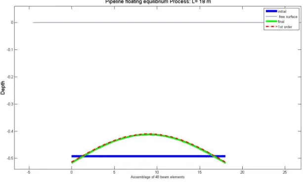
7..1. Symmetric pipeline

In order to illustrate the described analysis a simple example will be presented. The following data of a symmetric pipeline, i.e. with equal lids will be considered: Length: 18 m,Inner radius: 0,945 m, External radius: 1 m

Young modulus: 2×105_kN_/_m2,_{Specific weight}_{: 77 kN}_/_m3,_{Water specific weight}_{: 10,29} kN/m3

The two pipeline lids are equal with thickness 6 cm and weight 14,516 kN each. The total tube weight, lids no included, is: 465,85 kN

(19)

Figure 6: Symmetric pipeline

In figure6 the deformed pipeline obtained by a linear analysis is shown. Also the de-formed pipeline found according to a more elaborated analysis, namely, a nonlinear analysis using an incremental and iterative procedure is presented in the figure. It can be observed that the first order analysis produces larger displacements than the nonlinear analysis.

The initial equilibrated position of the tube (tube weight without lids and uplift Archimedes pressure) is reached for a axis pipeline position of -0,4929 meters.

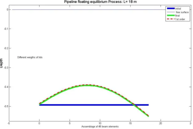
7..2. Nonsymmetric pipeline

The tube used in this example corresponds to the previous tube but with different lid thick-nesses. One lid has 6 cm of thickness and the other 9 cm. The results are shown in figure 7

8. Conclusions

(20)

Figure 7: Nonsymmetric pipeline

9. Acknowledgments

The financial support for this work provided by theDirecci´on General de Investigaci´onof the Spanish Ministry of Education and Science under the research contract DPI2005-09203-02 is grateful recognized by the authors.

References

[1] Garc´ıa-Palacios, J. and Samart´ın, A. and Negro, V. A nonlinear analysis of laying a floating pipeline on the seabed.Engineering Structures, 31(5):1120–1131, 2009.

[2] Schweizerhof, K. and Ramm, E. Displacement dependent pressure loads in nonlinear finite element analisys.Computer and Structures, 18(1):1099–1114, 1984.