GOAL-ORIENTED SELF-ADAPTIVE HP-STRATEGIES FOR FINITE ELEMENT ANALYSIS OF ELECTROMAG-NETIC SCATTERING AND RADIATION PROBLEMS
I. Gomez-Revuelto1, L. E. Garcia-Castillo2, *, and M. Salazar-Palma2
1Dpto. Ingenier´ıa Audiovisual y Com., Universidad Polit´ecnica de
Madrid, E.U.I.T.T Ctra. Valencia Km. 7, Madrid 28031, Spain
2Dpto. Teor´ıa de la Se˜nal y Com., Universidad Carlos III de Madrid,
Escuela Polit´ecnica Superior, Avda. de la Universidad, 30, Legan´es 28911, Madrid, Spain
Abstract—In this paper, a fully automatic goal-orientedhp-adaptive finite element strategy for open region electromagnetic problems (radiation and scattering) is presented. The methodology leads to exponential rates of convergence in terms of an upper bound of an user-prescribed quantity of interest. Thus, the adaptivity may be guided to provide an optimal error, not globally for the field in the whole finite element domain, but for specific parameters of engineering interest. For instance, the error on the numerical computation of theS-parameters of an antenna array, the field radiated by an antenna, or the Radar Cross Section on given directions, can be minimized. The efficiency of the approach is illustrated with several numerical simulations with two dimensional problem domains. Results include the comparison with the previously developed energy-norm basedhp-adaptivity.
1. INTRODUCTION
The use of “adapted” meshes [1], not only to the geometry of the problem domain, but to the solution of the problem itself, is a powerful feature of the Finite Element Method (FEM) [2–5]. When the adaption of the mesh to the solution is done automatically, it is referred to as automatic adaptivity or self-adaptive mesh refinement. There are several types of adaptivity. One of the most powerful type of adaptivity
Received 16 December 2011, Accepted 21 February 2012, Scheduled 7 March 2012
is the so calledhp-adaptivity in which the hrefinements (modification of element size) and the p-refinements (variation of the polynomial order p) are performed simultaneously, providing exponential rates of convergence, even in the presence of singularities. In contrast, only algebraic rates of convergence are (in general) obtained with h
and p schemes. It is worth noting that remeshing techniques [6] are not considered here. Thus, very accurate solutions can be obtained with an hp-adaptive strategy, even in the presence of singularities. Equivalently, approximate solutions within engineering accuracy can be obtained using a minimum number of unknowns.
Several hp-adaptive strategies have appeared in the literature. An extensive comparison in the context of elliptic partial differential equations using triangles can be found in [7]. Most of the strategies reported are h+p methods rather than hp methods, i.e., adaptive methods in which in one step of the adaptivity onlyh, orp, refinements (but not both) are performed. The decision betweenhorprefinements is typically made by estimating the local regularity of the solution at each finite element. In contrast, the strategy used here uses a reference solution providing a estimation of the “shape” of the error that supports the decision of the next optimalhp grid. The reference solution is obtained from the numerical solution of the problem on a “fine” mesh (manufactured by performing a uniform refinement in
h and p of each finite element of the “coarse” mesh). Thus, h and
p refinements may be performed simultaneously in one step of the iterative process. This strategy, although computationally expensive, performs very well for a wide variety of problems and error thresholds. Restricting the scope to wave propagation problems in electromag-netics, it is concluded thath-adaptivity is relatively common (e.g., see references shown in [3]). However, quite a few papers have been pub-lished onp-adaptivity (and related topics), e.g., [8–12] and even fewer on hp-adaptivity, [13–16] most of the latter ones being h+p methods rather thanhpmethods.
is specially relevant when dealing with open region problems in which the FEM domain must be necessarily truncated. Therefore, there is a high probability that the region of the domain where one is interested in knowing the value of the electromagnetic field would be outside the FEM domain. When the interest is in the far field radiated by an antenna or re-radiated by a scatter, the field location is, by definition, at infinity.
In the cases mentioned above, an adaptive strategy driven by the minimization of given quantities (a given S-parameter, the radiated field at a given location, the far field in a given direction, an so on) is highly desirable. With such an approach, the field at the different locations of the FEM domain is only resolved at the appropriate error scale to satisfy a given goal (minimization of the error in the prescribed quantity of interest). Therefore, quite a high saving in the number of degrees of freedom and, thus, in computational resources, can be achieved. This type of approach is called weighted residual method or goal-oriented method [17]. When properly implemented, goal-orientedhp-adaptivity provides exponential rate of convergence of the error versus the number of degrees of freedom, as its energy-norm counterpart, but in terms of an upper bound of the quantity of interest. And, as it will be clear later, its computational overhead is minimum when compared to the classical energy-norm driven approach.
Previous works on goal-oriented approaches have been mainly restricted to h-adaptivity. Regarding electromagnetic applications, goal-oriented adaptivity has been focused on S-parameters computa-tion, [18, 19]. Recently, a paper on automatic hp-adaptivity for elec-tromagnetics was presented by some of the authors [20]. In that paper, energy-norm based and goal-oriented approaches were compared, but in the context of closed domain problems namely, the computation of
S-parameters of waveguide discontinuities. The main conclusions were that energy-norm adaptivity is optimal when the goal is the optimiza-tion of a reflecoptimiza-tion coefficient Sii. When the quantity of interest is a transmission parameter Sji (i6=j) the goal-oriented approach clearly outperforms the energy-norm approach if the ports are not strongly coupled. The latter was shown for the case of high losses in the struc-ture. The question is now: how goal-oriented adaptivity for trans-mission parameters Sji would behave in the presence of free space
as the quantity of interest.
In this context, the objective of this paper is the development of a fully automatic goal-orientedhp-adaptive finite element strategy for open region (radiation and scattering) electromagnetic problems and its comparison with the classical energy-norm based approach. For that purpose, the automatichp-adaptivity of [20] has to be extended, among other features, with some finite element mesh truncation technique. In this sense, the authors have been working, among other researchers, on an iterative integral equation based methodology for electromagnetics (referred here to as Finite Element — Iterative Integral Equation Evaluation (IIEE)), which present a number of nice features. FE-IIEE features allow its inclusion in the iterative loop of the automatic adaptivity algorithm providing a number of advantages, in contrast to conventional hybrid finite element-boundary integral methods, [21]. A previous version of the energy-norm based automatichp-adaptivity together with FE-IIEE methodology was presented in [22]. This work was the starting point of the implementation of goal-oriented hp -adaptivity presented in this paper.
To the authors best knowledge, this is the first paper containing an application of a fully automatichp-adaptivity that makes use of a goal-oriented strategy goal-oriented to quantities of interest relevant to problems of scattering and/or radiation of electromagnetic wave problems employing a mesh truncation methodology based on an integral equation representation of the exterior problem. In this context, it is worth noting the work of Zdunek & Rachowicz on goal oriented
hp methods for 3D RCS (Radar Cross Section) computation, [23]. This work useshpmeshes, either created a priori, or by automatic h -adaptivity and manuallyprefinement. It makes use of infinite elements for mesh truncation; thus, being quite restricted in terms of the shape of the exterior boundary (circular type).
In this paper, a two dimensional (2D) implementation for scattering and radiation problems under TM and TE polarization is presented. The idea is to test the viability and performance of the goal-oriented approach, with 3D automatic hp-adaptivity, which is under intensive development at present [24, 25], as the final target.
Fine
Materials & B.C.) (Geometry, Sources,
Input Data
Postproccess Coarse Solve for Coarse Solve for Fine Compute error
Mesh (h /2, p+ 1 ) Optima l Coarse Mesh(j+1 )
New
MeM< T
Spars e Solver ||φ(i)-φ(i−1)|| < U
j >0 Ψ(0 )
sc= 0 Ψ(0 )
dsc= 0
Ψ(0 )
dsc Ψ( i=last)
dsc
(j−1)
FE M code for non-op en problems Initia l B.C. on S. Ψ(0 )= Ψin c+ Ψ(0 )sc Ψ(0 )
d= Ψdin c+ Ψ
(0 )
dsc
Yes
No
FE M matrix
(j -thhp-iteration – coarse mesh—) ITER AT IVE F EM FO R OPEN PR OBLEMS
No
Yes Ψ(0 )
sc Ψ(i=last)
sc
(j−1)
RHS updat e (Ψ(i+1 ),Ψ(i+1 )
d )
RHS(0 )=(Ψ(0 ),Ψ(0 )
d)
Spars e Solver
Upgrad e of B.C. on S:Ψ(i+1 )
φ(r'), φ n(r')
' =φ sc(r ),
sc(r)
n
||φ(i)-φ(i−1)|| < U
j >0 Ψ (0 )
sc= 0 Ψ(0 )
dsc= 0
Ψ(0 )
dsc Ψ( i=last)
dsc
(j) coarse
FE M code for non-op en problems Initia l B.C. on S. Ψ(0 )=Ψin c+Ψ(0 )sc Ψ(0 )
d=Ψdin c+Ψ
(0 )
dsc
Yes
No
FE M matri x
(j-thhp-iteration —fine mesh—) ITER AT IVE F EM FO R OPEN PR OBLEMS
No
Yes Ψ(0 )
sc Ψ(i=last)
sc
(j)
RHS updat e (Ψ(i+1 ),Ψ(i+1 )
d )
RHS(0 )=(Ψ(0 ),Ψ(0 )
d)
Meshφ F, φd F
Mesh (h, p)
Yes
No
Self-Adaptiv e hp-FEM goal-oriented code
MeshφC, φd C
M= ||φ F− φC||
eM= ||φd F− φdC||
∋ ∋ ( ( ) ) → → ( ( ) ) → → φ =
Upgrad e of B.C. on S:Ψ(i+1 )
φ(r'), φ n(r')
' =φ sc(r ),
sc(r ) n φ
=
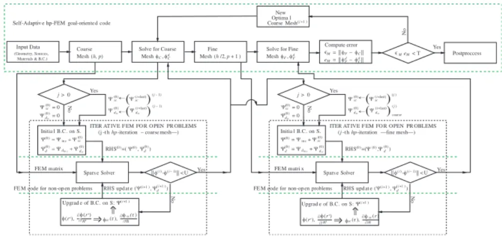
Figure 1. Flow chart of the self-adaptive hp methodology combined with the iterative FEM for open region problems (FE-IIEE).
2. SELF-ADAPTIVE HP-STRATEGY FOR OPEN REGION PROBLEMS
The automatic hp-adaptive algorithm for open region problems using a goal-oriented strategy is based on the energy-norm driven algorithm presented in [22]. Thus, the latter algorithm will be briefly reviewed here.
As it was mentioned, FE-IIEE is used as the mesh truncation methodology. The iterative nature of FE-IIEE and the automatic adaptivity itself yields a doubly nested loop algorithm (see Fig. 1). The dashed line box at the top includes the algorithm corresponding to the automatic hp-adaptivity. The relevant part of the flow chart of FE-IIEE is shown as module (dashed boxes at the bottom). As it will be clear later, the outer loop provides an optimal FEM hp-discretization for a given “continuous” problem cast in variational form. The FE-IIEE inner loop updates the right hand side of the discrete problem providing an arbitrarily accurate mesh truncation boundary condition. Provided that the error of the inner loop is low enough with respect to the error of the outer loop (U < T, see Fig. 1), the inner loop, although it works at the discrete level, may be seen as the one providing an exact boundary condition at the continuous level.
FEM hp-discretization supports 1-irregular meshes (i.e., with
hanging nodes) in terms of isoparametric quadrangles (also triangles)
of variable order of approximation supporting anisotropy. The self-adaptive strategy iterates along the following steps. First, a given
mesh, Then, the problem of interest is solved on the coarse and fine meshes. φC and φF are used to denote the field solution on the coarse and fine meshes, respectively. The difference between the fine and coarse grid solutions provides an error function (an error indicator is not enough) that is used to guide optimal refinements over the coarse grid (block “New Optimal Coarse Mesh” in Fig. 1). Details are quite involved and can be found in [26]. Roughly speaking, a “competition” betweenp-refinement with allcompetitive h-refinements takes place at each iteration step. The “competition” is driven by theerror decrease rate (EDR) of each edge of the mesh; being equal to
EDR =
°
°φh/2,p+1−Πhpφ°°−°°°φh/2,p+1−Πhpˆφ°°
°
(p1+p2−p) , (1) where Πφ stands for the projection based interpolation of φ. This operator is local, it maintains conformity and it is optimal in the sense that the error behaves asymptotically, both in h and p, in the same way as the actual interpolation error (see [26, 27] for details). Symbol ˆhp = (ˆh,pˆ) is such that ˆh ∈ {h, h/2}. If ˆh = h, then ˆ
p=p+ 1. If ˆh=h/2, i.e., the element is split, then ˆp= (p1, p2), where
p1+p2−p >0, max{p1, p2} ≤p+ 1. In other words, the competitive
h-refinements are those that result in the same increase in the number of d.o.f. as the p-refinement. Note that φh/2,p+1 corresponds to
φF of Fig. 1. Analogously, the winner of the “competition”, Πhpˆφ,
corresponds to theφC of the next coarse mesh.
The error (to be minimized), denoted ask·kin (1) is measured with the energy-norm of the problem that is obtained from an “energy” type inner product defined over H1 (defined later in (10)). In this paper,
2D scattering and radiation problems under TM and TE polarization are used to illustrate the presented approach. This problem may be modeled in scalar form and solved usingH1-conforming finite elements.
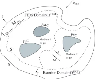
However, the adaptive strategy is very general, and it applies also to H(curl)- (see e.g., [20]), and H(div)-conforming discretizations. FE-IIEE is based on a two domain decomposition multiplicative Schwarz paradigm [28]. The original infinite domain is divided into two overlapping domains: a finite FEM domain (ΩFEM) bounded by surface
Sand the infinite domain exterior to the auxiliary boundaryS0(ΩEXT).
Thus, the overlapping region is limited by S0 and S (see Fig. 2).
The field in ΩFEMis modeled by Helmholtz equation,
∇t· £
fr−1∇tφ ¤
ε2µ2
Medium 2 ε1µ1
Medium 1
PEC
PEC PM C
S S’
ˆ
n
ˆn'
J
M
φinc
Meq
Jeq
FEM Domain(Ω FEM)
Exterior Domain( Ω EXT)
Figure 2. General scattering (or radiation) problem.
and suitable boundary conditions:
φ(ρ) = 0 ρ∈ΓD (3)
∂φ(ρ)
∂n = 0 ρ∈ΓN (4)
∂φ(ρ)
∂n +j β φ(ρ) = 2jβ φ
imp
Pi (ρ) ρ∈ΓPi (5)
∂φ(ρ)
∂n +j k0φ(ρ) = Ψ(ρ) ρ∈ΓS (6)
where the correspondences depending on the (TM or TE) polarization are given in Table 1: E, H denote electric and magnetic field, respectively, and εr, µr electric permittivity and magnetic
permeability, respectively, with respect to vacuum medium. Symbol
nstands for the outward normal to the corresponding boundary. The field denoted by φimpPi (which is not represented in the figure) is the impressed (incident) field at the i-th waveguide port of the structure; symbolβ denoting the propagation constant of the fundamental mode of the waveguide. Thus, q and φimpP
i are internal sources (radiation problem) while the incident field (a plane wave arriving from direction
ϕinc) constitutes the exterior excitation. The latter is introduced in
the mathematical model by plugging it into (6), i.e., ∂φinc(ρ)/∂n+
j k0φinc(ρ) = Ψinc(ρ). The function Ψ, and specifically, Ψinc will be
Table 1. Correspondences for scattering and radiation formulations. Pol. φ fr gr Io q ΓD ΓN
TM Ez µr εr ηo jk0I0Jz ΓPEC ΓPMC
TE Hz εr µr 1/ηo jk0I0Mz ΓPMC ΓPEC Pol. φ Lteq Oeqz
TM Ez Meqt =φ Jeqz = (∂φ/∂n0) /(jk0I0)
TE Hz Jeqt =φ Meqz = (∂φ/∂n0) /(jk0I0)
that a Cauchy boundary condition (see (6)) is used onS, thus, avoiding the interior resonance problem.
The variational formulation of the problem is obtained by multiplying (2) by a suitable test function ω, using the integration by parts, and finally including boundary conditions (4), (5), (6), in the integral formulation obtained. Thus, the formulation of the problem reads:
Find φ∈H1 such that
b(ω, φ) =f(ω) ∀ω ∈H01 (7) whereH1
0 :={p∈H1(Ω), p= 0 on ΓD}, sesquilinear form b,
b(ω, φ) =
Z
Ω
∇tω¯· £
fr−1∇tφ ¤
dΩ−k20gr Z
Ω
¯
ω φ dΩ +j k0fr−1
Z
ΓS
¯
ω φ dΓ +j βPi
Z
ΓPi
¯
ω φ dΓ (8)
and antilinear form f,
f(ω) =−
Z
Ω
¯
ω q dΩ +
Z
ΓS
¯
ωΨdΓ + 2j βPi
Z
ΓPi
¯
ω φimpPi dΓ (9) where the “bar” superscript denotes the complex conjugate.
From the above, an “energy”-type normk · k can be defined. The energy-norm of a given φiskφk=phφ, φi where the inner product is given by:
hω, φi =
Z
Ω
∇tω¯· £
fr−1∇tφ ¤
dΩ +k02gr Z
Ω
¯
ω φ dΩ +¯¯j k0fr−1
¯ ¯ Z
ΓS
¯
ω φ dΓ +|j βPi|
Z
ΓPi
¯
The field in ΩFEM can be obtained as the FEM solution of (7),
provided that the residual of the boundary condition on S (ΓS), i.e., Ψ, is known. The value of Ψ can not be known before solving the problem; however, it can be estimated from the exterior problem. The exterior domain ΩEXTis electromagnetically modeled with the Integral
Equation as the equivalent problem exterior toS0 using the equivalent
currents Jeq and Meq of ΩFEM (computed by means of the FEM
solution), and the Green’s function G of ΩEXT (a zero order second
class Hankel function for the free-space case). Thus, the scattered (or radiated field)φscthat has to be added to the field due to exterior sources (i.e., the incident fieldφinc) to yield the total fieldφis obtained
as:
φsc(ρ) = I
S0 ·
Lteq(ρ0)∂ G(ρ,ρ0)
∂n0 −jk0I0Ozeq(ρ0)G ¡
ρ,ρ0¢
¸
dl0 ρ∈ΓS
(11) where the superindexestandzrefer to the tangential and longitudinal components, respectively. The equivalent currents are defined in terms of φ, or its normal derivative, according to Table 1. The normal derivative of the scattered field is obtained by derivation of (11).
The total field φ calculated following this procedure, and its normal derivative, are plugged into (6) to get the new value for Ψ. Note that the solution of the interior problem is needed in order to get JeqandMeq. Thus, the whole problem is solved in an iterative fashion
resembling domain decomposition Schwarz iterations. An initial value Ψ must be chosen at the first iteration. A natural choice is Ψ(0) = Ψ
inc,
where Ψinc refers to the result of substituting φ by the incident field
φinc in (6). Thus, Ψ(0)= 0 for radiation problems.
Finally, the combination of FE-IIEE algorithm withhp-adaptivity algorithm implies that hp-discretized versions of (7), (11), and of the corresponding spaces, are used in practice.
3. GOAL-ORIENTED SELF-ADAPTIVE
HP-STRATEGIES FOR OPEN REGION PROBLEMS
The goal-orientedhp-adaptivity is built upon the algorithm presented in the previous section. Details about the algorithm itself are given in Section 3.1. Details about the implementation are given later in Section 3.2.
3.1. Theory
the error of the field in the whole domain (i.e., minimization of the energy-norm error). As it was mentioned in the Introduction, this is particularly relevant for open region problems.
It is assumed that the quantity of interest can be expressed as a continuous and linear functional of the field L(φ). If the quantity of interest is not continuous, a continuous approximationLto the original quantity of interest would be considered. Analogously, if the quantity of interest is represented by a non-linear functional, a linearization of it around a specific solution, and replacement of the original functionalL
with its linearized version, would be done. In this paper, the quantities of interest considered are:
• A transmission type scattering parameter, Sji(j6=i)
The parameter Sji, e.g., S21, between the ports of two antennas
(e.g., of an array antenna) reflects the mutual coupling level between those two antennas. Thus, for this case,
S21≡L(ω) = 2j βp2 Z
Γp2
ω φimpp2 dΓ (12) Note that the functional L defined above is identical to the last term on the right hand side of (9).
• The far field in a given direction ϕobs
The scattered or radiated field is given by (11). The far field approximation of it on a given direction ˆρ= exp(jϕobs) yields:
φ( ˆρ)≡L(ω) =
r
j k0
8π
I
ΓS0
µ ¡
ˆ
ρ0·ρˆ¢ω− 1
j k0 ∂ ω ∂n0
ej k0(ρ0·ρˆ)dΓ
(13) where coordinate ρ0 refers toS0 (Γ
S0).
Note that functional definition of (13) is easily extended to an interval, or range, of directions.
The functionals shown above are both continuous and linear functionals of φ. By recalling the linearity ofL, we have:
Error of interest =L(φ)−L(φhp) =L(e) (14) wheree=φ−φhp denotes the function of the error of the field.
Symbol φ stands for the solution of the problem and φhp for the approximation given byhp-FEM, i.e., by discretizing (7). Expressed in compact form, the discrete version of the variational formulation reads
as: (
Find φhp∈H01hp
b(ωhp, φhp) =f(ωhp) ∀ωhp∈H1
0hp
By defining the residual rhp(ω) = f(ω)−b(ω, φhp) = b(ω, φ−
φhp) =b(ω, e), we look for the solution of the dual problem:
(
Find ¯φd∈H1 0
b(φd, ω) =L(ω) ∀ω ∈H1 0
(16)
Solutionφdis usually referred to as theinfluence function. This is due to the fact that this function relates the error in φwith the error in the quantity of interestL(e).
The hp-discretized version of (16), shown below, is solved obtaining the discrete version of the solution of the dual problem,φd
hp: (
Find ¯φd
hp∈H01hp
b(φdhp, ωhp) =L(ωhp) ∀ωhp∈H01hp,
(17) Now, it is desirable to express the error in the quantity of interest in terms of the form b of the variational formulation of the problem. For that purpose, the definition of the dual problem is used. Thus, it can be written
L(e) =b
³
φd, e
´
=b
³
φd−φdhp
| {z } ²
, e
´
=b(², e) (18)
where Galerkin orthogonality between the error and the test (also basis) functions, b(ωhp, e) = 0, has been used.
At this point, it is worth explaining that, in practice, bilinear (and not sesquilinear) forms are used. This is possible due to the use of real valued test (and basis) functions. The bilinear form (denoted as ˜b) of the sesquilinear form b of (8) is obtained by simply deleting the complex conjugate from the expressions, i.e., writing ω instead of ¯ω. That means that the dual problem is solved for the complex conjugate of φd. However, as it will be clear later, it has no impact in the
goal-oriented adaptivity.
Once the error in the quantity of interest has been determined in terms of the bilinear form ˜b, a sharp upper bound for |L(e)| that depends upon the mesh parameters (element size h and order of approximationp) only locally, must be obtained. Then, a self-adaptive algorithm (similar to the one with the energy-norm described in the previous section) may be constructed.
As in the energy-norm based approach, a fine grid is used. The solutions, φ, φd, are approximated by the fine grid solutions, φh
2, p+1,
φd
h
2, p+1
Next, the error in the quantity of interest is bounded by a sum of element contributions. Let bK denote a contribution from element K
to sesquilinear form b. It then follows that |L(e)|=|b(², e)| ≤X
K
|bK(², e)| (19)
where summation overK indicates summation over elements.
Next, the upper bound of (19) is expressed in terms of local quantities, i.e., in terms of quantities that do not vary globally with local modifications of the grid. For this purpose, theprojection based interpolationΠhpφcomes into the picture as it does in the energy-norm
approach. A Galerkin projection operatorPhpis also defined such that
φhp=Phpφ. Thus, (19) becomes
|L(e)| ≤ X
K
|bK(², e)|
= X
K ¯ ¯
¯bK
³
², φ−Πhpφ
´
+bK ³
²,Πhpφ−Phpφ
´¯¯
¯ . (20)
Given an element K, the conjecture that |bK(²,Πhpφ−Phpφ)|
will be negligible compared to |bK(², φ−Πhpφ)| is made. Under this
assumption, it is concluded that: |L(e)| ≤CX
K ¯ ¯
¯bK
³
², φ−Πhpφ
´¯ ¯
¯. (21)
whereC is a positive constant (typically, close to one). In particular, for²=φd−Πhpφd, it is obtained:
|L(e)| ≤CX
K ¯ ¯
¯bK
³
φd−Πhpφd, φ−Πhpφ
´¯¯
¯. (22)
Finally, by applying Cauchy-Schwartz inequality, the next upper bound for|L(e)|is obtained:
|L(e)| ≤CX
K
k˜²kKk˜ekK, (23)
where ˜e = φ −Πhpφ, ˜² = φd − Πhpφd, i.e., the projection based
interpolation errors on φ and φd, respectively. Symbol k · k
K denotes
energy-normk · k (inferred by (10)) restricted to elementK.
the influence function φd. For instance, the error decrease rate EDR
defined on each edge, which is at the core of the self-adaptive hp -algorithm, is transformed from (1) for energy-norm approach into the following for goal-oriented approach (already expressed at the element level):
EDR = X
K
°
°φ
h/2,p+1−Πhpφ ° ° K
° °
°φdh/2,p+1−Πhpφd
° ° ° K
p1+p2−p
−
° °
°φh/2,p+1−Πhpˆφ°°°
K ° °
°φd
h/2,p+1−Π ˆ
hpφd°°° K
(p1+p2−p)
, (24)
3.2. Implementation Details
As it has been described above, the implementation of the goal-oriented
hp-adaptivity requires a few modifications on the energy-norm based
hp-adaptivity. First of all, in addition to the “original” problem, a second (dual) problem has to be solved on the same (coarse or fine) mesh. However, they both share the same bilinear form, i.e., they both have the same FEM matrix. Thus, the goal oriented approach requires the solution of the same algebraic system of equations with two different right hand sides. In particular, a multifrontal based direct solver (by interfacing with MUMPS library, [29]) is used to solve the system taking advantage of that fact. Also, norms used to measure the errors in the kernel of the self-adaptive procedure are doubled, in the sense that they have to include the contribution of the energy error of the dual problem. As a consequence, the computational overhead of the goal-oriented approach is minimum and the order of computational complexity is not altered with respect to the energy-norm approach.
It is worth noting here that the dual problem is also an open region problem and, hence, a mesh truncation scheme has to be provided. This is achieved again through FE-IIEE, i.e., by iterating in the inner loop of Fig. 1. In other words, the right hand side of the dual problem has to include the excitation term with the residual of the Cauchy type exterior boundary condition Ψ. Thus, dual problem (16) has to be reformulated as:
(
Find ¯φd∈H1 0
b(φd, ω) =L(ω) +R
ΓSω¯ΨdΓ ∀ω∈H
1 0
Another issue that is worthy of comment is the interaction between the outer and inner loops of Fig. 1. It can be seen in the figure that the inner loop of FE-IIEE takes action twice (solution of the problem on the coarse and the fine grids). Actually, in the goal oriented approach there are two different right hand sides, as it was mentioned above: one for the primal — original — problem and one for the dual problem. In total, the inner loop takes action four times per iteration of the
hp-adaptivity. However, the runs are not independent of each other, The information from previous iterations are used. First, at each step
j of the adaptivity the last residual Ψ of the previous step of the adaptivity is used to start the FE-IIEE iterations of the inner loop. Second, the discrete Ψ obtained in the last iteration of FE-IIEE of the coarse mesh is is used to start the FE-IIEE iterations for the fine mesh. In practice, two extra iterations of the iterative FEM for the fine mesh have demonstrated to be enough to guide the adaptivity. These interactions are depicted in Fig. 1.
In summary, the addition of the FE-IIEE inner loop to the original
hp-adaptivity for conventional closed domain problems is reduced to perform only a few iterations of the inner loop, so that the FE-IIEE iterations do not start from zero.
The computational cost of the FE-IIEE iterations is ofO(NSNS0)
whereNS,NS0 are the number of unknowns onS and S0, respectively.
Both NS and NS0 are proportional to NF EM1/2 (NF EM2/3 for 3D).
Therefore, the computational cost of the FE-IIEE iterations is of
O(NF EM) (O(NF EM4/3 ) for 3D) which is lower than the order of the
direct solution of the FEM system (either on coarse or fine meshes), which is of (O(Nα
F EM), where α is typically equal to 2; with intensive
presence of high p in the mesh, α can go slightly above 2. Thus, the inclusion of FE-IIEE iterations does not result on an increment of the computational complexity order.
What was mentioned before refers to the use of a non-accelerated convolution type product. In the code, a simple h-type adaptive integration technique has been implemented. However, as FE-IIEE iterations are decoupled from the FEM part and they involve a convolutional type product at each step, accelerated methods as FMM (Fast Multipole Method, [30]), ACA (Adaptive Cross
Approximation, [31]) and so on, are suitable to be applied. These
4. NUMERICAL RESULTS
Numerical results obtained from the application of the goal-oriented
hp-automatic adaptivity described above to several electromagnetic wave propagation problems in open domains are shown next. Specifically, results of mutual coupling between antennas, and results of the scattered far field produced by plane wave illumination of several objects, are considered. Goal-oriented results are compared with their analogous counterparts obtained by classical energy-norm driven adaptivity.
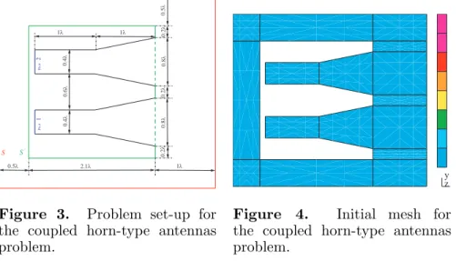
The first results correspond to the analysis of the mutual coupling between two horn-type antennas. Parallel plate waveguide technology is considered, thus allowing the 2D analysis of the problem. The problem set-up is shown in Fig. 3. It is important to note that the FEM domain can be reduced by placing S0 conformal to the metallic
parts and making the distanceS−S0 shorter. However, for illustration
purposes (better observation of the fields around the structure), it has been preferred to leave it as shown in Fig. 3. Mutual coupling is characterized by the scattering parameter S21 between the two
waveguide ports. TEM mode type excitation is considered.
For illustration purposes, a very coarse mesh (with first order finite elements) is chosen. The initial mesh is shown in Fig. 4. The scale on the right indicates the orderp of the elements (the dark blue being p = 1 and the pink p = 8); in this case, all is dark blue as it corresponds to uniform order p = 1. It is worth noting that, on a general hp-mesh (as those shown later), different colors inside an
Po rt 2 Po rt 1 S' S 0 . 2 λ 0 . 8 λ 0 . 8 λ 0 . 4 λ 0 . 2 λ 0 . 6 λ 0 . 5 λ
0.5λ 2.1λ 1λ
1λ 1λ 0 . 4 λ 0 .2 λ
Figure 3. Problem set-up for the coupled horn-type antennas problem.
y z
element represents anisotropic polynomial orders (different p in local vertical and horizontal directions) and/or different orders for edges or interior. The initial mesh and the geometry are defined in aninput file, using the graphical user interface with a general pre and post-processor described in [32].
From that initial mesh, and following the automatic iterative procedure described above, hp-meshes are obtained by refining simultaneously in h and p the hp mesh of the previous step. In this case, as explained in Section 3, the functionalLthat corresponds to the excitation of the dual problem, is given by (12). Thus, the influence function φd corresponding to the field solution of the dual problem is simply obtained by solving the original two-antenna problem but exciting port 2 instead of port 1.
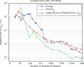
The comparison in the evolution of the error in the quantity of interest, i.e., S21, between the conventional energy-norm adaptivity and the goal-oriented approach presented in this paper is shown in Fig. 5. It is observed how goal-oriented adaptivity achieves a given error in a much lower number of iterations of the adaptivity (and with a much lower number of unknowns) than the energy-norm driven adaptivity. For instance, for an error in S21 lower or equal to 1%,
21 iterations are needed when using the energy-norm adaptivity in contrast with only 7 iterations when using the goal-oriented approach.
8 64 216 512 1000 1728 2744 4096
10-1 100 101 102 103
Number of degrees of freedom
Relative error of |S
21
| (%)
Coupled horns with TEM Mode
Energy Goal S21
Upper Bound of Relative Error: S21
Correspondingly, the number of unknowns is 1905 in contrast with 384. Equivalently, for a given number of unknowns, the error with goal-oriented is smaller than the one with energy-norm. In this case, the difference in the error levels is approximately one order of magnitude. The upper bound of (23) is also shown in Fig. 5. It can be observed, as predicted by the theory, an exponential rate of convergence of the error for the bound, after the initial pre-asymptotic regime. By exponential convergence it is meant that error =
Cexp(−Nα
dof) in the asymptotic regime, where Ndof is the number
of unknowns. Specifically, the theory according to [33] predicts that
α= 1/3 for 2D. Thus, the exponential convergence behavior is shown as a straight line when plotting the error in logarithmic scale versus
Ndof1/3. This is precisely how the scales of the plots shown in the paper have been set up. Note that the abscissa scale corresponds to Ndof1/3
while abscissa axis tics should be read as Ndof in the plots.
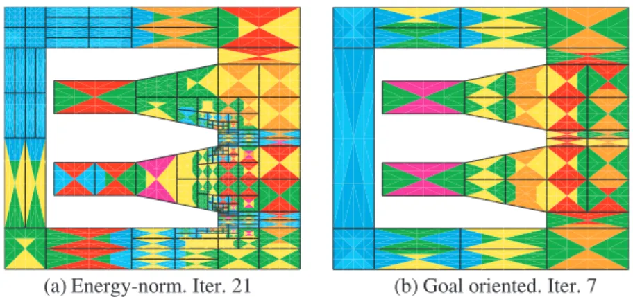
The explanation for the behavior of the error with the number of unknowns shown in Fig. 5 is clear when looking at the hp-meshes delivered by both types of adaptivity. Fig. 6 shows an example of each type corresponding to approximately the same error in S21.
The hp-mesh corresponding to energy-norm adaptivity, Fig. 6(a), shows a higher number of refinements, specially in h, due to the need of capturing the diffraction type of phenomena that produces the coupling between both antennas. In contrast, the hp-mesh corresponding to goal-oriented adaptivity, Fig. 6(b), reflects a low number of refinements, specially in p, as it would correspond to the interpolation of a smooth solution. This is because the goal-oriented adaptivity is driven by the error estimation due to the field solution
(a) Energy-norm. Iter. 21 (b) Goal oriented. Iter. 7
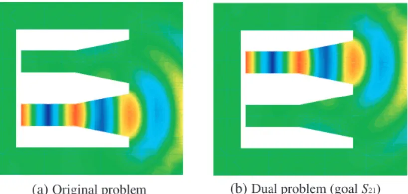
(a)Original problem (b)Dual problem (goal S21)
Figure 7. Real part of the field for the coupled horn-type antennas (original and dual) problems.
of both, the original — primal — and the dual, problems. The field solution of the dual problem is shown in Fig. 7. It can be observed that, as it was mentioned above, the dual problem is simply the original problem but with the excitation on the “other” port. Note that, due to the symmetry of the initial mesh, hp-meshes delivered by the goal-oriented adaptivity are also symmetric.
It is important to note that there are no special refinements (in the form of boundary layers or similar) close to the truncation boundary, as it happens with other mesh truncation techniques, for instance, with PML. The same comment can be made about the rest of thehp-meshes shown in this paper.
From the results mentioned above, it may be concluded that goal-oriented adaptivity outperforms energy-norm adaptivity for the characterization of mutual coupling between antennas. This conclusion, together with those obtained in [20] relative to closed domain (waveguide discontinuity) problems, somehow completes the research on the viability and performance of goal-oriented adaptivity for computation of scattering parameters. The main conclusion is that goal-oriented adaptivity is clearly more efficient than energy-norm adaptivity for the computation of “transmission” parameters relating two ports loosely coupled. The low coupling can happen because of dissipative losses, as it was the case of one example of [20], or because of the “free space losses” as it is the case of the radiation example above.
the incident wave are considered. Thus, a 2D analysis of the problem is possible. Perfect electric conducting (PEC) objects have been considered. Several shapes have been analyzed (circular, square, etc). For the sake of brevity, only results of the circular shape PEC cylinder are shown. Radius of the circular cylinder is a=λ. Mesh truncation boundary S and auxiliary boundary S0 are also circular, placed 0.2λ
and 0.1λ away, respectively. The initial mesh used in the analysis is shown in Fig. 8. Incidence direction ϕinc = 0◦ is considered. TM and
TE polarizations were considered. There were not found any significant differences between both polarizations results. Then, for the sake of brevity, only results corresponding to TM polarization are shown next. The quantity of interest in this case is the far field in a given direction. Thus, the functional L that corresponds to the excitation of the dual problem, is given by (13). Thus, the influence function corresponding to the field solution of the dual problem does not have a clear physical meaning, as in the case of choosing the scattering parameters Sji as quantities of interest.
The first case considered is the far field in ϕobs = 90◦ resembling
a bistatic RCS (Radar Cross Section) computation. Fig. 9 shows the comparison in the evolution of the error in the quantity of interest between the classical energy-norm adaptivity and the goal-oriented approach presented in this paper. It is observed how goal-oriented adaptivity outperforms energy-norm driven adaptivity. As illustration,
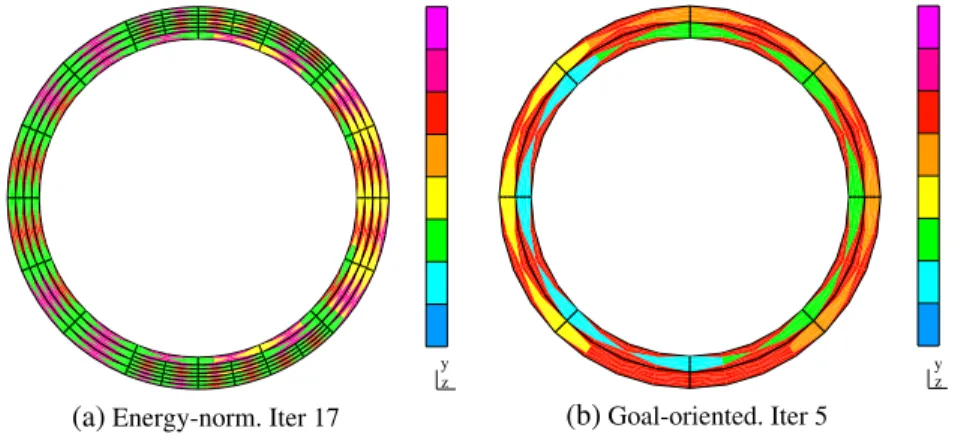
hp-meshes delivered by the automatic adaptivity with both approaches for an error around 0.001% are shown in Fig. 10. Only 6 iterations are needed with goal-oriented in contrast to 18 iterations with energy-norm adaptivity. Analogous statements as those made with the radiation problem with respect the hp-meshes are valid here. In this case, intensive h-refinements with the energy-norm approach occur around
y z
the transition between the illuminated and lit regions (diffraction like points).
Results of the circular shape scatter with the far field in ϕobs =
0◦ as the quantity of interest, i.e., resembling a monostatic RCS
computation, are shown next. The behavior of the error is similar to the one of ϕobs = 90◦ (Fig. 9) and is omitted. The hp-mesh delivered
8 64 216 512 1000 1728 2744 4096 5832 8000 10-6
10-5 10-4 10-3 10-2 10-1 100 101 102
Number of degrees of freedom
Relative Error of quantity of interest (%)
Scattering Far Field φ=90 . PEC circular cylinder. φinc=0 hp Energ hp Goal
o o
Figure 9. Convergence history. Comparison of energy-norm adaptivity and goal-oriented approach with the far field in ϕobs = 90◦
as the quantity of interest for circular shape scatter.
y z
y z
(a) Energy-norm. Iter 17 (b) Goal-oriented. Iter 5
Figure 10. Meshes corresponding to relative error of ε ' 0.001% in the quantity of interest (quantity of interest is the far field at
y z
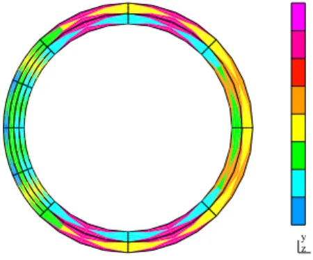
Figure 11. Mesh corresponding to 5-th iteration of goal-oriented automatic adaptivity (quantity of interest is the far field atϕobs = 0◦)
for circular shape scatter.
by the 5-th step of the goal-oriented strategy for this case is shown in Fig. 11. If that mesh is compared with Fig. 10(b), it is observed that the meshes are quite different. In other words, the implemented goal-oriented adaptivity presented in the paper distinguishes the different goals and guides the automatic adaptivity accordingly.
5. CONCLUSIONS
A fully automatic goal-oriented hp-adaptivity for scattering and radiation problems has been presented. The methodology has shown to produce exponential rates of convergence in terms of an upper bound of an user-prescribed quantity of interest. The computational overhead caused by the introduction of a goal-oriented strategy, with respect to the energy-norm driven adaptivity, is minimum, and the order of computational complexity is not altered. Its application to several scenarios has shown that goal-oriented adaptivity performs equally or better than energy-norm adaptivity in all cases, clearly outperforming it in most of the cases of interest. Thus, it may be concluded that it is worth using goal-oriented adaptivity. Finally, this work completes the research on the viability and performance of goal-oriented hp-adaptivity initiated in the context of computation of scattering parameters for waveguiding problems.
ACKNOWLEDGMENT
REFERENCES
1. Rheinboldt, W. C. and I. Babuˇska, “Error estimates for adaptive finite element computations,” SIAM Journal of Numerical Analysis, Vol. 15, 736–754, 1978.
2. Jin, J. M., The Finite Element Method in Electromagnetics, 2nd Edition, John Wiley & Sons, Inc., 2002.
3. Salazar-Palma, M., T. K. Sarkar, L. E. Garc´ıa-Castillo, T. Roy, and A. R. Djordjevic, Iterative and Self-adaptive Finite-elements
in Electromagnetic Modeling, Artech House Publishers, Inc.,
Norwood, MA, 1998.
4. Ping, X. W. and T. J. Cui, “The factorized sparse approximate inverse preconditioned conjugate gradient algorithm for finite el-ement analysis of scattering problems,” Progress In Electromag-netics Research, Vol. 98, 15–31, 2009.
5. Tian, J., Z. Q. Lv, X. W. Shi, L. Xu, and F. Wei, “An efficient approach for multifrontal algorithm to solve non-positive-definite finite element equations in electromagnetic problems,”Progress In
Electromagnetics Research, Vol. 95, 121–133, 2009.
6. Borouchaki, H., T. Grosges, and D. Barchiesi, “Improved 3D adaptive remeshing scheme applied in high electromagnetic field gradient computation,” Finite Elements in Analysis and Design, Vol. 46, 84–95, 2010.
7. Mitchell, W. F. and M. A. McClain, “A comparison of hp-adaptive strategies for elliptical partial differential equations,” Tech. Rep.
NISTIR-7824, National Institute of Standards and Technology
(NIST), 2011.
8. Botha, M. M. and D. B. Davidson, “P-adaptive FE-BI analysis of homogeneous, lossy regions for SAR- and far-field calculations,” IEEE Antennas and Propagation Society
International Symposium Digest, 684–687, Institute of Electrical
and Electronics Engineer, Columbus, Ohio, USA, 2003.
9. Nair, D. and J. P. Webb, “P-adaptive computation of the scattering parameters of 3-D microwave devices,” IEEE
Transactions on Magnetics, Vol. 40, No. 2, 1428–1431, 2004.
10. Ren, Z. and N. Ida, “Solving 3D eddy current problems using second order nodal and edge elements,” IEEE Transactions on
Magnetics, Vol. 36, No. 4, 746–749, 2000.
11. Andersen, L. S. and J. L. Volakis, ‘Adaptive multiresolution antenna modeling using hierarchical mixed-order tangential vector finite elements,” IEEE Transactions on Antennas and
12. Sheng, Y., R. Chen, and X. Ping, “An efficient p-version multigrid solver for fast hierarchical vector finite element analysis,” Finite
Elements in Analysis and Design, Vol. 44, 732–727, 2008.
13. Ledger, P. D., K. Morgan, J. Peraire, O. Hassan, and N. P. Weatherill, “The development of an hp-adaptive finite element procedure for electromagnetic scattering problems,”
Finite Elements in Analysis and Design, Vol. 39, 751–764, 2003.
14. Ingelstr´om, P., V. Hill, and R. Dyczij-Edlinger, “Goal-oriented error estimates for hp-adaptive solutions of the time-harmonic Maxwell’s equations,”IEEE/ACES Int. Conf. Wireless
Communications and Applied Computational Electromagnetics,
396, 2006.
15. Rachowicz, W. and A. Zdunek, “An hp-adaptive finite element method for scattering problems in computational electromagnet-ics,”International Journal for Numerical Methods in Engineering, Vol. 62, No. 9, 1226–1249, 2004.
16. Zdunek, A., W. Rachowicz, and N. Sehlstedt, “Toward hp-adaptive solution of 3D electromagnetic scattering from cavities,”
Computer and Mathematics with Applications, Vol. 49, 23–38,
2005.
17. Oden, J. and S. Prudhomme, “Goal-oriented error estimation and adaptivity for the finite element method,” Computer and
Mathematics with Applications, Vol. 41, No. 5–6, 735–756, 2001.
18. Sun, D. K., Z. Csendes, and J.-F. Lee, “Adaptive mesh refinement, h-version, for solving multiport microwave devices in three dimensions,” IEEE Transactions on Magnetics, Vol. 36, No. 4, 1596–1599, 2000.
19. Ingelstr´om, P. and A. Bondeson, “Goal-oriented error-estimation for S-parameter computations,” IEEE Transactions on Magnet-ics, Vol. 40, No. 2, 1432–1435, 2004.
20. Garc´ıa-Castillo, L. E., D. Pardo, and L. F. Demkowicz, “Energynorm based and goal-oriented automatic hp adaptivity for electromagnetics: Application to the analysis of H-plane and E -plane rectangular waveguide discontinuities,”IEEE Transactions
on Microwave Theory and Techniques, Vol. 56, No. 12, Part 2,
3039–3049, 2008, doi:10.1109/TMTT.2008.2007096.
21. Nguyen, D. T., J. Qin, M. I. Sancer, and R. McClary, “Finite element-boundary integral methods in electromagnetics,” Finite
Elements in Analysis and Design, Vol. 38, No. 5, 391–400, 2002.
electromagnetics,” IEEE Transactions on Magnetics, Vol. 43, No. 4, 1337–1340, 2007.
23. Zdunek, A. and W. Rachowicz, “A goal-oriented hp-adaptive finite element approach to radar scattering problems,”Computer
Methods in Applied Mechanics and Engineering, Vol. 194, No. 2–5,
657–674, 2005.
24. Gomez-Revuelto, I., L. E. Garcia-Castillo, D. Pardo, and J. Kurtz, “Automatic hp adaptivity for three dimensional closed domain electrodynamic problems,”10th International Workshop on Finite
Elements for Microwave Engineering, New England, USA, 2010.
25. Gomez-Revuelto, I., L. E. Garcia-Castillo, D. Pardo, J. Kurtz, and M. Salazar-Palma, “Automatic hp-adaptivity for three dimensional electromagnetic problems. application to waveguide problems,” Higher Order Finite Element and Isogeometric
Methods, Cracow, Poland, 2011.
26. Demkowicz, L.,Computing with Hp Finite Elements. I. One- and
Two-Dimensional Elliptic and Maxwell Problems, Chapman &
Hall/CRC Press, Taylor and Francis, 2007.
27. Demkowicz, L. F. and A. Buffa, “H1, H(curl) and H
(div)-conforming projection-based interpolation in three dimensions. Quasi optimal p-interpolation estimates,” Computer Methods in
Applied Mechanics and Engineering, Vol. 195, No. 24, 4816–4842,
see also ICES Report 04-22, 2006.
28. Quarteroni, A. and A. Valli, Domain Decomposition Methods for Partial Differential Equations, Oxford Science Publications, 1999. 29. MUMPS Solver, http://www.enseeiht.fr/lima/apo/MUMPS/. 30. Coifman, R., V. Rokhlin, and S. Wandzura, “The fast multipole
method for the wave equation: A pedestrian prescription,”IEEE
Antennas and Propagation Magazine, Vol. 35, No. 3, 7–12, 1993.
31. Bebendorf, M., “Approximation of boundary element matrices,”
Numerische Mathematik, Vol. 86, No. 4, 565–589, 2000.
32. Garcia-Do˜noro, D., L. E. Garc´ıa-Castillo, and I. G´omez-Revuelto, “An interface between an hp-adaptive finite element package and the pre- and post-processor GiD,” Finite Elements
in Analysis and Design, Vol. 46, No. 4, 328–338, 2010,
doi:10.1016/j.finel.2009.11.005.
33. Babuˇska, I. and B. Guo, “Approximation properties of the hp-version of the finite element method,” Computer Methods in