Multiple solutions and numerical analysis to the dynamic and stationary models coupling a delayed energy balance model involving latent heat and discontinuous albedo with a deep ocean

Multiple solutions and

numerical analysis to the

dynamic and stationary

models coupling a delayed

energy balance model

involving latent heat and

discontinuous albedo with a

deep ocean

J.

1.

Díaz

1,

A. Hidalg0

2

and L. Tell0

3

1 Instituto de Matemática Interdisciplinar and Dept. Mat. Aplicada, Universidad Complutense de Madrid, E-28ü4ü Madrid, Spain. e-mail:

[email protected]

2 Dept. Matemática Aplicada

y

Métodos Informáticos. E.T.S.1. Minas

y

Energía, Universidad Politécnica de Madrid, E-28üü3 Madrid, Spain. e-mail:

[email protected]

3 Dept. Matemática Aplicada, E.T.S. Arquitectura, Universidad Politécnica de Madrid, E-28ü4ü Madrid, Spain. e-mail:

[email protected]

1. Introduction

This paper presents new contributions on the mathematical study of aclimate model coupling atmosphere and ocean under a simplified formulation. Our main goal is to exhibit the possible multiplicity of solutions due to presence of an abruptly distributed coalbedo, such as it was formulated in terms of a discontinuous function by the climatologist M.L Budyko (see [13]). Among the new effects considered with respect to previous mathematical treatments in the literature we consider here a positive latent heat for the ocean and a general memory term for the top ocean surface temperature. Moreover, we present here the numerical approximation of solutions by means of finite volume methods. We shall indicate also many other references on the mathematical treatment of this class of problems, in a survey style, trying to be useful in the necessary dialog between geophysical and mathematician experts.

Our model tries to understand the deterministic interactions between two of the main components of the climatic system.Itis well known that detailed mathematical models of the atmosphere, the ocean and ice sheets are available (see, for instance, the proceedings of several meetings devoted to this topic, as it was the case of the references [33], [27], [28] and [12]). Nevertheless, investigating inherently transient phenomena with periods of 100 to 100,000 years is, of course, out of question for such sophisticated models. This is one reason why simpler models form useful tools in theoretical climatology. In addition, the mathematical treatment of such models is far to be obvious and requires the application of finer techniques of the mathematical and numerical analysis of nonlinear partial differential equations.

Our model takes in account, at least implicitly, the multiple spatial scales which arise in such complex coupling. Indeed, instead of considering the atmosphere temperature we shall work, as usual in the theory of EBM, with the averaged surface temperature on suitable spacial and time local scales.Itis well known that in spite of its simplicity, this kind of averaged equations preserve a high sensitivity with respect to solar parameters. This is very useful for the study in very large time scales. Nevertheless, since the heat capacity of the ocean is so large, any departure from equilibrium in the ocean must have a fairly large effect on the thermodynamic state of the atmosphere. As for the ocean, although we can also simplify its modelling we must maintain the fact that cold water in a few localized regions at high latitudes sinks is distributed throughout the deep ocean by currents and slowly rises towards the surface. So, following [70], we maintain the ocean depth scale for the deep ocean and identify the ocean mixed layer with the averaged atmospheric surface. This type of models allows to find sorne explanations to the Glacial-Holocene transition (see [70]). The inclusion of sorne stochastic internal and external variations imperfectly known, as it is the case of solar luminosity variations, volcanic aerosols andC02,have already studied for the associate surface EBM (see, e.g. [56], [45], [23], [36]).

past glaciations where obtained in [54]. Here we shall only include a delayed term in the deep ocean temperature equation following the approach initiated in the papers [14], [63], [21], [46], etc., to simulate seasonally-varying internal parameters.

As said before, even if the model under consideration responds to simplified modelling arguments, the presence of several nonlinear terms, sorne of them not always differentiable, makes that its mathematical treatment can not be reduced to the mere direct application of the differential delayed equations (DDE) theory (see, e.g. [47] and [71]). In Section 2 we state the model under consideration and the main structural and constitutive assumptions. The study of solutions of the transient regime is presented in Section 3. Since there is no hope to get classical solutions of the system, we introduce the notion of weak solution we shall deal with. We prove the existence of such type of solutions under quite general assumptions on the data and, which is more unusual in the study of parabolic type systems, we prove that, in general, there is no uniqueness of solutions when the coalbedo is assumed to be discontinuous. Since we also prove that, in this case, there is a continuum of solutions for suitable initial data, it is not possible to apply the results of the classical bifurcation theory for transient systems. Instead of that, we prove the uniqueness of weak non-degenerate solutions (corresponding to the case in which the atmospheric surface temperature arrives not too flat near the boundary of the region where the coalbedo changes, Le. on the surface where it becomes abruptly discontinuous). Let us recall that new aspects which have been taken into consideration in this type of coupled models are the ocean latent heat and the presence of a memory termo

Once we know the global existence of solutions on any arbitrary time horizonT it can be proved (see [30] and [64] for a special case of the present system) that the assumptions made here on the data exclude any other elements in the omega limit set (whent---++(0) different than the solutions of the stationary system. Perhaps this is the moment to point out that in many other systems the memory may lead to different qualitative properties of solutions with respect to the same system but without memory. We shall not develop this approach here but we refer the reader to a series of papers where this philosophy was carried out for different types of delayed systems (see [15], [16] and [17].

Coming back to the consideration of the associated stationary system, we show, in Section 4, the multiplicity of solutions in terms of the solar constantQ.Again, our result is not an automatic application of the general bifurcation theory but requires the construction of suitable families of super and subsolutions well adapted to our setting. An S-shaped bifurcation curve can be obtained in sorne special cases (see [2]).

The aboye mentioned mathematical analysis of the model allows to start the study of the controllability of sorne models connected with the climate system and, in particular with EBMs and related problems (see [25] and [26] for the case of a single EBM equation and [34] and [20] for sorne related problems). Moreover, it is possible to get a mathematical meaning to the proposals already present in sorne late works by J. von Neumann (see [68] and [29]).

Finally, in Section 5, we present several numerical experiments on the coupled model by means of a finite volume approach with WENO-7 spatial reconstruction and third order TVD Runge-Kutta for time discretization (for the application of the finite element method see [9]). We compare the numerical solution of the model with and without the effect of the ocean latent heat, and we also present a numerical experiment carried out by considering the effects of the memory termo Although the data in such experiments could be made more realistic we think that the main value of such numerical approach is to show how it is possible to made accessible to the quantification sorne sophisticated mathematical analysis of complex nonlinear systems, involving, for instance discontinuous albedo data, for which the solutions satisfy the requirements only in a weak sense. As Jacques-Louis Lions (1928 - 2001) said:

if

we accept that a model without data is a worthless

2. The mathematical model

Energy Balance Models (EBMs) were introduced, independently by M.1. Budyko [1969] andW.D. Sellers [1969] (sorne pioneering model is due to S. Arrhenius in 1896). Such type of climatological models have a diagnostic character and intended to understand the evolution of the global climate on a long time scale (see, e.g. [19],[48], [45]).Their main characteristic is the high sensitivity to the variation of solar and terrestrial parameters. They have been used in the study of theMilankovitch

theoryof the ice-ages (see, e.g.[54]).

The EBMs study a distribution of surface atmospheric temperature,u(t, x),which is expressed pointwise after sorne averaging process in space (the spatial variable x is in a small neighborhood

Bó(x) in the Earth's surface) and in time (on a small interval(t -

t,

t

+

t))

1

ft+t

f

u(t,x)

=

T(a,s)dads.

2tIBó(x)1

t-t

Bo(x)

The pointwise temperature T(a, s) is obtained from the thermodynamics equation of the

atmosphere primitive equations(see e.g.,[53]for a mathematical study of those equations and[52],

[31] for the application of averaging processes in this context).

More simply, the energy balance model can be formulated by using the energy balance on the Earth's surface: internal energy flux variation= R a - Re

+

D, where R a (respectively Re) represents the absorbed solar (resp. the emitted terrestrial energy flux) and whereD is the surface heat diffusion. By identifying the Earth's surface with a compact Riemannian manifold without boundaryM (for instance, the sphere 52 inlR3_{),the distribution of temperature,u(t,x),becomes}

a function of the spatial x andttime variables. The time scale is considered relatively long. The

absorbed energy Ra depends on the planetary coalbedo (3. The coalbedo function represents the

fraction of the incoming radiation flux which is absorbed by the surface. In ice-covered zones, reflection is greater than over oceans, therefore, the coalbedo is smaller. One observes that there is a sharp transition between zones of high and low coalbedo. In the energy balance climate models, a main change of the coalbedo occurs in a neighborhood of a critical temperature for which ice become white, usually taken as u = -100

e.

The coalbedo can be modelled by different monotone increasing fuctions (discontinous in case ofBudyko model and Lipschitz continuous

forSellers model).A more realistic albedo parametrization can be obtained by assuming that the

coalbedo fuction(3also depends on the spatial coordinates of each point of the Earth (specially on its latitude: see[48],Section3.3).Here we mainly consider the Budyko model since it produces more clear answers when one studies the evolution of the ice caps.

With respect to the surface temperature diffusion we send the reader to the modeling performed for instance in [45] for the case of a linear second order differential operator. Nevertheless, a quasilinear diffusion operator of the type div(k(x, u, Vu)Vu) was proposed in Stone [1971] as a better eddy diffusive approximation to account for the effect of large scale atmospheric circulation, wherek(x, u, Vu)is a non linear eddy diffusion coefficient, in particular,

k=b(x)

IVul.

In our model, we shall follow Stone's approach to represent the eddy diffusive

terms by settingk(x,u, Vu) =k(x)

IVul

p- 2,withp2:2andk(x)

>

a> O.

With respect to the simplified model on the deep ocean we shall follows the modeling derived in [70] but adding a positive latent heat, " which plays an important role in the formation of ice sheets. With respect to the memory term we recall that such type of terms were proposed for the study of ENSO events. For instance, in [63] it is takenQ(t, x, u, u(t - T)) = -u

+

u3

+

au(t - T),

for sorne a,T

>

O.We could include also sorne memory terms inside the albedo and latent heat expressions (as in[58])but the detailed mathematical treatment is much more technical. Notice that since u will be a globally bounded function, without lost of generality, we can modify the previous example function outside a compact of IF!(2 (concerning the values ofu and u(t - T)) in order to get a globally Lipschitz function. Obviously, the case Q(t, x, u, u(t - T))=Q(t, x, u)

s

<

0,

s=O,

s>

0,

Summarizing, our model will represent the interior and surface temperature of a global ocean

D,so that, the unknown are respectively given byU:D x [0,T]---+IRand byu:M x [-T,T]---+

IR,for an arbitraryT

>

O. Here we assume

(HI) Dis a bounded and open set ofIR3with maximum depthH andoD

=

M UN. M and

N

are COO

two dimensional compact connected oriented Riemannian Manifold ofIR3

without boundary and dist(M, N)

=

H.

Let(P3D)be the problem

O,(U) _ div(VU)

+

woU 3

°

in(O,T) x D,

8t

oz

o u . p-2 oU

8t - d¡v(IVMul VMU)

+

on

+

F(x,VMU)

+

Q(t, x, u, u(t - T))E

1

E-QS(t, x)(3(u)

+

f(t, x) in(O,T) x M, pe

UI[O,T]XM=u,

, OU

F(x,VNU)

+ a;;

=

°

in (O,T) x

N,

U(O, x, z)

=

Uo(x, z) inD,

u(s,·)

=

uo(s,') on[-T,O] x M.

Here VM and div are understood in the sense of the Riemannian metric on M (see, e.g. [38] and [53]). The rest of structural conditions are the following:

(H2) (3is a bounded maximal monotone graph, Le. Ivl :::;Mfor allvE(3(s),and allsED((3)

=

IR.

(H3) , is the graph

withk1

>

0, k2

>

°

andL

>

O.

(H4) Q: (O,T) x MxIF!( x IF!(---+IF!(is a continuous function, Q(t,x,eY,r¡) is a globally Lipschitz function with respect to eY (Le. u) and r¡ (Le. u(t - T)), such that Q(t, x,0, O)

=

°

and IQ(t,x, eY,r¡)I2: C(leYlr

+

I77n

for sorner

>

O.MoreoverT 2:O.

(H5) S:(O,T) x M ---+IR, Sl 2:S(t, x)2:So

>

°

a.e.xEM.

(H6) fE LOO ((O,T) x D).

(H7) F: M x T M ---+ IRand

P :

N

x T

N

---+ IRare linear on the tangent bundle spacesT M

andT

N

with bounded coefficients. (H8) W EC1

(n}

Remark 2.1. We point out that, for simplicity, we have assumed here isotropic (and constant) diffusion matrices in both equations. The mathematical treatment of the case of non constant definite positive diffusion matrices is quite similar and we drop the details.

Remark 2.2. The case in which the Solar constantQisassumed, in fact, as a periodic or almost periodic time function has been intensively studied in the literature (see, e.g. [45], [4] and its many references).

defined on[0, T] x [-1,1]:Le, hereM ={(x,O): x E [-1, 1]}:= ro)coupled with a 2d deep ocean (f?= [-1,1] x [0, -H],and so of boundaries

N

={(x, -H): xE [-1, 1]}:= rH,r-1:= {( -1,z) : ZE[-H,O]}andr1:={(1, z) : z E[-H,OJ}).The resulting equations ofthe model (this time with nonisotropic diffusion coefficients and with F(x,VMU) :=wXUxand F(x,VNU) :=wxUxand with a parameterD

>

°

modeling the mixed layer depth) now with x

=

sin'P, 'Prepresenting the latitude, andZE [-H,O],are the following:

,(U)t -

(~~

(1 - x2)Ux

h -

KvUzz

+

wUz 3

°

in f? x (O,T),

wxUx

+

KvUz

=

°

inrH x (O, T),

DKH ( 2 /2 - 2 )

au

DUt-~ (l-x)P luxl P _{Ux x +Kvan +wxUx+Q(t,x,u,u(t-T))E}

E

~S(t,

x)Q{3(u)

+

f(t, x) inro x (O,T), pe

UI[O,T]X[-l,l] =u,

(1-x2)Ux=0 in(r-1 x (0,T))U(r1 x (O,T)),

U(O, x,z)

=

Uo(x,z) in f?,

u(s,x,O) =uo(s,x,O) on[-T,O] x ro· (P2D)

Remark 2.3. We note that we can introduce the change ofvariable U

=

a(V),witha:=,-1,and then the equation in the inner ocean can be written as

where

{ S

kl a(s)

=

°

¿(s-L)

if

s

<

0,

if

0<

s

<

L,

if

s>

L.

(2.1)

The terms , anda(as well as {3) are maximal monotone graphs (see [11]). The main difference between ,

and a isthat , is always multivalued (once we assume L> O) although, in the atmosphere tempera ture

equation, the coalbedo {3 becomes a multivalued graph only when it is associated to a discontinuous coalbedo function, such as it was proposed in [13]. This is the reason why in the previous inner ocean equation and

the surface EBM it appears the symbolsEand3instead of the usual equality symbol.

3. On the evolution problem

3.1Existence of solutions.

WedefinethefunctionalspaceV:= {uE L2(M) :VMUELP(TM)}, whereTM

=

UpEMTpM

is the tangent bundle space (see [3]). Due to the presence of possible multivalued graphs (associated to discontinuous functions), and the possible choicep

el

2, we can not expect to solve the system in a classical sense but only in a weak way.

We say that the pair (U,u) with UEC([O,T] :L2(f?)), uEC([-T,T] :L2(M)) is a bounded weak solution of(P3D )if

(i) (U, u)ELCXJ((O, T) x f?) x LCXJ (( -T, T) x M)

n

L2(0, T: H1(f?)) x LP(-T, T: V),

(ii) there exist ZELCXJ((O, T) x f?) and hE LCXJ (( -T, T) xM) with ZE,(U) a.e. (t, x)E

t

Z(T,x)4>(T,x)dA- J:(4)t(t,x),Z(t'X))Hl(D)XHl(D)'dt+

J:

t

VUV4>dAdH

fT f oU fT f oU fT f

+

o Dwa;;4>dAdt - o M on 4>dS dt

+

O N F(x,VN)4>dS dt

=

t

Uo(x)4>(O,x)dA,

and

fM u(T,x)1jJ(T,x)dA- J:(1jJt(t,X),U(t,X))V'

xv

dt+

J:

fM IVulp- 2VuV1jJdSdH

+

J:

fM Q(t,x,u,u(t - T))1jJdS dt

+

J:

fM

~~

1jJdS dt

+

J:

fM F(x,VM)1jJdS dt

=

J:

fM QS(t,x)h(t,x)1jJdAdt

+

J:

fM f1jJdAdt

+

fM uo(O,x)1jJ(O,x)dS

for every test function (4), 1jJ)EL2(O,T:H1(f?)) x LP(-T, T) :W1,p(M)) such that (4)t, 1jJt)E

L2(0,T;H1(f?n x LP'(O, T; Vi). Here

<,

>v'xv

denotes the duality product inVi x V.

Theorem 3.1. Let UoELCXJ(f?) and UoEC((-T,O]: LCXJ(M)). Then there exists at least a bounded weak global solution of (P3D ).

Proa! We write the inner ocean equation as

oV _ div(Va(V))

+

w oa(V)

=

°

in (O,T) x f?,

8t

oz

with U

=

a(V) and a:=,-1, as mentioned in the aboye Remark 2.3 (notice that now a is singlevalued and so we do not need the symbol E). We approximate the maximal monotone graph a by some smooth increasing functions aE'Then we obtain a family of new problems, that we shall denote by(PE)'The main idea to solve(PE)is to apply Theorem 5.3.1 of [69] related to abstract functional equations. We shall construct an operator

Te

and to find a fixed point of it leading to a solution of(PE)'This will consist of several intermediate steps.

Step1. For everyhELCXJ((O, T) x M)we consider the problem(Ph,E)by replacing the coalbedo term in(PE) by h. The proof of the existence of solution of (Ph,E) is inspired in [35] and [7]. We define the vectorial operator AEbyAE(U, u)f---+(AEU, Bu)on the domainD(AE)

=

{(U, u)E

L2(f?) xL2(M): AEUEL2(f?), BuEL2(M), aE(U)IM

=

u},where

. oaE(U)

AEU

= -

dlv(VaE(U))

+

W---a;;-'

. p-2 oaE(U)

Bu

= -

dlV(IVMul VMU)

+

~

+

F(x,VMU)'

We also define the operatorG(t)u:= Q(t, x, u, u(t - T)).Then, the existence of solution of(Ph,E)

is a consequence of the compactness of the semigroup associated to the operatorAE(U, u)(trough Theorem 5.3.1 of [69]) and the results of [35] and [7] leading, up very small variations, to the following properties of AE •

Lemma 3.1. There existsAa

>

°

such that for everyA

>

A01we have:

(3.1) Note that (i) allows us to prove a comparison principIe for the system

AU+AEU=f inLl(f?),

Au+Bu=g inL2(M),

CYE(U)IM =u,

~ OCYE(U)

F(x, V NCYE(U))

+

---a;;-

=

°

N.

In fact, if

il :::;

12

and gl :::; g2 then the solutions of (3.1) with f

=

il,

g

=

gl and of (3.1) with f

=

12,

g

=

g2 satisfy Ul :::; U2 andUl :::;U2·

The small variation with respect to the proof given in [7] concerns the proof of (ii) in Lemma 3.1. We notice that the operator B can be expressed asBl

+

B2

+

B3, whereBl and B2 are maximal monotone operators inL2(M),

B1U

= -

div(IV Mulp- 2V MU)

and the pseudo-differential operator B2U

=

aa8~U),where U is the solution of the problem AU

+

AEU

=

f inL2(f?)

CYE(U)IM =u.

The operator B3 is defined by B3U

=

F(V MU)' This operator is notnecessarily monotone but it is dominated (in the usual sense: see [11]) by the operatorsBl and B2. Consequently, it is possible to apply the abstracts results of perturbation of maximal monotone operators (see e.g. Proposition 2.10 of [11]) and we arrive to the desired conclusion.

Step 2. We follow closely the proof of Theorem 5.3.1 of [69] and the one given in Theorem 3 of [38] for a related problem. We define the operator

Te :

h---+g where gE(3(Uh) and uh is the solution of(Ph). Itis easy to see that every fixed point of

Te

is a solution of (PE)' Moreover,

Te

satisfies the hypotheses of Kakutani fixed point Theorem (see e.g. [69]), and so,ifwe denote

X

=

LP(O, T: L2(M)),then

(i) K={hELP((O,T),LOO(f?)):llh(t)II:::;Co a.e. tE(O,T)} is a nonempty, convex and weakly compact set ofX;

(ii) Te:K f--+2x with nonempty, convex and closed values such thatTe(g)

e

K,'ílgEK;

(iii) graph(Te) is weaklyxweakly sequentially closed.

Consequently,

Te

has at least one fixed point inK. Finally, arguing as in the proof of Theorem 5.3.1 of [69] we prove the existence of a weak solution of(PE)'

Finally, we shall pass to the limit whenE---+O. To do that we shall use several a priori estimates. Firstly, due to the assumptions on the initial data and the aboye Lemma 3.2 we know that there existsM

>

0, independent ofE,such that

max(IIUEIIL=((o,T)XD) ,lluEIIL=((-T,T)xM)):::;M

and (by multiplying byUEandUEin the respective equations)

We also have thatUEis a strong solution (see [38]) in the sense that

OUE

Il

_m

IIL2((-T,T)XM):::;M,

and assumption(H4) onQ(t, x,CY,r¡),we can pass to the limit in aH terms and we conclude that

(U,u),whereU

=

a(U),is a weak solution of the original problem(P3D)'

Remark 3.1. Lemma3.1and similar arguments ta thase in Lemma3aj[38]allaw us ta prove the existence aj a maximal and minimal salutians.

3.2Nonuniqueness of solutions in the presence of a discontinuous coalbedo termo

The presence of the multivalued coalbedo, (3, (corresponding to a discontinuous function which graph is completed as to generate a maximal monotone graph) aHows us to prove that, for sorne special initial data, there exist more than one time dependent solution. We assume here the foHowing conditions.

(H1)The coalbedo function is

[m, M] ifu

=

-10, m if u

<

-10,

M ifu

>

-10, with

°

<

m

<

M.

(3.2)

(H5J

Q(t, x, u, u(t - T))

=

Bu

+

C - J-lu(t - T) and¡(u)

=

u.

(H3) Band C are positive constants verifying

QSlm

<

-10B

+

C,

pe

QsoM

-10B

+

C

+

J-llluoIIL=(-T,O)XL=(-l,l)

<

---¡;¡:-.

(3.3)

sE(-T,O]

(H4)We also assumew(x) :::;

°

for aHx E (-1,1).

(HE;)The initial data(Uo, uo)satisfy

UoECOO(f?), UoEC([-T,O]) x COO(ro), uo(s, x)

=

uo(s, -x)

=

uo(O, x), xE[-1,1], sE[-T, O]

ouo o2 uO

- ( s ,O)

=

~(s,O)

=

0, uo(s,O)

=

-10,

dx uX

ouo . ouo

---¡¡;;;(s,x)<OlfxE(O,l),---¡¡;;;(s,l)=O,

°J:z°(x,O)>0, Uo(x,O)=uo(O,x), ifxE(O,l).

Theorem3.2. Under the abave canditians, Problem(P_{2D ) has at least twa baunded weak salutians.}

Proa!Step 1. First, we consider the problem(Pm )

OU KH o 2 oU o2 U oU

Eit -

R2 ox((1 - x ) ox )-Kv _oz2

+

_wa:;;-

₌

°

oU OU

w x - + Kv - =0

ox oz

D8U _ DKHo 8 ((1_X2)JJI8UIP-28U)

+

df

---w-

dX 7JX 7JX

(O,T) x f?,

(O,T) x

rH

+Kv~~ +wx~~+Bu+C-J-lu(t-T,x) =p1cQS(x)m on(O,T)xro

(l_x2)JJI*lp- 2* =0 rlUr-l

U(O, x, z)

=

Uo(x, z) f?,

U(O,x,O)=uo(x) (-1,1),

Now, by changingU*= -10 - Um _andu*

= -10 - um

,we have thatu* verifies

D_{Ut -}* _~DKHo ((_{1 - x}2)1_Ux*IP - 2_{Ux x}*)

₊

B *_{u =}

QSm EJU* EJu*

- - - - 10B

+

e -

K y - - - w x - - J-lUo(t - T,X).

pe EJn EJx

From hypotheses(H3) and (HE,)' there exists To

>

°

S.t.ift

<

To then the right hand side term is positive. Consequentlyu*= -10 - um

is positive andum

_<

-10.Notice thatKy ~~

+

wx~~ :::;

°

in (O,To) x ro).

Step 2. Now, we prove that there exist a solution which takes values bigger than -10 in a subset of ro fort

<

T.To see the existence of this second solution, we shall construct a family of auxiliary

functionsU).. (and the restrictionsU

1)..ro

=

u)..).We decompose f! x [0,A]

=Qi

UQ~UE)..,where

).. 2 2 t2

E ={(x,z,t)Ef!x [O,A]: X +z

=

_{A2 }'}

In the region

Qi.

We consider(U>-.,u)..)the solution of problem(PQ~)(see e.g.[44]and[41]).

EJU _ K H

~((1

__{x 2) EJU)_Kv EJ2}U

+

w EJU

=

°

Q)..

EJt R2 EJx EJx EJz 2 EJz 1

EJU EJU

wx-+Ky - =0

EJx EJz

DBU _ DKHo B ((1_X2)JJIBUIP-2BU)

+

df R2 dX 7JX 7JX

K BU BU B

e

+

Y""dn

+

wX7JX

+

u

+ -

J-luo = pi_cQS(x)m

Qi

n

(O,T) x ro

(1_X2)JJI~~IP-2~~ =0

Onnur-i

U(O, x, z)

=

Uo(x, z), U(O, x,O)

=

uo(x)

U)..=-10 E)..

Onthe region Q~,we define U)..

=

-10 -

e)..

(t)(x 2

+

z2 - r~).Notice that if

e)..

>

°

thenU)..

>

-10inQ~.Is easy to see that(u>-.,u)..)is a solution of Problem(P)..), EJU

_KH~((1_x2)EJU)_KvEJ2U

+w EJU =H).. in(O,T)xf!,

EJt R2 EJx EJx EJz 2 EJz

EJU EJU

w x - +Ky - =g).. in(O,T) x rH

EJx EJz

D BU _ DKHo JL ((1 _ x 2)JJ1BUIP-2BU) +

Bt R2 Bx Bx Bx

K BU BU B

e

+

Y""dn

+

wX7JX

+

u

+ -

J-lUO

(1- x 2)JJI!§f;IP- 2!§f; U(O, x, z)

=

Uo(x, z)in f!, where,for(t,x,z)E Q~,

=0

in (O,T) x ro

HÁ

=

-(CÁnt)(X2

+

Z2 -

l:) -

CÁ(t)[c>jt) - 2ff2H(1 - 3x2) - 2Kv

+

2wz],

ÁI 2 t2 Á 2Dt 2 2 t2

-D(C ) (t)(X - >.2) - C (t)[----:\2

+

2wx

+

B(x - >.2)

_2P-1

D~JIo

_{ICÁ(t)IP-2(-p(l _ X2 )}

_P;2

IxIP

+

+(p - 1)(1 - X2)~IxI P-2] - 10B

+

C - /-lUo) ,

-2CÁ(t)(x2W - KvH) ~O.

Thus, there exist >.>

°

and CÁ:[0, To] ---+IR such that hÁ:::; Q~~M. Then (UÁ,UÁ) is a lowersolution of Problem (P2D)' Then, by upper and lower solution method we deduce that there exists a solution(V,v) of (P2D ) satisfying uÁ

<

v. Consequentlyv>

-10

in sorne subset

of positive measure. (V,v) is different than the solution of step1. Finally, we get two different solutions of(P2D)for an initial data satisfying(H

s).

Remark3.2. The above construction makes arise a parameter>.which is not uniquely determined. So, in fact, the proof shows the existence of a continuum of solutions, and not only two of them.

Remark3.3. In the proof of the above result, the multivalued nature of (3 was a crucial elemento As a

matter offact,

if

by the contrary we assume that(3 is a regular function, for instance a Lipschitz function

then, by standard arguments we get the uniqueness ofweak solutions .

3.3Uniqueness of non degenerate solutions.

Now, we wonder if it is possible to get uniqueness of time dependent solutions for a model which may involve a multivalued coalbedo term but for sorne special initial data. The answer is positive but it will depend on a suitable property which must be satisfied by the weak solutions. By simplicity in the exposition we shall assume here¡(s)

=

s(the result remains true for the case of the graph¡ corresponding to a positive latent heat but the details are too technical as to be presented here). We define a class of solutions called asnon degenera teonro.This notion was also useful in[24]and[38]where the EBM model without the deep ocean effect was studied.

Definition. LetW ELCXJ(ro).We say that w satisfies the strong nondegeneracy property (resp. weak) if there exist C>

°

and Ea>

°

such that for any EE (O,Ea), I{xEro: Iw(x)

+

101 :::;

E}I :::; CEP- 1(resp.l{xEro:

°

<

Iw(x)

+

101:::;

E}I:::; CEP-1).

Theorem3.3. (i) Assume that there exists a solution (U, u) of(P2D )such that u(t) verifies the strong

nondegeneracy property for alltE [0,T] then (U, u) is the unique bounded weak solution of(P2D ). (ii)

There exists at most one solution of(P2D )verifying the weak nondegeneracy property.

The idea of the proof is based on the fact that(3generates a continuous operator fromLCXJ(ro)

to Lq(ro) 'ílqE [1,(0) when the domain of such operator is the set of functions verifying the strong nondegeneracy property. More precisely, we estimate the difference between two possible solutions(U - V,u - v) by using the following

Lemma3.2. (i) Let w, W ELCXJ(ro). Assume w satisfies the strong nondegeneracy property. Then, for

every qE [1, (0) there exists C>

°

such that for every z, ZELCXJ(ro) verifying z(x)E(3(w(x)) and

z(x)E(3(w(x))a.e. x Ero,we have

11 z - ZIILQcro ):::;(bw - bi )min{C11w - WIlra:N{,) , 1211jq}.

(ii)

If

w, WELCXJ(ro) satisfy the weak nondegeneracy property then

f

(z(x) - z(x))(w(x) - w(x))dA:::; (bw - bi)C

11

w - w

Ilt=CTo) .

ro

(3.4)

The idea of the proof (for the case of the simpler model(P2D)) of the uniqueness of solution follows closely Theorem 5 of [38]. First we argue on the time interval [O,T] (it is enough to repeat the same arguments on subintervals of lenghtTto get the result on the whole interval[-T,T] for any arbitraryT > O). Assume there exist two solutions(U,u)and(V,v). By using Holder, Young and Friedrich inequalities and the lemma of nondegeneracy property (by introducing a suitable spatial rescaling xf--+AXto estimate sorne balance of the upper bounds) we obtain that

8 2 8 2 2 2

8tIIU - Vllp(D) + 8tIlu - vIIL2(T_{o ):::;}KlIIU - VIIL2(D)+ K211u - vIIL2(T_{o )'}

Finally, by Gronwall Lemma, we conclude that 11U - VIIL2(D)

=

Oand Ilu - vIIL2(To)

=

O, which ends the proof.

Remark 3.4. The conclusion ofTheorem3.7alsoholds for the (P3D )but its proofbecomes more technical.

It will be presented in a future work by the authors.

4. Multiplicity of steady states

The analysis of the stabilization, as t---++00 of the solutions can not be carried out by means of any linearization principIe due to the presence of the possible multivalued graphs

I and (3. An alternative method consists in to characterize the w-limit set (once it is assumed that J(t,.) ---+ Joo(.), when t---++00, in sorne suitable sense). In that case, it can be shown that, given (U,u) bounded weak solution of (P3D ), any element of the w-limit

set of (U,u), defined by w(U,u)

=

{(Uoo,uoo) E(H1(ft) x V)

n

Loo (M) x LOO(M): :Jtn ---+ +00 such that(U(tn , '),u(tn , .))---+_{(Uoo ,uoo)}inL 2(ft) x L 2(M)},is formed merely by solutions

(Uoo,uoo) of the associate stationary model, which we denote by(Poo ). The proof of this result follows the ideas of[30] (the details will appear in a future work). The associated stationary problem(Poo )consists of the following set of equations:

-div(KVU)

+

w

~~

=

O on ft, (4.1)

, 8U

F(x,VNU)

+ a;;

=

O onN, (4.2)

2 8U '

-divM(lVMuIP_{- VMu)+Kv 8n +F(x,VMu)+Q(u)ERa(u)+JooonM, (4.3)}

U1M

=

u, (4.4)

where 8ft

=

N

UM and withQ(x, u)given by the limit ofQ(t, x, u, u(t - T))whent---++00. In this section, we shall assume the conditions

(H

_{s )}

S:ft---+IR, SELOO (-l,l), Sl2:S(x)2:So>OforsomeS1>So.

(HQ) Q: IR---+IR is a continuous strictly increasing function such that Q(O)

=

O and limlsl--+ooIQ(s)1

=

+00.

(Hj) Joo ELOO(ft)and there exist Cj > Osuch that -IIJoo 1100 :::;Joo (x) :::; -Cj a.e.xE ft.

(H¡3) (3is a bounded maximal monotone graph ofIR2and there exists two real numbers 0< m<M and e> Osuch that(3(r)

=

{m}for any rE (-00, -10 - e) and (3(r)

=

{M} for anyrE (-10+e,+00).

(H

ef) Q(-10-e)+Cj >Oand Q(-:-10+e)+IIJooII00:::; SoMo

Q(-10-e)+Cj Sl m

(Hw ) W E

c

1

(TI)

(for simplicity).

(HK ) The constantsKH ,Kv, KH ,KHo 'D,R,p,candQarepositive.

Theorern 4.1. Let(Hs), (HQ), (H_{f ),}(Hw ),(HK)and (H¡3) be satisfied. Thenjor anyQ

>

O thereis

a minimal solution (Il,3!:.) (resp. a maximal solution CU,u))ojproblem (FQ ).Moreover, if(Hcf )holds,

then there exist Ql

<

Q2

<

Q3

<

Q4 such that

i)ifO

<

Q

<

QL then (FQ )has a unique solution,

ii)ifQ2

<

Q

<

Q3, then(FQ )has at least three solutions,

iii) ifQ4

<

Q, then(FQ )has a unique solution, where

(Q(-10 - E)

+

C_f)pc

Ql

=

_{Sl M}

(Q(-10 - E)

+

C_f)pc

Q3

=

-'---'---:::-'---"----'---Slm

Q_2-_ (Q(-10+E)+llfooII00)pc_SoM

Q4=

(Q(-10+~+llfooII00)pc.

om

Proo!This proof is the extension to(P3D)ofthe results for(F2D )given in [40] (see also [30]). Let

us define the vectorial operatorA:L2(f?) x L2(M) ---+L2(f?) X L2(M) byA(U, u):=(AU, Bu)

with dornain

D(A)

=

{(U, u)EL2(f?) x L2(M):AUEL2(f?),BuEL2(M),_U1M

=

u},

whereAU

= -

div(VU) + w~~ and

2

oU

'

Bu

= -

div(IVMuIP- VMU) + Kv

on

+ F(x,VMU) + g(x, u).

Itis easy to find sorne constant functions (Y,31J andCU, u)verifying

where~and

(3

are sorne (eventually discontinuous) functions (Le., single valued sections of the graph(3)such that~(s)E(3(s), (3(s) E(3(s) and~(u):::; h:::; (3(u) for all hE (3(u). Every solution (U, u)of(P3D)verifies

y:::;

U:::;

V

and

3l.:::;

u:::;

u.

(i)IfQ

<

Qlthen

y:::;

V:::;-10 - E. SO, every solution(U, u)of(FQ )verifiesu

<

-10 - Eand

it is a solution of the problern

(f'Q) {

AU=O

Bu= }eQS(x)m+foo

U=u

F(x,VNU)

+

~~

=

O

onf?, onM, onM, onN,

which has a unique solution. To prove it, we assurne there exist two solutions, (Ul, Ul) and

(U2, U2) and we take the difference Ul - U2 as a test function in the weak forrnulation. The

accretiveness of the operator allows us to conclude the uniqueness.

(iii)IfQ4

<

Qthen -10 + E:::;

y:::;

V.SO, every solution(U, u)verifies -10 + E:::;uand(3(u) =

M. So, (U,u)is the unique solution of problern(F!1)which is obtained by replacing m by M in problern(F

_Q)

(ii)The proof of the rnultiplicity consists of three steps

Step 1. Construction of upper and lower solutions.IfQ2

<

Q

<

Q3then,

Vi .- g-1(pleQS1M-Cf) isanuppersolutionof(F!1)

Yl .- _{g-l(ple Q S oM}-llfoolloo) isa lowersolution of(F!1)

V 2 .- g-l( pie QSlm - Cf) is an uppersolution of(Fe;)

Y2 .- g-l(pleQSom - Ilfoolloo) is a lowersolution of(Fe;).

Moreover,Y2

<

V 2

<

-10 - E

<

-10 + E

<

Yl

<

Vi. Then, there existtwo solutions(Ul,Ul)and

(U2, U2)of(FQ )such thatulandU2do not cross the level-l0. To find the third solution, we shall

Step2.Approximate problem. We define a new family of problems, (PQ ,)..)by replacing (3(u)

by(3)..(u)in(P3D),where(3)..is the Lipschitz function(3)..

=

*

(I - (I - A(3)-1),A>O(the Yosida approximation of(3).Since(3verifies (H¡3), we get that

(3)..is a bounded and nondecreasing function VA

>

O,

(3)..(8)

=

(3(8)for any 8!f- [-10 - E,-10

+

E

+

AM], VA> O,

(3).. (8)---+(3 (8)in the sense of maximal monotone graphs when A---+O

(see [11]).In the case of(3is a Lipschitz function, we take(3)..

=

(3.Now, by applying the argument of step 1 to problem (PQ,>"),there exit AO suchthat~2

<

V

2

<

-10 - E

<

-10

+

E

+

AoM

<

~1

<

V

1 .Then, we have two families of solutions of{(PQ,>")}such that

ui

andu~ do not cross the

level-10. We have the third family of solutions by using the following lemma. We recall that X is a retract ofE if there exists a continuous mappingr :X ---+E such thatr( x)

=

xfor eachxEX.

Lemma 4.1. (Amann[1976])LetX be a retract of sorne Banach spaceEand letF: X ---+X be a compact

map. Suppose thatXl andX2are disjoint retracts ofX, and letYktk

=

1, 2 be open subset ofX such

thatYk

e

Xk .Moreover, suppose thatF(Xk )

e

Xkand thatFhas no fixed points onXk - Yk ,k

=

1,2.

ThenFhas at least three distinct fixed pointsx, x11X2 withx kEXkandxEX - (Xl UXÚ

We see that the assumptions of this lemma are satisfied. Any solution u of the problem(PQ,>")

is a fixed point of the equationu

=

F(u)withF: LOO (M)---+LOO (M)defined by

u

=

P2(A-1

(~QS(-)(3>..

(u)

+

foo (-))),

pe

where P2 is the projection over the second component. Let E

=

LOO (M) which is an ordered Banach space with respect to the natural ordering whose positive cone is given by

L+(M)

=

{VELOO (M) :v(x)~Oa.e.xEM},

having a nonempty interior. Let us define the intervals X

=

[~2 - 6 ,

V

1

+

6], Xl

=

[~1

-6 ,

V

1

+

6] and X2

=

[~2- 6 ,

V

2

+

6] where 6> AoM is taken such that~1 > -10

+

E

+

6,

V

2

>

-10 - E - 6. So, there exists an open setYk ofLOO (M) containing u~ for k

=

1,2such that Y_k

e

X_k.The sets X, Xl and X2 are retracts ofLOO (M) (resp. X), since they are nonempty closed convex subsets ofLOO (M)(resp. X). Moreover, F(X)

e

X and F(X_k)

e

X_k.Finally, from the properties of(3)..and the compact embedding

w

1,P(M)

e

LOO (M)forp~2,we arrive toF: X ---+X is a compact map. So, by Lemma 4.1 we conclude that F has at least three fixed points, or equivalently, (PQ,>")has at least three solutions:

ui

EXl,u~EX2 andu~EX - (Xl U Xú

Step 3. The proof ends with the convergence of a subsequence of{u~}to U3 such that (U3, U3) is a solution of (PQ,>..). To get this limit we need to use a result of maximal monotone graphs

( [10]) which guarantees that the limit of(3)..(u>..) is in the graph (3(U3). Finally, the convergence inLOO (M)allow us to show that U3 is different from U1 and U2. In particular, U3 must cross the level-10.

5. Numerical approximation

In this section we are concerned with computing a numerical solution for the problem(P2D )with p

=

3. The numerical approximation used is based upon the finite volume method with Weighted Essentially Non-Oscillatory (WENO) reconstruction in space and third-order Runge-Kutta TVD for time integration. Details of WENO reconstruction can be found in many references, among them [5], [65], [66], [43]. For each time step, a numerical solution of the EBM is computed and then used as a Dirichlet boundary condition for the deep ocean model. Other approximations are possible, for instance we can mention the ADER-ENO scheme for nonlinear reaction-diffusion problems proposed by [67]. The numerical scheme follows the ideas put forward in [51]. Its application allows to obtain,n+1 for each control volume. Then we use an iterative solver of

Table 1.Physical data used in the model.

Parameter Value Units

KH 0.049 m2c-1

KHo 0.555 X 10-3 m2c-1

Kv 0.0125 m2c-1

C,E 190,2 Wm- 2, Wm- 2K-1

c,p 3900,1004 J(kgoC)-1,kgm- 3

Q 340 Wm- 2

D 60 m

nonlinear equations to compute the cell averages of the numerical solution for the deep ocean model

u;t

1from

,;t

1,solving the nonlinear equation

if

if

if

Un+1,iter-l

<

O

~,J

0<Un+1,iter-l

<

E (iter

=

1, 2, ... ),

- 1,,)

Un+l,~ter-l

>

E

1"J

-f_{or a glven sma}. 11E.T h · · ·ISlteratlve process en s up w end h

lu

. . 'n

+

1iter - . . 'U n+ 1 iter-11

<

us:for each 1"J 1"J

control volumeVi,jand with 5 small enough. The iterative solver used consists of a combination of Newton's method and bisection method, in such a way that the method performing is the one that converges faster. Note that, following this idea, both methods can act at a particular time step. Finally, we assign the value

u;t

1

=

Ui~tl,iter. As for the cell averages of the delay term

Ui (t - T), an arithmetic mean of the values Ui (tk) and Ui (tk+1)with t - TE[tk,tk+1]has been used.

The evolution of the temperature in the deep ocean is due to the combined effect of water sinking from the Earth poles with heating-cooling processes taking place in the interface atmosphere-ocean. Also water upwelling takes place at certain latitudes.

In the first numerical example we compare the numerical solution of the model with and without the effect of the latent heat. The initial conditions considered are U(O, x, z)

=

2 2 6 2 2

18e-x -z + 6e z(lle-X

- 10) for the ocean interior and u(O, x):=U(O, x,O)= 84e-x - 60.

The data used in this example are depicted in Table1.In this table the unit c stands for century. The insolation function is taken as S (x)

=

1 -

i

P2(x) where P2(x)

=

i

(3x2 - 1)is the second Legendre polynomial in the interval[-1,1].The coalbedo (3(u) is given by (H

_1),

where m

=

0.4

andM

=

0.69.The numerical implementation of the coalbedo is performed considering that we are in the context of an explicit scheme therefore if, in the previous time step, at certain control volume, u:::;-10 then (3(u)

=

m otherwise, (3(u)

=

M. As for the velocity, it depends only on x and in this work it is defined as

w x z

=

W x

=

10(x+ 0.75)(x - 0.75)

( , ) () (0.1+10Ix+0.751)(0.1+10Ix-0.75Ir (5.1)

This particular velocity is a way to represent sinking water near the poles and upwelling water in the vicinity of the Equator. The spatial discretization used is.1x

=

2/60; .1z

=

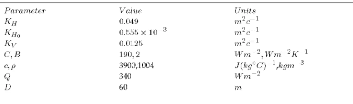
1/60and the size of the time step is calculated in an iterative way according to the formula

Figure 1. Temperature without latent heat(--y (u)= u) and t= 5.

5

,

,

2

,

o

.,

.,.,_,

~ -0.6

-,

..

.,

·10 ·11 12

"

."

.,.

'"

"

7 -6"

o

4

a

2:

,

o

_.,

-2

-,

4 -5 -5

-,

2 ·5 -10 ·11 -12 ·13

_" ·'5

·16

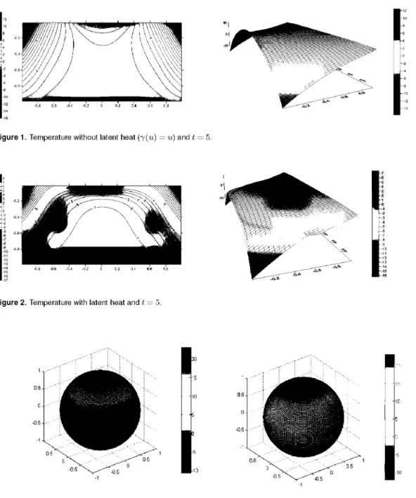
Figure 2. Temperature with latent heat and t= 5.

1'J

-5

-lD

10

20

15 0.5

10 0.5

·0.5

-0.5

-1

-5

0,5 -0.5 -10

·1

·1

Figure 3. Mean Surface Temperature without latent heat effect (leH) and with latent heat effect (right) at t= 4.

which corresponds to the presence of large regions without great abrupt temperature changes), most of the higher level lines of the sea temperature does not arrive to touch the sea surface (except, at most, sorne of them which do that around the Equator).

A numerical experiment carried out considers the delay effect. The results can be seen in Figure 4. The range of temperatures is more narrow when considering this term than without its influence. Therefore the delay term is like a memory one, whichremembers the temperature of previous time steps and, therefore, tends to smooth the spatial evolution of the temperature. In this example we have taken¡.L

=

0.5, but no latent heat, for simplicity. Another interesting feature

25 20 15 10

.--- Initial condition

- - Withoutdelay(tau=O) - - - With delay(tau=O.01) _._._. Withdelay(tau=O.1)

-0.75 -0.5 -0.25 o 0.25 0.5 0.75

sine oflatitude

Figure 4. Delay effect in the upper boundary (without latent heat effect) at t= 5 lor different values 01 the time 01 delayT.

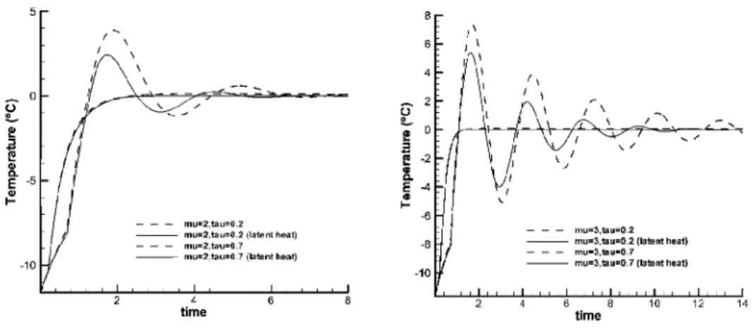
of the effect of the delay term is depicted in Figure 5 where the temperature is plotted as a function of time for the particular latitude 38° S and for different values of the parameters¡.LandT. The

results show that, in both situations, a stationary state is reached. Nevertheless, when the time of delayT is larger the solution becomes more oscillating and takes a longer time in reaching the stationary state. This effect is more evident for larger values of¡.L.This conclusion is similar to that

pointed out in [58]. Also Figure 5 reveals that the consideration of the latent heat effect give rise to less oscillating solutions.

- - - mu=3,tau=O.2

- - mu=3,tau=O.2 (Iatent heat)

- - - mu-3,tau-O.7

- - mu=3.tau=O.7 (Iatent heat)

e

.a

l!!

~

E -5

'"

1-- - - mu=2.tau=O.2

- - mu=2,tau=O.2 (Iatenl heat) - - - mu=2.tau=O.7

- - mu=2,tau=O_7 (Iatent heat)

4 time

l!!

::l

1!

-2

~

E -4

..

1--6

-8

-10

\ \

6 8

time

,

/

10 12 14

Figure 5. Temperature in the upper boundary as a lunction 01 time, with (Iulllines) and without (dashed lines) latent heat

Acknowledgements.The research of JID and LT was partialIy supported by the project MTM2008-06208 and MTM2011-26119 (DGISPI, Spain). The research of JID has received funding from the ITN FIRST of the Seventh Framework Programme of the European Community (grant agreement number 238702) and the Research Group MOMAT (Ref. 910480) supported by UCM. The research of the second author was partialIy supported by the project Consolider-Ingenio 2010 CSD2009-00065.

References

1. H. Amann, Fixed point equations and nonlinear eigenvalue problems in ordered Banach spaces, 5IAM Review, 18, No. 4 (1976) 620-709.

2. D. Arcoya, J.I. Díaz and1. TelIo. S-shaped bifurcation branch in a quasilinear multivalued model arising in Climatology, Journal of Differential Equations, 150 (1998) 215-225.

3. 1. Aubin. Nonlinear Analysis on Manifolds. Monge-Ampere Equations. Ed. Springer. 1982 4. M. Badii and J.I. Díaz, On the time periodic free boundary associated to sorne nonlinear

parabolic equations. Boundary Value Problems. Boundary Value Problems, Volume 2010, Article ID 147301, doi:10.1155/2010/147301

5. D.S. Balsara, C.W. Shu. Monotonicity preserving weighted essentialIy non-oscilIatory schemes with increasingly high order of accuracy. J Comp Phys 160 405--452, 2000.

6. K. Bhattacharya, M. Ghil, and I.1. Vulis. Internal variability of an energy-balance model with delayed albedo effects, J. Atmos. Sci., 39, 1747-1773, 1982.

7. I. Bejenaru, J.I. Díaz and LI. Vrabie. An abstract approximate controlIability result and applications to elliptic and parabolic systems with dynamic boundary conditions, Electronic

J.

Diff Eq.,2001,50,(2001), 1-19.

8. W.H. Berger, S. Burker and E. Vincent. Glacial-Holocene transition: Climate Pulsations and Sporadic Shutdown of NADW production, in Abrupt Clima tic Change - Evidence and Implications, (eds. W.H. Berger, LD. Labeyrie), Reidel Publishing Co. Dordrecht HolIand (1987).

9. R. Bermejo, J. Carpio, J.I. Díaz and 1. TelIo. Mathematical and Numerical Analysis of a Nonlinear Diffusive Climate Energy Balance Model. Mathematical and Computer Modelling, 49 (2009) 1180-1210.

10. H. Brezis, Monotonicity methods in Hilbert spaces and sorne applications to nonlinear partial differential equations, in "Contributions to Nonlinear Functional Analysis", (ZarantonelIo, E.

Ed.), Acaddemic Press New York (1971) 101-156.

11. H. Brezis, Operateurs maximaux monotones et semigroupes de contractions dans les espaces de Hilbert.North HolIand, Amsterdam (1973).

12. H. Brezis and J. I. Díaz, Mathematics and Environment, special issue of Rev. R. Acad. Cien.Serie A Matem (RACSAM), 96, N.3, 2003.

13. M.I. Budyko. The effects of solar radiation variations on the climate of the Earth, Tellus 21 (1969) 611-619.

14. M.A Cane, and S.E.Zebiak. A theory for El Niño and the Southern Oscillation, Science, 228, 1084-1087,1985.

15. A C. Casal and J. I. Díaz. On the complex Ginzburg-Landau equation with a delayed feedback. Mathematical Models and Methods in Applied Sciences, 16, 1 (2006) 1-17.

16. C. Casal, J. I. Díaz and M. Stich. Control of turbulence in oscilIatory reaction-diffusion systems through a combination of global and local feedback, Physical Review E 76, 0362091-9, 2007. 17. AC. Casal, J.I. Díaz and J.M. Vegas, Finite extinction time property for a delayed linear

problem on a manifold without boundary. Discrete and Cont. Dynam. Systems, supplement 2011. 265-271.

18. J. Casper, H. Atkins. A finite-volume high order ENO scheme for two-dimensional hyperbolic systems. J Comp Phys 106: (1993) 62-76.

19. 1.1. Crowley and G.R.North, Paleoclimatology, Oxford University Press, Oxford, 1991. 20. R.Dautray and J. I. Díaz, Lo infinitamente pequeño, lo infinitamente grande y lo infinitamente

complejo: el medio ambiente. Rev.R.Acad. Cienc. Exact. Fis. Nat., Vol. 100, N° 1,2006,13-24. 21. M.K. Davey, D.L.1. Anderson and S. Lawrence. A simulation of variability of ENSO forecast

skill: Journal of Climate, vol.9, no.1, 240-6, (1996).

23. G. Díaz and J. I. Díaz. On a stochastic parabolic PDE arising in Climatology. Rev. R. Acad. Cien.Serie A Matem, 96, N. 1, 2002, 123-128.

24. J.I. Díaz. Mathematical analysis of sorne diffusive energy balance climate models, in Mathematics, Climate and Environment,(J.I.Díaz, J.L.Lions, eds.) Masson, Paris, (1993) 28-56. 25. J. I. Díaz. Approximate controlability for sorne simple climate models. In Environment,

Economic and Their Mathematical Models(J. I. Díaz y J.L.Lions eds.), Research Notes in Applied Mathematics No 35, Masson, Paris, 29 43, 1994.

26. J. I. Díaz. ControlIability and obstruction for sorne non linear parabolic problems in Climatology. In Modelado de Sistemas en Oceanografía, Climatología y Ciencias Medio Ambientales (C.Pares and AValIe eds.) Universidad de Málaga, 43 58, 1994.

27. J. I. Díaz (Edit.), The Mathematics of Models in Climatology and Environment, ASI NATO Global Change Series I, N. 48, Springer-Verlag, Heidelberg, 1996.

28. J. I. Díaz (Edit.), Ocean Circulation and PolIution Control. A Mathematical and Numerical Inquiry, Lecture Notes, EMS Volume, Springer-Verlag 2003.

29. J. I. Díaz.Onthe von Neumann problem and the approximate controlIability of Stackelberg-Nash strategies for sorne environmental problems. Rev.R.Acad. Cien. Serie A Matem, 96, N. 3,2002, 343-356.

30. J.I. Díaz, J. Hernández,1. TelIo.Onthe multiplicity of equilibrium solutions to a nonlinear diffusion equation on a manifold arising in Climatology,

J.

Math. An. Appl. 216 (1997) 593-613. 31. J. I. Díaz, G. Hetzer. A Functional Quasilinear Reaction-Diffusion Equation Arising in Climatology. Equations aux derivees partielIes et applications. Articles dedies a J.-L. Lions, EIsevier, Paris, 461-480, (1998).

32. J.I. Díaz, G. Hetzer and1. TelIo. An energy balance model climate model with hysteresis, Nonlinear Analysis 64 (2006) 2053-2074.

33. J. I. Díaz and J.L. Lions (Eds). Environment, Economics and Their Mathematical Models. Research Notes in Applied Mathematics No 35, Masson, Paris, 1994.

34. J. I. Díaz, J. 1. Lions. On the Approximate ControlIability of Stackelberg-Nash Strategies. In, Ocean Circulation and Pollution Control. A Mathematical and Numerical Inquiry, (J. I. Díaz ed.). Lecture Notes, EMS Volume, Proceedings of the Diderot Videoconference Amsterdam-Madrid-Venice, Lecture-Notes, Springer Verlag 2003,17-28.

35. J.I. Díaz, R. Jimenez. Aplicación a la teoria no lineal de semigrupos a un operador pseudodiferencial. In Actas VII CEDYA, Univ. Granada (1984) 137-142.

36. J.I. Díaz, J.A Langa and J. Valero.Onthe asymptotic behaviour of solutions of a stochastic energy balance climate model. Physica D, 238 (2009),880-887.

37. J.I. Díaz and S. Shmarev, Langragian approach to level sets: application to a free boundary problem arising in climatology, Archive for Rational Mechanics and Analysis, 194,2009, no.1, 75-103

38. J.I. Díaz,1. TelIo. A nonlinear parabolic problem on a Riemannian manifold without boundary arising in Climatology, Collectanea Mathematica (1) 50 (1999), 19-51.

39. J. I. Díaz,1. TelIo. A 2D climate energy balance model coupled with a 3D deep ocean model. Electronic Journal of Differential Equations,Conf. 16, (2007).

40. J.I. Díaz and 1. TelIo. On aclimate model with a dynamic nonlinear diffusive boundary condition. Discrete and Continuous Dynamical Systems series S, Vol 1, N. 2, (2008), 253-262. 41. J.I. Díaz and1. TelIo. On the coupling between the deep ocean and an atmospheric balanced

climate model. Maths and Water. Monografías de la Real Academia de Ciencias Exactas, Físicas Químicas y Naturales de Zaragoza.N. 31. 67-76, (2009).

42. P.G. Drazin, D.H. Griffel. On the branching structure of diffusive climatological models,

J.

Atmos. Sci.34 (1977) 1969-1706.

43. M. Dumbser, C. Enaux,E.F.Toro. Finite volume schemes of very high order of accuracy for stiff hyperbolic balance laws. J Comp Phys 7 (8) (2008) 3971-4001.

44. A Friedman, Partial Differential Equations of Parabolic Type, Prentice-HalI, Englewood (New Jersey),1964.

45. M. Ghil and S. Childress, Topics in Geophysical Fluid Dynamics: Atmospheric Dynamics Dynamo Theory and Climate Dynamics.Springer Verlag. Applied Mathematical Sciences. 1987.

46. M. Ghil, I. Zaliapin, and S. Thompson. A delay differential model of ENSO variability: parametric instability and the distribution of extremes. Nonlin. Proc. Geophys., 15, 417-433, (2008).

48. A. Henderson-SelIers and K. McCuffie. AClimate Modelling Primer, John Wiley&Sons, Chichester (1987).

49. C. Hetzer. The structure of the principal component for semilinear diffusion equations from energy balance c1imate models,Houston Journal of Math. 16 (1990) 203-216.

50. C.Hetzer,1. TelIo.Ona reaction - diffusion system arising in Climatology.Dynamic Systems

and Applications,11 (2002) 381-402.

51. A. Hidalgo,1. TelIo. A Finite Volume Scheme for simulating the coupling between deep ocean and an atmospheric energy balance model. In the book Modern Mathematical Tools and Techniques in Capturing Complexity. Springer Series in Complexity, Springer, Berlin (2011). 239-255.

52. J. 1. Kiehl. Atmoshperic general circulation modeling, In Climate System Modeling, (Trenberth, K. E. ed.), Cambridge University Press, (1992) 319-370.

53. J. 1. Lions, R Temam and S. Wang. New formulations of the primitive equations of atmosphere and applications,Nonlinearity5, 237-288 (1992).

54. J.C,Mengel, D.A. Short, and C.R North. Seasonal snowline instability in an energy balance

model. Climate Dynamics, 2, (1988)127-131.

55. C.R North. Multiple solutions in energy balance c1imate models, Paleogeography,

Paleoclimatology, Paleoecology82, Elsevier Science Publishers BV Amsterdam, 225-235 (1990).

56. C.R North and RF. Cahalan, Predictability in a solvable stochastic c1imate model,

J.

Atmospheric Sci.38 (1982) 504513.

57. 1. Rasool,Systeme Terre,Flammarion, 1993, Paris.

58. 1. Roques, M.D. Chekroun, M. Cristofol, S. Soubeyrand, and M. Chil, Parameter estimation for energy balance models with memory,Phil. Trans. Roy. Soco A,to appear.

59. E. Sanchez-Palencia, Non-Homogeneous Media and Vibration Theory, Springer-Verlag, Berlin 1980.

60. W.D. SelIers. A global c1imatic model based on the energy balance of the earth-atmosphere system,

J.

Appl. Meteorol.8 (1969) 392-400.

61. C.W. Shu. Total-variation-diminishing time discretizations. SIAM J Sci Stat Comput 9: (1988) 1073-1084.

62. EH. Stone. A simplified radiative-dynamical model for the static stability of rotating atmospheres,

J.

Atmos. Sci. (3) 29 (1972) 405--418.

63. M-J. Suarez, ES. Schopf, A delayed action oscillator for ENSO,

J.

Atmos. Sci.,J5, 3283-3287, 1988.

64. 1. TelIo. Estabilización de soluciones para un problema parabólico con condición de contorno dinámica y difusiva. Actas del XXICEDYAjVIII CMA. Universidad de Castilla La Mancha. ISBN: 978-84-692-6473-7, (2009).

65. VA. Titarev and E.F. Toro. Finite-volume WENO schemes for three-dimensional conservation laws.

J.

Comp. Phys.201:(2004) 238-260.

66. VA. Titarev and E.F. Toro. ADER schemes for three-dimensional non-linear hyperbolic systems.

J.

Comp. Phys.204(2): (2005) 715-736.

67. E.F. Toro and A. Hidalgo. ADER finite volume schemes for nonlinear reaction-diffusion equations,Applied Numerical Mathematics59 (2009) 73-100.

68. J. von Neumann. Can we survive Technology?, Nature. (1955) (Also in John von Neumann: ColIected Works. Vol VI, Pergamon, 1966.)

69. 1. 1. Vrabie,Compactness methods for nonlinear evolutions,Pitman Longman. London. (1995). 70. RC. Watts and M. Morantine. Rapid c1imatic change and the deep ocean,Clima tic Change 16

(1990),83-97.