Dynamics of high-speed railway bridges: review of design issues and new research for lateral dynamics

1 Introduction

Traffic loads on railway bridges are a major action to be considered for evaluating the safety and functionality of structures. Not only the traffic loads are larger than for road bridges, they also may produce significant dynamic effects due to their regular spacing. Furthermore, the nature of the guided traffic on rails imposes more stringent safety requirements than for road vehicles, resulting in limitations to deck accelera-tions and deformaaccelera-tions. With the advent of faster trains in new high-speed railways and increased demands on the infrastructure the relevance of these dynamic effects has become one of the key design factors for railway bridges.

In this work we start by reviewing some of the basic features related to the dynamic response of bridges under traffic loads (section 2). Some of these features are key aspects for the design and functionality of structures in the new high speed railway lines, and have been incorporated into the recent engineering codes [3, 4, 7, 35]. The discussion here has a conceptual approach, hence the models employed will be simple in order to help in understanding the basic design issues and modelling options.

The basic solution of a moving load on a simply supported bridge [33] involves ne-glecting the non-suspended mass (wheelsets) as well as the vibrations of the suspended masses, a sufficiently approximate solution for many cases. It is easily obtained that the maximum dynamic increment over static effects for a moving load is '0 _{= 77%,}

using standard notation for railway structures engineering [34]. However significant, this increase may be easily bounded by a factor in the design codes, the so-called im-pact factor. This has been the basis of the approach followed in engineering codes up to very recently [34], until high-speed trains have arrived.

The new high-speed trains introduce a potentially much greater dynamic effect, the resonant response of the bridge from regularly spaced axle loads at speeds whose effective frequency may coincide with the fundamental frequencies of the structure. Resonance is not adequately covered by an impact coefficient and requires a dynamic analysis of the bridge.

As a result of research carried out in Europe to investigate high speed traffic ac-tions [11] the new codes for design of railway bridges take into account resonant phenomena from traffic, in the Eurocodes [3], UIC code [35] or Spanish code [7]). In addition to conservative static load models (LM71) and impact factor envelopes( ) they prescribe dynamic analyses to check resonance under certain circumstances. Fur-thermore they define a High Speed Load Model (HSLM) which provides a dynamic envelope for European high-speed trains and enables interoperability within the trans-European network [13].

In general, it is unlikely that the structural Ultimate Limit States (ULS) would be reached from dynamic traffic actions in bridges designed according to modern stan-dards. More often, the critical issues are Service Limit States (SLS) [21] such as the maximum vertical accelerations of the bridge deck. This limit for ballasted track is

amax = 3.5 m/s2 [4], in order to avoid risk of destabilization of the ballast and

observed in short span bridges, due to two reasons: the low overall mass of the bridge, and the fact that the resonant action of the axles (bogies) may be more pronounced for span lengths shorter than the vehicles.

In section 3 this paper deals with lateral dynamics of vehicles on viaducts. This proves to be a phenomenon which may be significant in some cases and for which a coupled full vehicle–structure interaction model must be employed. The interest for this study originates from the observation of significant lateral vibrations in some Eu-ropean railway bridges, with metallic open deck sections, high lateral compliance and consequently low lateral eigenfrequencies. These vibrations affect the train as well as the structure, and were studied under the auspices of UIC and ERRI [10]. The con-clusions of this work have resulted in design limits for railway bridges incorporated in the structural Eurocodes and UIC codes [4, 35].

A different type of railway structures with high lateral compliance in relative terms are the long continuous viaducts with high piers erected in some high-speed railway lines. Several such viaducts form part of the new Spanish HS lines [20]. In principle these viaducts are not affected by the conclusions of the ERRI studies cited above; however, they also have low frequencies for lateral vibration, but associated in this case with modes of very long wavelengths. In spite of the above, some uncertainties remain about the lateral response of these viaducts, being one of the objects of the present work.

Lateral oscillations may arise from self-excited causes: track alignment irregular-ities, nosing motion of the wheelsets, deck torsion specially on double track decks, lateral bending of piers, or centrifugal forces. Another obvious origin is external ac-tions, mainly cross winds and earthquakes. It becomes important to evaluate the safe running conditions under these circumstances, such as the characteristic wind curves (CWC) [14].

In this work we propose coupled train–bridge dynamic interaction models for eval-uating the running safety of trains over railway viaducts. The models for these prob-lems include the following ingredients [39]: 1) dynamic model for structure subsys-tem; 2) dynamic model for the vehicle subsyssubsys-tem; 3) description of track irregularity profiles; 4) wheel-rail contact models; and 5) adequate numerical solution algorithms for the equations.

Most of the existing approaches to this problem assume linear models both for the structure subsystem and also for the vehicle multibody system [30, 36–40]. In these models quadratic velocity terms, such as gyroscopic effects, are also neglected. Some approaches which consider nonlinear effects for vehicle and structures have been proposed by [31, 32], and in [22], where a linear model is used for the vehicle with additional gyroscopic terms included for the wheelsets.

this work Abaqus [28] finite element framework has been used. Both subsystems (bridge and vehicles) are described with coordinates in absolute reference frames, as opposed to alternative approaches which describe the multibody system with coor-dinates relative to the base bridge motion. This facilitates the full consideration of nonlinear inertia terms, without introducing additional difficulties for the structural mechanical behavior [27].

Contrary to the majority of existing models for train–bridge dynamic interaction, the formulation described here is capable of full consideration of geometrical and ma-terial nonlinearities both in the structural subsystem (bridge) and in the multibody subsystem (vehicle). The approach for wheel–rail geometrical interaction and me-chanical contact model is fully nonlinear as well, not being limited neither to constant conicity assumptions nor to linearized elastic contact forces. The particular model reported in this work involves some simplifying assumptions that will be described below.

In the rest of this paper we discuss first the dynamic response of bridges in section 2, reviewing the“impact”action of moving loads, resonance, and models available for dynamic analysis. Following, in section 3 we describe the models for lateral dynamics of vehicles on viaducts. Two representative applications will be presented in section 4. Finally, some concluding remarks are summarised in section 5.

2 Dynamic response of bridges

2.1 Dynamic response to moving load

The solution to a moving load on a simply supported bridge is well established and available in closed form under certain assumptions. However, it is interesting to review for several reasons. Firstly it provides a basis for defining a dynamic factor (or impact factor) for design. Additionally, the closed form solution helps to identify clearly the characteristics of the dynamic behavior.

From the dynamic equation of vibration of a beam, the solution may be performed with a modal analysis [33], in which we shall take only the fundamental mode of vibration of frequencyf0 = !0/2⇡ (further down we shall consider the implications

of taking more modes). For a load at constant speed v thewavelength is defined as

=v/f0. Additionally, for a bridge of spanLa non-dimensional parameter↵for the

load velocity may be defined as:

↵ = 2L =

v

2f0L

. (1)

The displacement time history response at the center of the span, in terms of the maximum static response ys = P L3/48EI ⇡ 2P L3/⇡4EI and considering some simplifications valid for small damping (⇣ _⌧1) is:

y(t) = ys 1 ↵2

⇥

sin (↵!0t) ↵e ⇣!0tsin (!0t)

⇤

where the first term within the brackets is due to the excitation from the external load and the second to the free vibration of the bridge.

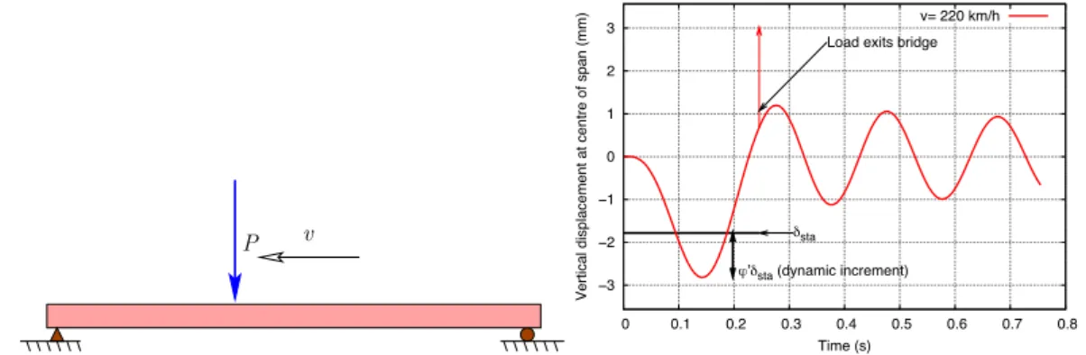
Figure 1 shows an application for aL= 15m simply supported beam-type bridge. The computed dynamic increment at 220 km/h, with 2% structural damping, is'0 = 59%. The critical velocity, for obtaining a maximum dynamic increment, would be in this case 333 km/h, corresponding to an increase of '0 _{= 77%with no damping.}

In real bridges, additional dynamic effects must be considered from the irregularities of tracks and wheels (represented by parameter'00_{in UIC standard railway structures}

engineering notation [34]). However, these are generally of less importance for the bridges: in this case they would only amount up to an additional0.5'00 = 2%dynamic increment for a well maintained track [34].

v P −3 −2 −1 0 1 2 3

0 0.1 0.2 0.3 0.4 0.5 0.6 0.7 0.8

Vertical displacement at centre of span (mm)

Time (s) Load exits bridge

δsta

ϕ’δsta (dynamic increment)

v= 220 km/h

Figure 1: Dynamic increment for moving load on simply supportedL= 15 mbridge, from catalog of ERRI D214 [11], withv = 220 km/hand damping⇣ = 0.02.

The solution (2) is valid during the time the load is on the bridge, under this as-sumption the maximum ydyn in terms of t may be computed (for very fast moving

loads when the maximum is reached after the load exits the bridge the response is lower). For the most unfavourable case without damping (⇣ = 0) the maximum is attained fory˙= 0 ) !0t = ₁2n_↵⇡, with the result

ydyn

ys

= 1

1 ↵2



sin

✓

↵ 1 ↵2⇡

◆

↵ sin

✓

1 1 ↵2⇡

◆

. (3)

This expression yields an envelope of the dynamic factor with respect to the non-dimensional parameter↵, plotted in figure 2. This envelope curve shows a maximum response for a critical value of↵c (and associated critical speed,vc = 2↵cf0L):

↵c = 0.617 )

✓

ydyn

ys

◆

max

= (1+'0_dyn)_max= 1.768. (4)

In figure 2 the code envelope'0UICis also plotted for comparison, which proves to be

sufficiently conservative.

As an example, for the bridges in the D214 ERRI study [11] the maxima of'0

dyn

correspond to vc = 333 km/h for the L = 15 m bridge and vc = 356 km/h for

1 1.2 1.4 1.6 1.8 2 2.2 2.4

0.1 0.2 0.3 0.4 0.5 0.6 0.7 0.8

impact factor (1+

ϕ

’)

α=v/(2f₀ L)

moving load on simply supported beam

max (0.617, 1.768)

max (0.760, 2.325) 1+ϕ’_dyn

1+ϕ’_UIC

Figure 2: Envelopes of impact coefficient;'0

dynfrom analytic solution (3) and'0UIC

from [35]. The various lobes in '0

dyn correspond to slow loads for which the beam

performs more than one full oscillation during passage.

2.2 Dynamic analysis with moving loads

Resonance in bridges.— In order to motivate the need for more complete dynamic analysis, figure 3 shows some measured results for a bridge in the Madrid-Sevilla HS line, from an AVE S100 (ALSTHOM) train at 220 km/h. The bridge consists of a

Figure 3: Measured vertical displacement at center of simply-supported span in viaduct over Tajo river, Madrid-Sevilla high-speed line, together with results of simu-lation with moving load model [9]. AVE S-100 single unit train at 220 km/h

sequence of simply supported spans with L = 38 m. The measured and computed

results show an impact coefficient of approximately (1 +'0_{) = 2.0, measured with}

P1

v

2 3 4 5 6 7

P P P P P P

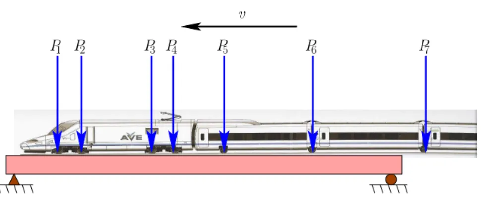
Figure 4: Load sequence from HS train for moving load dynamic analysis, showing AVE S-102 (Talgo) HS train with regularly spaced single axles.

effect is not so much a problem for the Ultimate Limit State (ULS) of the bridge, which in this case is covered by the safety margins embedded in the normative static vertical load envelope LM71 and the impact coefficient employed for the design [3]. However, in this case the functionality of the bridge was impaired: vibrations induced in the catenary posts proved to be excessive and these had to be relocated into new positions. In other cases the resonant dynamic effects may be even of much greater magnitude, and must be therefore avoided in the design of bridges.

Models for analysis.— The Impact factor is derived from moving load envelopes for analysis of real trains at conventional speeds (i.e.  200 km/h). It does not cover

resonant effects, which may be much greater than moving load effects; in order to consider resonance an impact factor approach would be either unsafe or excessively conservative. For circumstances in which there is a possibility of resonance it is neces-sary to perform a dynamic analysis of the whole train taking into account the complete load sequence (figure 4). In order to discuss these concepts, we shall consider in what follows models for the simplest case, a straight beam subject only to vertical bending, for which the differential equation governing the dynamics is

mu¨+ (EI u00)00 =p(x, t) = N

X

k=1

Pkh (x+dk vt)i, (5)

for a train with N concentrated axle loadsPk with offsetsdk, wherexis the longitu-dinal coordinate, u(x)the beam vertical displacements, m the mass per unit length,

and (·)is the Dirac delta function. The bracketsh·ihave the meaningh (⇠)i= (⇠) if 0 < ⇠ < L (load within bridge) or 0 otherwise. Superposed dots ( ˙_•) represent time derivatives and primes (_•0_{) derivatives with respect to x. This equation may}

be generalized for arbitrary structures either with 3D beams, torsional effects, shear deformation, or more general continuum-type descriptions. In particular, torsion is added straightforwardly to the above equation.

can be performed analytically through modal analysis, obtaining uncoupled modal equations for the amplitude of vibration of each mode [6]. Considering mode shapes

i(x)and associated circular frequencies!i:

Miy¨i+2⇣i!iMiy˙i +!i2Miyi = N

X

k=1

Pkh i(x+dk vt)i, (6)

where yi is the amplitude for mode i, Mi is the corresponding modal mass and ⇣i the damping ratio. These equations may be integrated in time by direct numerical algorithms (either coded directly or available within finite element software).

A more general procedure is to employ finite element (FE) software for the dis-cretization of the dynamic equations in space, enabling solution of fully 3D problems. The only feature which is special for these dynamic problem, as compared to other structural dynamics problems, is the adequate definition of the actions from the mov-ing loads, which needs an ad-hoc preprocessmov-ing. As a result of FE discretization the following matrix system of ordinary differential equations is obtained

Mu¨+Cu˙ +Ku=f(t), (7)

whereM,CandKare respectively the mass, damping and stiffness matrices andf(t) the load vector obtained from the moving loads. At this point within FE software it may be chosen to do adirect time integrationof the coupled equations (7) with a nu-merical scheme, or to perform amodal analysisof the discretised system and obtain numerical mode shapes and frequencies. These will then be available as uncoupled equations identical to (6) and may be integrated in time individually. The modal anal-ysis option has several advantages. The number of modes to consider can be chosen thus avoiding high-frequency components from higher modes, which are not signif-icant for the bridge response. Moreover, the solution is generally much faster. The alternative approach of performing a direct time integration of the complete system provides a more general method, which may be necessary in some cases, for instance to consider nonlinear effects such as contacts.

Example with enhanced impact.— Following we discuss an application, solved with a dynamic moving load analysis. It serves as an example of a case with an enhanced impact effect with respect to the single moving load solution in section 2.1, due to a phenomenon which may be termed“repeated impact”. Figure 5 shows the case of an articulated multiple unit train (MU) [29] at the critical moving load velocity (↵c = 0.617, vc = 353 km/h), together with the quasi-static response neglecting inertial vibration. The impact factor obtained is(1 +'0) = 2.45, clearly larger than

that for a moving load (figure 2). We remark the response in this case is not a case of resonance, but does represent a case for which the simple moving load coefficient is not sufficient.

 



 

            

0 10 20 30 40 50 60 70 80 90 100 110 5

0 5

x[m]

[mm]

quasi-static moving loads

Figure 5: Response for v = 353 km/hload model for articulated MU AB 2D [29], 5 coach unit with individual axle loads P = 21.5 t; vertical displacements at

mid-span for L = 20 m bridge from ERRI D214 [11], considering moving loads; The horizontal axis represents the distance x = vt allowing synchronized comparison at

different speeds.

loads due to the stiffness of rail, railpads and ballast [12] as they attain the deck of the bridge. This distribution may have some significance for short bridges, as compared to the consideration of concentrated point loads [3]. A reasonable assumption for usual track stiffness is to consider a 1

4 – 1 2 –

1

4 distribution on 3 consecutive sleepers

sep-arated 0.60m. Figure 6 shows a representative example, the maximum acceleration envelope in the bridge deck as a function of train speed for a 10 m span bridge and a reference MU load model, with a reduction of approximately10% in dynamic effects at the critical speed.

Number of modes to consider.— An issue which may be of importance is the num-ber of modes to consider in the modal analysis. Some indications to this purpose are given in the Eurocode [4] for checking accelerations on the bridge deck. For a dis-placement analysis of a simply supported beam, it may be generally carried out with only the first (fundamental) mode. Acceleration analysis or the extraction of stresses or sectional resultants will often require more modes to be considered.

As an example, we present comparative results for the case of the ERRI D214

L = 30 m bridge under the ICE3 HS train in figure 7. The fundamental (first sym-metric) mode frequency is in this casef1 = 3 Hz, and the second symmetric mode is

f3 = 27 Hz(the 2ndmode is skew-symmetric and has no influence on mid-span

                 

80 100 120 140 160 180 200 220 240 260 280 300 0

1 2 3 4

v[km/h]

Max . accel er at ion [m / s 2]

Distributed loads (1 4

-1 2

-1 4)

Concentrated point loads

Figure 6: Envelopes for maximum accelerations showing the effect of track load dis-tribution; reference load model for articulated MU AB 1D [29], 5 ⇥ 5 coach units with individual axle loadsP = 21.5 t. Simply supported bridgeL = 10m, m = 12 t/m,f0 = 12.464Hz,⇣ = 2.2%.

0 1 2 3 4 5

20 10 0 10 20 time [s] mid-span de fle ction

[mm] 1 symm. mode_{2 symm modes}

0 1 2 3 4 5

5 0 5 time [s] mid-span ac ce le ration [m / s 2]

1 symm. mode 2 symm modes

Figure 7: Influence of number of modes for simple bridge, on displacements and accelerations. ICE3 HS train at v = 268 km/h on L = 30 m bridge from ERRI D214 [11]

yield only minor increases to these accelerations.

2.3 Models with vehicle-structure interaction

M, J

L

d d

d

M M

G

M_w K_s,c_s K_s,c_s

K_p,c_p b,Jb K_p,c_p b,Jb

M_w

td Bd

eB

Figure 8: Schematic representation of models for vehicle-bridge interaction

of the bridge to be transferred to the vehicles, and consequently will predict lower vibrations on the bridge.

Vehicle subsystems may be generally considered as rigid bodies, with masses for wheelsetsMw, bogiesMb and Vehicle boxM, and concentrated springs and dampers, as shown in figure 8. Models for vertical dynamics need include only vertical trans-lation degrees of freedom and pitch rotations for vehicle body or bogies, resulting in relatively simple multibody models. Models for lateral dynamics include transver-sal displacement and generally also roll and yaw rotations. These need complete 3D descriptions and should be handled with general multibody models, either linear or nonlinear, as described in section 3.

2.3.1 Simplified Interaction Model

Often full vehicle-bridge interaction models such as shown in figure 8 are not required, as some parts of the vehicle will not interact with the bridge, depending on the fre-quencies of vibration. Bodies with frefre-quencies which are very low with respect to the bridge will not be excited by the bridge motion and behave as constant moving loads. Bodies with frequencies which are much higher will behave as added masses.

For railway passenger vehicles under vertical motion one can identify three ba-sic characteristic frequencies for vertical vibration of the vehicle: 1) vibration of wheelsets considering Hertz contact with the rails, in the order of 100 Hz; 2) vi-bration of bogies on the primary suspension, in the order of 4 Hz; 3) vivi-bration of the vehicle box, in the order of 1 Hz. In practice, the types of bridges which show greater dynamic vibrations have fundamental frequencies in the order of 3 to 7 Hz, hence the interaction will provide mainly from bogie masses and primary suspensions. Wheelset masses behave (from the point of view of bridge dynamics) as rigidly attached to rails, and vehicle box masses as moving loads of fixed value.

interaction elements (one per wheelset, suspended mass + moving load). Under these

Figure 9: Simplified models for vehicle-bridge interaction including suspended bogie masses and primary suspension

assumptions, the equations for each mode of vibration ( i= 1. . .n, with amplitudes yi) are (details in [9]):

Mi y¨i+Ciy˙i+Kiyi = k

X

j=1

⌦

i dj_rel

↵

pj +mj_b z¨j , (8)

and for each interaction element (zj = 1. . . k):

mj_bz¨j +kj

"

zj

n

X

i=1

yi

⌦

i(dj_rel)↵

#

+cj

"

˙

zj

n

X

i=1

˙

yi

⌦

i(dj_rel)↵ n

X

i=1

yiv

⌦ ₀

i(d j

rel)

↵#

= 0. (9)

These equations are simple to implement and represent only a minor extension to the moving load modal analysis equations (6), with very small computational cost.

Reduction in predicted dynamic effects from consideration of interaction more rel-evant in short bridges and with frequencies of the same order as that of the primary suspension, and for critical resonant velocities. As a representative example we show in figure 10 the results as compared to moving load models. The case corresponds to a CAF articulated MU train, whose primary suspension frequency is f1 = 5.97

Hz on a L = 20 m bridge with fundamental frequency f0 = 4 Hz. The maximum

deck accelerations obtained for the critical speed v = 280km/h are 10.9 m/s2 _with

moving loads and 7.8m/s2 _{with interaction, a reduction of ⇡ 40%. The Envelope of}

maxima obtained with respect to train speed shows that the reduction obtained with vehicle interaction is relevant for critical resonant velocities, but is not significant for non resonant scenarios.

3 Lateral dynamics of vehicles on bridges

3.1 General features of model

    

 

           

0 0.5 1 1.5 2 2.5 3 10

0 10

time [s]

mid-span

ac

ce

le

ration

[m

/

s

2 ]

moving loads interaction

100 150 200 250 300 0

5 10

v[km/h]

Max

.

accel

er

at

ion

[m

/

s

2 ]

moving loads interaction

Figure 10: Accelerations obtained with moving loads and with interaction with pri-mary suspension: L = 20m bridge ERRI D214 [11], f0 = 4 Hz, ⇣ = 1%; CAF

TEMD train, primary suspension frequencyf1 = 5.97Hz. Time history for resonant

critical velocityv = 280km/h (top) and envelope as a function of velocity (bottom).

vehicle-structure models, which must take into account such features as nosing mo-tion of wheelsets on the rails as well as track alignment irregularities. These features give rise to substantially more complex models than those used for vertical dynamics described in the previous section.

In this work a fully nonlinear coupled model is proposed for the lateral dynamic analysis of vehicles on viaducts. Vehicles are considered as three-dimensional multi-body systems, and the bridge structure is modeled by means of finite elements. The model is developed in a general and modular way so that it may be easily implemented within an existing finite element analysis software with multibody capabilities. For this work Abaqus [28] finite element framework has been used. Both subsystems (bridge and vehicles) are described with coordinates in absolute reference frames, as opposed to alternative approaches which describe the multibody system with coordi-nates relative to the bridge motion at the base of the vehicle. This facilitates the full consideration of nonlinear inertia terms, without introducing additional difficulties for the structural mechanical behavior [27].

A key aspect to address is the contact interface between bridge and vehicle, for which several approaches could be followed:

1. A perfectly guided predefined path for the vehicle wheelsets, for the more direct and simplest models; in these contact points between wheels and rails share position and velocity. An assumed hunting movement can be introduced as a prescribed motion of wheelsets [8, 30, 36, 39].

2. Linear models for taking into account relative motion between wheelset and track; these rely on the classical assumption of constant conicity in wheel and rail profiles and simplified contact [37, 38, 40].

3. Nonlinear models with more detailed treatment of wheel to rail contact, such as proposed in [22, 32].

In this work we follow the last option, including a fully nonlinear wheel–rail inter-action, based on the elastic contact forces approach [25]. The approach for contact point determination at each wheel may be completely general, however the model here reported employs a contact point determination based on a pre-computed geo-metric lookup table. A single hertzian contact point [15] is considered at each wheel. The tangential contact is solved by the FastSim algorithm [17]. Following the basic features of the model are summarized. A more detailed description may be found in [2].

3.2 Kinematics of wheelset and track

The wheelsets are considered as rigid bodies, within the vehicle multibody subsys-tem. The bridge deck cross sections are also assumed to be rigid within the structural finite element model, i.e. no distortion of the plane cross section is considered. This assumption is automatically enforced by standard 3D beam-type finite elements. How-ever, both vehicle and bridge can undergo large displacements and rotations. In order to establish the contact interface with sufficient precision a detailed description of the positions and velocities of the wheel and rail points is required, whose key concepts are summarised below. A more general description of multibody kinematics may be found in [23] or more specifically for railway applications in [24, 26].

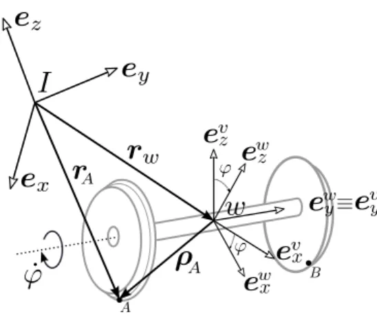
Wheelset kinematics.— The position of a wheel point A, such as the wheel-rail

contact, at a certain time instant, is defined by (Figure 11)

rA=rw+⇢A=rw +⇤w⇢¯A, (10)

whererwis the position vector of the wheelset center of mass,⇢Athe relative position of the contact point A, ⇢¯A the convective vector referred to the body reference sys-tem {w, ew

Figure 11: Reference frames and vectors for wheelset kinematics: the inertial refer-ence frame {I, ei}; the body reference frame {w, ewi }; and an intermediate frame which does not consider wheelset spin{w, ev

i}

wheelset. We shall consider that the spin of the wheelset is a given rate '˙. It is ad-vantageous to employ an intermediate reference frame{w, ev

i}which does not inherit this spin, as in this frame the contact point of one wheel will be a constant vector⇢˜A.

Considering a given parametrization✓v for rotations (Euler angles, Euler parame-ters. . . ), the angular velocity!w can be expressed in general as

!w =!'+!v =!'+G✓˙v, (11)

whereGis a non-constant matrix operator whose structure depends on the choice of parametrization and whose coefficients depend on the rotation coordinates✓v.

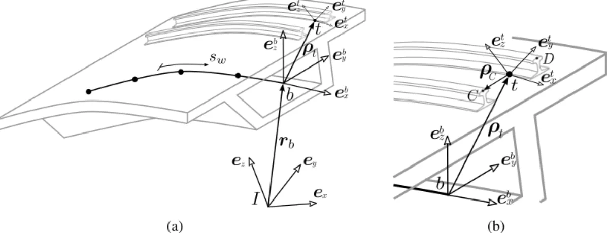
Track kinematics.— We consider a bridge deck section at a position on the deck defined by the longitudinal coordinate sw (Figure 12). The position vector of a point

C on the rail, in a similar way as for the wheelset, may be expressed as

rC =rb+⇤b⇢˜t+⇤t⇢¯C (12)

whererbdefines the position of the reference point on the deck section. Two reference frames are used for the track: the bridge section reference system b, eb

i which is attached to the deck section at pointb, and the track reference frame{t, et

i}attached to the track point t located at the mid point between the top of both rails and at the

same deck section. ⇤b and⇤t are, respectively, the rotation tensors that relate both reference systems and the inertial frame.

The position of deck section reference pointrb is obtained by interpolation of the finite element nodal coordinates along the bridge deck,

rb =rb0+Td(sw)qB, (13)

(a) (b)

Figure 12: Reference frames and vectors for track kinematics: intermediate frame attached to the deck section b, eb

i and the track coordinate system{t, eti}

initial position vector of the deck section. In the same way, rotation parameters will be interpolated as

✓b =✓b0+T✓(sw)qB, (14)

where T✓(sw) is the rotations interpolation operator and ✓b0 the initial values of

ro-tation parameters. The above expression contains the implicit assumption of small rotations for the bridge deck, for which case the rotation vectors may be interpolated linearly, as opposed to finite rotations which would require an interpolation of the exponential mapping.

3.3 Wheelset-track interaction

In order to compute the contact forces between wheels and rails the problem may be split in three consecutive stages:

1. Contact geometry: the main geometric variables involved in the problem are computed;

2. Normal contact: the dimensions and shape of the contact area and the normal stress distribution are determined;

3. Tangential contact: the resultant forces and moment of the tangential stresses, which appear as a consequence of the rolling contact, are obtained.

Assuming that the material properties of wheel and rail are the same (material sym-metry), the normal and tangential problems may be considered uncoupled [19] and solved consecutively after the determination of the geometric variables.

the plane cross section of the bridge (i.e. perpendicular to vectoreb

x, Figure 12). Under this assumption, yaw rotation is neglected when assessing the main geometric vari-ables involved in the wheel-rail contact. For a high-speed train running on a straight track, which is the case considered in this work, yaw rotation remains small and this approximation may be considered reasonable. Under this assumption the relative dis-placements between the wheelset and the track may be defined by 3 coordinates, the lateral and vertical relative displacements ( yw and zw respectively) and the rela-tive rotation within the cross section w. Furthermore, two additional hypotheses are assumed:

1. The contact between the wheel and the rail occurs at only one point (area) at each wheel;

2. No separation occurs between wheels and rails.

Under these hypotheses, the relative vertical displacement zˇw and rotation ˇw, due to purely geometric considerations, can be computed as a function of the relative lateral displacement yw for given wheel and rail profiles (in Figure 13 these are plotted for the S1002 wheel and UIC60 rail profiles):

ˇ

zw = zˇw( yw), (15a)

ˇ_{w =} ˇ_{w( yw). (15b)}

The relative coordinates zˇw and ˇw, the contact angles (Figure 14), rolling radii r and transversal curvatures at both wheels are stored in a lookup table, from

which these geometric variables will be obtained by interpolation for a given value of

yw.

8 6 4 2 0 2 4 6 8

10 5 0 5 10

Dyw[mm]

ˇ_Dz[mm],w

ˇ

Dyw

[mrad]

ˇ Dzw

ˇ Dyw

Figure 13: Compatible relative vertical motion zˇw and rotation ˇw for S1002 wheel profile and UIC60 rail

Figure 14: Contact reference frame

{C, ec

i}and definition of angle at con-tact point of one wheel

major and minor semiaxesa andb respectively. The normal stress distribution is

as-sumed to be an ellipsoid whose resultant is the normal contact forceN. The wheel and

rail curvatures at the contact point may be computed as a function of yw as shown above. From these one may compute their mechanical properties, the resultant normal forceN, the ellipse semiaxesaandband the normal stress distribution, according to

Hertz theory.

The solution for the tangential contact forces at each wheel contact is a complex nonlinear problem for which a reference solution may taken as Kalker’s exact three-dimensional rolling contact theory [18]. The coupled simulation of trains on bridges will require numerous evaluations, at each time-step and each wheel of the train. In order to bring down computational costs to reasonable bounds while maintaining suf-ficient precision for the simulations, the simplified FastSim algorithm [17] is used here, involving a compromise between accuracy and computational cost. The FastSim method has been implemented by the authors as a user subroutine within the Abaqus software employed [28] (further details in [1]).

For a given friction coefficientµ, the input variables for evaluation of tangential

rolling forces are the the normal stress distribution, the ellipse semiaxes and the creep-ages, defined as⇠ = [⇠x,⇠y,⇠r]T which are defined as:

⇠_{x,y} =

(vA vC)·ec_{x,y}

v ⇠r =

(!w !t)·ecz

v , (16)

withvthe wheelset longitudinal velocity. The FastSim model involves a discretisation

in strips within the contact ellipse and integration along each strip, as shown in Figure 15. In this figure a representative case for distribution of tangential stresses is shown also.

58

3.4. Problema tangencial

de forma matem´atica como:

⌧

(

x

+

x

, y

) = ˆ

⌧

(

x

+

x

, y

)

si

|

⌧

ˆ

(

x

+

x

, y

)

|

< µ

(

x

+

x

, y

)

⌧

(

x

+

x

, y

) =

µ

(

x

+

x

, y

)

ˆ

⌧

(

x

+

x

, y

)

|

ˆ

⌧

(

x

+

x

, y

)

|

si

_|

⌧

ˆ

(

x

+

x

, y

)

|

µ

(

x

+

x

, y

)

,

(3.30)

Por tanto, si no existe deslizamiento, la tensi´on hipot´etica calculada se da

por v´alida, en caso contrario, el valor m´aximo de la tensi´on tangencial ser´a el

definido por la Ley de Coulomb, y la direcci´on ser´a la de la tensi´on hipot´etica.

Partiendo de la Ecuaci´on 3.29, y haciendo uso de la Ecuaci´on 3.30, es

posible obtener la distribuci´on de tensiones tangenciales

en toda la

elipse de contacto. Para cubrir de una forma discreta la totalidad de la elipse,

es necesario discretizar, adem´as de en la direcci´on

, en la direcci´on

. Para

llevar a cabo la discretizaci´on se toma un n´

umero de divisiones seg´

un la

direcci´on

(

), y otro seg´

un la

(

). Valores razonables son

y

pyc = 20

, que es lo adoptado para este trabajo

2

_{. Una vez elegido el n´}

_umero

de franjas

, el valor del ancho de cada una en esa direcci´on es

2b/pyc

. Cada franja de ancho

tiene una longitud variable, por lo que los

incrementos

ser´an distintos para cada franja y depender´an del valor

de

los puntos medios de cada rect´angulo, siendo

(posteriormente se explica el porqu´e del signo menos). Ver Figura 3.21.

Figura 3.21.Elipse de contacto discretizada. En el centro de cada rect´angulo de la discretizaci´on se

obtendr´an los valores de las tensiones tangenciales seg´un las dos direcciones locales, mediante FastSim,

lo que permitir´a conocer una distribuci´on de tensiones en toda la huella.

Suponiendo conocida la tensi´on

, mediante la Ecuaci´on 3.29 es

posible determinar el valor de la tensi´on

(Figura 3.22).

Inicial-2_{La elecci´on p}

xc y pyc debe ser un compromiso entre la precisi´on y la eficiencia del

c´alculo.

Figure 15: Discretisation of contact ellipse with FastSim and evaluation of tangential forces in rail-wheel contact

The resultants of the shear stress distribution at a pointAare the forcesTx andTy and the momentMz whose directions are, respectively,ecx,ecy andecz:

fC,A =Txecx+Tyecy +Necz, (17a)

Finally, in order to establish the geometric compatibility between wheels and rails set in equation (15), two constraint equations are defined at every wheelset:

{ w}=

⇢

zw zˇw( yw) w ˇw( yw) =

⇢

0

0 . (18)

These constraints are enforced through a penalty method, with coefficients computed by a linearization of the Hertz contact.

3.4 Vehicle-bridge system dynamics

Considering wheelset contact forces and moments from (17) (fC,mC), applied ex-ternal loads(fE,mE)and loads transmitted by the suspension systems(fS,mS), the Newton-Euler equations for a single wheelset can be written as

mr¨w+fS =fE +fC, (19a)

J!˙w+!w ⇥(J!w) +mS =mE+mC, (19b)

beingmthe mass andJ the inertia tensor for the wheelset.

For a general case of parametrization of rotations Gas defined in (11), equation (19b) can be expressed as

JG✓¨v +JG˙✓˙v +!w⇥(J!w)

| {z }

mQ

+mS =mE +mC, (20)

where the quadratic velocity terms have been included within the term mQ. The

wheelset dynamic set of equations (19) may be assembled as

Mwq¨w+Fw_I =Fw_E+Fw_C, (21)

being

[Mw] =



m1 0

0 J G , {q w

}=⇥rw ✓v

⇤T

, (22)

and similarlyFw

I,FwE,FwC the assembled force vectors.

Employing standard multibody dynamics models for the remaining of the vehicle, these equations may be assembled into a full system of equations for the complete vehicle. On the other hand, the discretised equations for the bridge structural dynamics may be obtained following standard finite element procedures, and expressed in a similar fashion. Finally, the two nonlinear coupled sets of differential equations may be written as

MBq¨B+FB_I =FB_E+FB_C, (23a)

MV q¨V +FV_I =FV_E+FV_C, (23b)

where the superscript B is referred to the bridge andV to the vehicles, (FB

I ,FVI ) are the internal force vectors, (FB

vectors. For the bridge the internal force vector corresponds to the forces and moments which appear as a consequence of the structural deformation. In the case of vehicles, forces and moments produced by suspension systems and quadratic velocity terms are included in this vector.

The interaction forces and moments of every wheelset are arranged in FV C. For the bridge, interaction forces applied on the track are extrapolated to the correspond-ing nodal coordinates of finite element model and assembled in FB

C. These vectors establish the coupling between the equations of both subsystems.

The nonlinear set of differential equations (23) may be solved in time using an implicit integration method. In this work the HHT-↵ algorithm [16] has been used, included in Abaqus software [28]. This method has a good stability and robustness for the coupled problems described, and includes an inherent tunable numerical damping for the high frequency noise. The constraints inherent to the multibody subsystem are solved efficiently with augmented lagrangian procedures.

4 Applications in lateral dynamics

4.1 Vehicle running on continuous deck bridge

Two representative applications of the proposed models will be shown. First the re-sponse of a representative high-speed vehicle when it crosses over a multi-span bridge with continuous deck is analyzed. The mechanical data for the vehicle are detailed in Appendix A.

The structure is a single track continuous bridge consisting of six equal spans of

L = 50m each. The bridge is supported on two end abutments and five intermediate piers. Torsional rotation is allowed at the piers but constrained at the abutments. The deck cross section properties are uniform along the bridge length, see Appendix A. The first lateral and vertical bending eigenfrequencies are equal, of value2.18Hz; the first torsion eigenfrequency is1.10Hz. Euler-Bernoulli beam elements of1m length with linear elastic behaviour have been used.

The vehicle runs at a constant velocity of100 km/h, with a lateral transient wind

gust load defined by a chinese hat function [5] applied, with maximum valueFmax = 270 kN and gust duration ⌧ = 0.1s (Figure 16). This load is applied on the vehicle car-body along y direction (transversal) when the last wheelset of the vehicle enters

the bridge.

In Figure 17 the lateral response of the last wheelset of the vehicle when it crosses the bridge is shown, compared with the case for a perfectly rigid track (i.e. no struc-ture). It can be seen that wheel flanges contact the lateral part of rail heads, the limits are indicated in the graph with dotted lines. We remark that for assessment of these running safety scenarios a nonlinear model such as proposed here is essential, as linear models cannot reproduce wheel–flange impacts.

0 0.2 0.4 0.6 0.8 1

Fmax

t[s]

F

(

t

)

Figure 16: Lateral force history on vehicle car-body: wind gust load corresponding to a“chinese hat”function

0 100 200 300 400

5 0 5

Wheel flange contact

x[m]

D

yw

[mm]

With structure Without structure

Figure 17: Lateral response of last wheelset; dotted lines indicate limit for wheel flange contact

0 100 200 300 400

50 0 50 100

x[m] yc

[mm]

With structure Without structure

Figure 18: Lateral response of the car-body under an applied wind gust load

0 100 200 300 400

10 0 10

x[m] Ty

[kN]

With structure Without structure

Figure 19: Tangential contact forces at the left wheel of the last wheelset, showing peaks for wheel–flange contact

tangential force Ty time history. This force is expressed at each instant in the local tangent plane to the whee contact (i.e. frame {C, ec

i}) of the left wheel of the last vehicle wheelset; it cannot be interpreted as a lateral load.

Figure 17 shows a significantly different response for wheelset displacements when the structure flexibility is taken into account: not only in terms of amplitude of oscil-lations, but also of frequency. A similar remark can be made for the car-body dis-placements, Figure 18. Moreover, contact forces in Figure 19 exhibit peaks which correspond to the flange impacts, these impacts differ significantly in both models.

4.2 Application for viaduct “Arroyo las Piedras”

of this viaduct is0.313Hz and corresponds to a lateral deformation mode (figure 20). More complete details of the structure may be found in [20].

Figure 20: Viaducto “Arroyo las Piedras” in C´ordoba–M´alaga HS line: first mode of vibration0.313Hz

As described above, the model for the viaduct is based on 3D beams with appro-priate kinematic constraints. The Rayleigh method has been used for the damping matrix of the structure subsystem, with0.5%damping centered in the two first natural frequencies. The train that has been used in the calculations is an approximation of the Siemens ICE 3 composed of 8 cars, each of24.775m length. The ICE3 is a multiple unit (distributed power) train, and all cars are supposed to have the same geometrical and mechanical properties.

Calculations have been carried out for train speeds of250,300and350km/h, with several models:

(1) Bridge only model with moving loads, consisting only of the bridge dynamic subsystem, with the vehicle wheelsets simplified as moving loads of fixed mag-nitude. This amounts to neglecting the dynamic effects of vehicle vibration, and serves as a basic result with which to compare the influence of the vehicle vi-bration on the results. It also serves the purpose of obtaining a so-calledvirtual pathfor the wheelsets of the vehicles, which can be later applied to these in a sequential approach to the vehicle-bridge dynamics: the bridge history of dis-placements is obtained in a first step, and these histories are then applied in a second step to the vehicle wheelsets to obtain the response of the train.

(2) Vehicle model, consisting only of the vehicle subsystem, in two different sce-narios:

(a) Vehicle on rigid track (i.e. no bridge) with prescribed profiles of irreg-ularities. This model will enable to compare the influence of the bridge deformation on the vibrations of the vehicle.

(3) Bridge-Vehicle model, performing the calculation for the global coupled sys-tem with wheel-rail contact interaction. In this case, two scenarios have been considered:

(a) Model with interaction but without track irregularities (b) Model with interaction and with track irregularities

Following we show only the results for train speed of v = 350 km/h, as they correspond to the greatest effects. Firstly we present results for the deformation of the bridge deck: displacements and rotations at the center of span 11, corresponding to the tallest pier, are shown in figure 21. These correspond to the three different scenarios defined above, the cases enumerated as 1, 3a and 3b. It may be clearly seen that the influence of the vehicle vibration and of the track irregularities on the bridge deformation is negligible. It is also seen that these deformations are small, with maximum lateral displacement of9mm, which for a viaduct of1209m length is very small.

-10 -8 -6 -4 -2 0

0 200 400 600 800 1000 1200

Lateral displacement (mm)

Longitudinal distance (m) no interaction (moving loads)

interaction with irregularities interaction w/o irregularities

-0.2 0 0.2 0.4 0.6 0.8 1

0 200 400 600 800 1000 1200

Deck torsion Lateral (mrad)

Longitudinal distance (m) no interaction (moving loads) interaction with irregularities interaction w/o irregularities

Figure 21: Displacements and torsional rotation of bridge deck at center of span 11 of Arroyo de las Piedras viaduct, forv = 350km/h train speed.

Regarding the response of the vehicle, the accelerations of vehicle body on coach 4 are shown in figure 22. Four scenarios are shown, as defined in section 4.2, the cases enumerated as 2a, 2b, 3a and 3b. Maximum accelerations experienced are in the order of0.2–0.3m/s2. We remark that very clearly irregularities are the main cause responsible for vehicle vibrations, as in the case 2a accelerations are negligible com-pared to other cases with irregularities. In other words, the vehicle body accelerations attributable to deformation of the bridge are of the order of0.05m/s2.

5 Conclusion

-0.4 -0.3 -0.2 -0.1 0 0.1 0.2 0.3 0.4

0 200 400 600 800 1000 1200

LAteral body acceleration (m/s

2)

Longitudinal distance (m) rigid track with irregularities

-0.4 -0.3 -0.2 -0.1 0 0.1 0.2 0.3 0.4

0 200 400 600 800 1000 1200

LAteral body acceleration (m/s

2)

Longitudinal distance (m) virtual path with irregularities

-0.4 -0.3 -0.2 -0.1 0 0.1 0.2 0.3 0.4

0 200 400 600 800 1000 1200

LAteral body acceleration (m/s

2)

Longitudinal distance (m) interaction w/o irregularities

-0.4 -0.3 -0.2 -0.1 0 0.1 0.2 0.3 0.4

0 200 400 600 800 1000 1200

LAteral body acceleration (m/s

2)

Longitudinal distance (m) interaction with irregularities

Figure 22: Acceleration of coach body over Arroyo de las Piedras Viaduct, for v = 350km/h train with different models

is a key aspect for the design of bridges, which may be of special relevance in short span bridges. Some aspects such as the longitudinal distribution of loads, the num-ber of modes for calculation and the consideration of interaction with the vehicles are discussed.

The study of lateral dynamics of running trains on bridges is of importance mainly for the safety of the traffic on laterally compliant bridges. These studies require 3D coupled vehicle-bridge models and consideration of wheel to rail contact. A fully nonlinear coupled model is proposed here, described in absolute coordinates and in-corporated into a commercial finite element framework. The applications presented demonstrate the relevance of the coupling effect between vehicle and bridge, as well as for considering nonlinear contact wheel-rail models.

Acknowledgments

The authors are grateful for support fromMinisterio de Ciencia e Innovaci´onof Span-ish Government in the project Integraci´on de la Monitorizaci´on de Viaductos Fer-roviarios en el Sistema de Gesti´on y Mantenimiento de Infraestructuras

“VIADIN-TEGRA” (IPT-370000-20190-012), of the subprogram INNPACTO. The authors

References

[1] P. Antol´ın, J.M. Goicolea, M.A. Astiz, “Strategies for Modeling Train-Bridge Lateral Dynamic Interaction”, in H. Xia, G. De Roeck, J.M. Goicolea (Editors),

Bridge Vibration and Controls: New Research, Chapter 6, page In press. Nova Science Publishers, Inc., Hauppauge, NY, 2012, ISBN 978-1-62100-868-2. [2] P. Antolin, J.M. Goicolea, J. Oliva, M.A. Astiz, “Nonlinear train-bridge lateral

interaction using a simplified wheel-rail contact method within a finite element framework”,Journal of Computational and Nonlinear Dynamics, 2012, In press. [3] CEN, EN1991-2:2003 Eurocode 1 – Actions on structures, Part 2: Traffic loads

on bridges, European Committee for Standardization, september 2003.

[4] CEN, EN1990:2002/A1:2005 Eurocode 0 – Basis of Structural Design, Am-mendment A1; Annex A2, Application for bridges, European Committee for Standardization, december 2005.

[5] CEN, EN14067-6: Railway applications – Aerodynamics – Part 6: Require-ments and test procedures for cross wind assessment, European Committee for Standardization, 2010.

[6] R. Clough, J. Penzien, Dynamics of Structures, Mac Graw-Hill, 1993.

[7] M. de Fomento, IAPF-07: Instrucci´on sobre las acciones a considerar en el proyecto de puentes de ferrocarril, Government of Spain, 2007.

[8] R. Dias, J. Goicolea, F. Gabaldon, M. Cuadrado, J. Nasarre, P. Gonzalez, “A study of the lateral dynamic behaviour of high speed railway viaducts and its effect on vehicle ride comfort and stability”, in K.. Frangopol (Editor), Bridge Maintenance, Safety, Management, Health Monitoring and Informatics, pages 724–735. IABMAS08: Fourth International Conference on Bridge Maintenance, Safety and Management, Taylor & Francis Group London, Seoul, 14-16 jul 2008, ISBN 978-0-415-46844-2.

[9] J. Dom´ınguez Barbero, Din´amica de puentes de ferrocarril para alta velocidad: mtodos de c´alculo y estudio de la resonancia, PhD thesis, Technical University of Madrid, 2001, http://oa.upm.es/1311.

[10] ERRI, Committee D181 final report: Forces Lat´erales sur les Ponts Ferrovi-aires, European Railway Research Institute, Utrecht, The Netherlands, 1996.

[11] ERRI, Committee D214 final report: Design of Railway Bridges for Speed up to 350 km/h; Dynamic loading effects including resonance, European Railway Research Institute, Utrecht, The Netherlands, 1998.

[13] European Railway Agency, Directive 96/48/EC Interoperability of the Trans-European High Speed Rail System; Technical Specification for Interoperability, Infrastructure Sub-System, Official Journal of the European Union, march 2008.

[14] W. Guo, H. Xia, Y. Xu, “Running safety analysis of a train on the Tsing Ma Bridge under turbulent winds”, Earthquake Engineering and Engineering Vi-bration, 9(3): 307–318, 2010.

[15] H. Hertz, “ ¨Uber die ber¨uhrung fester elasticher k¨orper and ¨uber die h¨artean”, J. f¨ur reine und agewandte Mathematik, 92: 156–171, 1882.

[16] H.M. Hilber, T.J.R. Hughes, R.L. Taylor, “Improved numerical dissipation for time integration algorithms in structural dynamics”, Earthquake Engineering & Structural Dynamics, 5: 283–292, 1977.

[17] J.J. Kalker, “A Fast Algorithm for the Simplified Theory of Rolling Contact”,

Vehicle System Dynamics, 11(1): 1–13, 1982, ISSN 0042-3114, URLhttp:/

/www.informaworld.com/10.1080/00423118208968684.

[18] J.J. Kalker, “The principle of virtual work and its dual for contact problems”,

Ingenieur-Archiv, 56(6): 453–467, 1986.

[19] J.J. Kalker, Three-Dimensional Elastic Bodies in Rolling Contact (Solid Me-chanics and Its Applications), Springer, 1990, page 344.

[20] F. Millanes, J. Pascual, M. Ortega, “’Arroyo de las Piedras’ viaduct: The first composite steelconcrete high speed railway bridge in Spain”, Structural Engi-neering International, 17(4): 292–297, 2007.

[21] J. Nasarre, “Serviceability limit states in relation to the track in railway bridges”, in R. Calc¸ada, et al. (Editors),Bridges for High-Speed Railways, pages 211–220. Taylor & Francis, London, 2009.

[22] D.V. Nguyen, K.D. Kim, P. Warnitchai, “Dynamic analysis of three-dimensional bridge-high-speed train interactions using a wheelrail contact model”, Engineer-ing Structures, 31(12): 3090–3106, 2009.

[23] P.E. Nikravesh, Computer-Aided Analysis of Mechanical Systems, Prentice Hall, Inc., Englewood Cliffs, NJ, 1988, page 370.

[24] K. Popp, W. Schiehlen, Ground Vehicle Dynamics, Springer Berlin Heidelberg, Chennai, 1st edition, 2010, ISBN 978-3-540-68553-1, page 348.

[25] A.A. Shabana, K.E. Zaazaa, J.L. Escalona, J.R. Sany, “Development of elastic force model for wheel/rail contact problems”, Journal of Sound and Vibration, 269(1-2): 295–325, Jan. 2004, ISSN 0022460X, URL http://dx.doi.

[26] A.A. Shabana, K.E. Zaazaa, H. Sugiyama, Railroad Vehicle Dynamics: A Com-putational Approach, CRC Press, 2008.

[27] J.C. Simo, L. Vu-Quoc, “The role of non-linear theories in transient dynamic analysis of flexible structures”, Journal of Sound and Vibration, 119(3): 487– 508, Dec. 1987, ISSN 0022460X, URLhttp://dx.doi.org/10.1016/

0022-460X(87)90410-X.

[28] Simulia Ltd., Abaqus 6.10 User’s manual, Providence, RI, 2010.

[29] SNCF, “New categories for defining the compatibility interface between multi-ple units and infrastructure; Definition of Reference Load Models for new Multi-ple Units”, Technical report, Societ´e Nationale des Chemins de Fer, D´epartement des Ouvrages d’Art, 6 avenue Francois Mitterrand, 93574 La Plaine St Denis, june 20, 2011, In the framework of CEN TC256 WG10 SG03 – Update of the EN15528.

[30] M.K. Song, H.C. Noh, C.K. Choi, “New three-dimensional finite element anal-ysis model of high-speed train-bridge”, Engineering Structures, 25: 1611–1626, 2003.

[31] M. Tanabe, H. Wakui, N. Matsumoto, H. Okuda, M. Sogabe, S. Komiya, “Com-putational model of a Shinkansen train running on the railway structure and the industrial applications”, Journal of Materials Processing Technology, 140(1-3): 705–710, 2003.

[32] M. Tanabe, H. Wakui, M. Sogabe, N. Matsumoto, T. Y, “An efficient numerical model for dynamic interaction of high speed train and railway structure including post-derailment during and earthquake”, in G. De Roeck, G. Degrande, G. Lom-baert, G. M¨uller (Editors),8th International Conference on Structural Dynamics, EURODYN 2011. K. U. Leuven, Leuven, Belgium, 2011.

[33] S.P. Timoshenko, Vibration problems in engineering, Van Nostrand, 1928.

[34] UIC, Code UIC 776-1: Charges a prendre en consideration dans le calcul des ponts-rails, Union Internationale des Chemins de Fer, 3 edition, jul 1979.

[35] UIC, Code UIC 776-1: Charges a prendre en consideration dans le calcul des ponts-rails, Union Internationale des Chemins de Fer, 5 edition, august 2006.

[36] H. Xia, N. Zhang, G.D. Roeck, “Dynamic analysis of high speed railway bridge under articulated trains”, Computers & Structures, 81: 2467–2478, 2003.

[38] Y.B. Yang, J.D. Yau, Y.S. Wu, Vehicle-Bridge Interaction Dynamics:

With Applications To High-Speed Railways, World Scientific Publishing

Company, Singapore, 1st edition, 2004, ISBN 9812388478, page 530,

URL

http://www.amazon.com/Vehicle-Bridge-Interaction-Dynamics-Applications-High-Speed/dp/9812388478.

[39] N. Zhang, H. Xia, W. Guo, “Vehicle-bridge interaction analysis under high-speed trains”, Journal of Sound and Vibration, 309(3-5): 407–425, 2008.

[40] N. Zhang, H. Xia, W.W. Guo, G. De Roeck, “A Vehicle-Bridge Linear Interac-tion Model and Its ValidaInterac-tion”, International Journal of Structural Stability and Dynamics, 10(02): 335, 2010.

Appendix A: Vehicle and bridge mechanical properties

Item Unit Value Item Unit Value

mc kg 53500.0 Jcx m4 70000.0

Jcy m4 2621500.0 Jcz m4 2621500.0

mb kg 3500.0 Jbx m4 560.0

Jby m4 315.0 Jbz m4 1715.0

mw kg 1800.0 Jwx m4 1000.0

Jwy m4 100.0 Jwz m4 1000.0

kx1 kN/m 120000.0 ky1 kN/m 12500.0

kz1 kN/m 1200.0 cx1 kN·s/m 27.9

cy1 kN·s/m 9.0 cz1 kN·s/m 10.0

kx2 kN/m 12000.0 ky2 kN/m 240.0

kz2 kN/m 350.0 cx2 kN·s/m 600.0

cy2 kN·s/m 30.0 cz2 kN·s/m 20.0

hc m 1.4 hb m 0.5

r0 m 0.46 dc m 17.375

db m 2.5 dw m 0.753

Table 1: Mechanical properties of the vehicle considered in Section 4.1. m refers to

masses,Jto rotary inertias,kcorresponds to suspension stiffnesses andcto damping;

subscriptsx,yandzindicate the orientation of the suspension properties, and1and2 are referred to primary and secondary suspensions;c,bandwcorrespond to car-body,

Item Unit Value Item Unit Value

E GPa 30.0 G GPa 12.5

A m2 _{1.0 J}

xx m4 0.189

Jyy m4 1.0 Jzz m4 1.0

⇢ kg/m3 _{2500.0 e}

z m 1.50

Table 2: Mechanical properties of bridge deck cross section considered in section 4.1, beingE andGthe Young and shear modulus; Athe cross section area;Jxx, Jyy and