Environment & Transport / Environnement & Transports
Proposal of a dynamic performance index to analyze
driving pattern effect on car emissions
Jesús CASANOVA*, Natalia FONSECA* & Felipe ESPINOSA**
* Department of Energy and Fluid Mechanic Engineering. Universidad Politécnica de Madrid. C/José Gutiérrez
Abascal, 2. 28006 Madrid. Email: [email protected]
** Department of Electronics. Universidad de Alcalá. Campus Universitario. Ctra. Madrid-Barcelona, km. 33,600 |
Alcalá de Henares (Madrid). Email: [email protected]
Abstract
The contributions of driver behaviour as well as surrounding infrastructure are decisive on pollutant emissions from vehicles in real traffic situations. This article deals with the preliminary study of the interaction between the dynamic variables recorded in a vehicle (driving pattern) and pollutant emissions produced over a given urban route. It has been established a “dynamic performance index”-DPI, which is calculated from some driving pattern parameters, which in turn depends on traffic congestion level and route characteristics, in order to determine whether the driving has been aggressive, normal or calm.
Two passenger cars instrumented with a portable activity measurement system -to record dynamic variables- and on-board emission measurement equipment have been used. This study has shown that smooth driving patterns can reduce up to 80% NOX emissions and up to 20% of fuel in the same route.
Keys-words: real emissions, driving pattern, emission factors, on-board emission measurement, dynamic performance index.
Introduction
It is well known that the actual driving pattern can highly affect real emission levels and energy efficiency in urban traffic. The average speed in urban areas is mainly a function of the number of stops and starts by kilometre. It has been demonstrated that an increase in average speed in urban areas can improve fuel efficiency by 25 – 50 %, De Vlieger (2000), due to less stops.
Pollutant emissions and fuel consumption of a motor vehicle in a real driving circuit are affected by street configuration, traffic flow, vehicle type and driving style, Casanova and Margenat (2005). The dynamic behaviour of the vehicle in terms of speed, acceleration, engine speed, thermal engine conditions and exhaust after-treatment temperature, most influence the emission and fuel consumption factors. Emission factors are widely used to estimate total emission and fuel consumption inventories in urban and regional environments, which have been developed by simulation of driving cycles on chassis dynamometers derived from vehicle activity data obtained from instrumented cars. CO and HC emission factor are usually a decreasing function of average speed (including
stops) in the range of 0 to 60 km/h, but NOX emission factors could be an increasing function of average speed,
Ntziachristos and Samaras (2000).
of uncertainty can be solved by a good route characterization and by enough number of tests. When dealing with the relation between driver and emissions, not only emissions should be measured but also other parameters associated with driver behaviour as engine revolutions, speed, gear shifting and gas pedal actuation.
This paper presents the results of a research intended to advance in the knowledge of the relation between car driver behaviour and the surrounding, characterized by the street configuration. This preliminary study seeks to establish a “dynamic performance index”-DPI, which can be calculated based on some driving pattern parameters, which in turn depends on traffic congestion level and route characteristics, in order to determine whether the driving has been aggressive, normal or calm. For this study two different passenger cars -with different engine type- instrumented with a portable activity measurement system specifically designed and developed by the Engines Laboratory (Universidad Politécnica de Madrid) for these tests, have been used. The measures were undertaken on different streets of Madrid City and specifically on selected routes according to a preliminary study.
1 – Methodology
EXPERIMENTAL vehicles AND MEASUREMENTS SYSTEMS DETAILS
The first instrumented vehicle has been a petrol passenger car, Peugeot 205, 1400 cm3, 900 kg. The operating
parameters registered in this vehicle have been: vehicle speed, engine speed, fuel consumption, angle position of
throttle valve, cooling water and oil temperatures. The emissions measured have been: carbon dioxide CO2,
carbon monoxide CO, hydrocarbons HC, nitrogen oxides NOx and oxygen O2, as specified in Casanova and
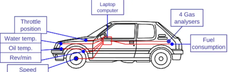
Ariztegui (2004). A scheme of on-board instrumentation is shown in Figure 1.
The second vehicle used is a diesel passenger car, Peugeot 406 BK STDT 2.1, with a direct injection turbo
engine, 2088 cm3 and 1485 kg. It has been instrumented with a non-intrusive universal on-board emission
measurement system (MIVECO-PEMS) and a portable global activity measurement system (PGAMS), both developed as part of research project for real life emission measurement. The block diagram of the MIVECO PGAMS/PEMS and the scheme of MIVECO PEMS are shown in Figure 2.
The electronic prototype PGAMS (Portable Global Activity Measurement System) aims to record, simultaneously and synchronously, the activity of the main agents involved on car pollutant emissions: driver, vehicle and route. Its hardware architecture is based on three subsystems: sensorial, conditioning and acquisition, processing and monitoring (local and remote). The PGAMS is a system that can be boarded on any type of vehicle.
The MIVECO on-board emission measurement system (MIVECO-PEMS) for Diesel/petrol HD and LD vehicles, depicted in Figure 3, is based on fast response commercial analysers and a self designed exhaust flow meter. The
MIVECO-PEMS are conformed by a NDIR analyzer for CO2 and CO, a non-sampling Zirconia type NOX -O2
analyzer, a FID for unburned hydrocarbons (HC), and a Lambda Meter. The signals generated by each analyzer are collected by an acquisition system that uses Labview® software at 10 Hz data recording frequency. The flow meter consists of a Pitot tube for gases with high moisture content, which prevents that condensation may block pressure ducts and a differential pressure gauge of high sensitivity and response rate, capable of detecting pressure changes at a frequency up to 1kHz. This makes it possible to detect the pulses of flow that occur in the engine at idle.
Figure 1: Scheme of on-board instrumentation in the petrol car.
Fuel consumption
Laptop computer
Throttle position
Water temp.
Oil temp. Rev/min
Speed
4 Gas analysers
Fuel consumption
Laptop computer
Throttle position
Water temp.
Oil temp. Rev/min
Speed
Environment & Transport / Environnement & Transports SECTOR 3 SECTOR 4 SECTOR 5 SECTOR 7 SECTOR 6 SECTOR 3 SECTOR 4 SECTOR 5 SECTOR 7 SECTOR 6 SECTOR 3 SECTOR 4 SECTOR 5 SECTOR 7 SECTOR 6
Figure 2: On-board instrumentation in the diesel car a) Block diagram of the MIVECO PGAM/PEMS. b) Scheme of the MIVECO PEMS (portable emission measurement system).
Figure 3: MIVECO-PEM System arrangement in the diesel car.
Urban circuit
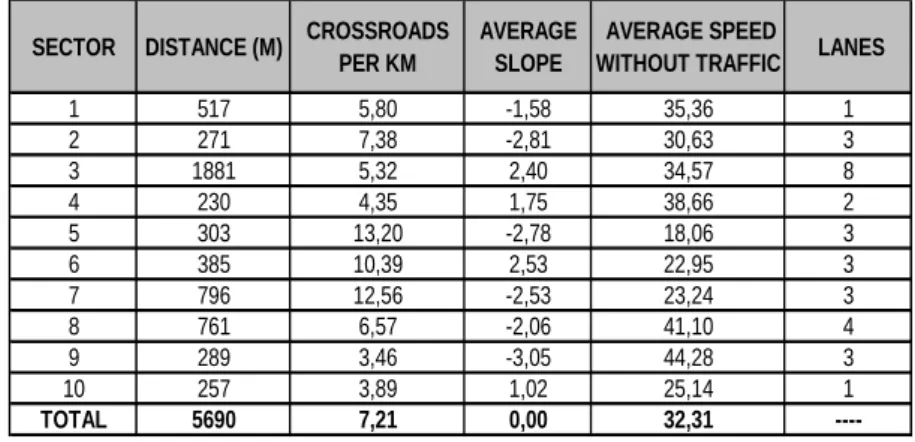
The measures were carried out in a specific urban circuit in Madrid City, called “Madrid-UPM Circuit”, which include most of the types of streets there are downtown, like local, secondary, principal and arterial. To know the influence of the type of street, the whole route was divided into 10 sectors, as shown in Figure 4 and whose characteristics are presented. 50 journeys were realized by this route, 40 of them with the petrol passenger car and
the others with the diesel passenger car. A portion of the petrol car journeys were made in days off, in order to
obtain experimental data about average speed without traffic, which were used as a baseline. Remaining trips were made in normal traffic conditions.
Figure 4: Madrid-UPM Circuit and table of characteristics per sector.
SECTOR DISTANCE (M) CROSSROADS PER KM
AVERAGE SLOPE
AVERAGE SPEED
WITHOUT TRAFFIC LANES
1 517 5,80 -1,58 35,36 1
2 271 7,38 -2,81 30,63 3
3 1881 5,32 2,40 34,57 8
4 230 4,35 1,75 38,66 2
5 303 13,20 -2,78 18,06 3
6 385 10,39 2,53 22,95 3
7 796 12,56 -2,53 23,24 3
8 761 6,57 -2,06 41,10 4
Flow meter MIVECO
Lambda meter
ETASLA4
NOXy O2 analyzer
HORIBA MEXA 720
HC analyzer ThermoFID PT EXHAUST GASES CO CO2 N2 N2 CO Analyzer SIGNAL 9000 s a m pl ing t u be heated line Air cooler Calibration gases Cold line Signal line Pitot tube Filter T Differential Pressure Sensor Δ p On-board equipments N2 N2 CO2 N2 N2 N2 N2 N2 H2 Flow meter MIVECO Lambda meter ETASLA4
NOXy O2 analyzer
HORIBA MEXA 720
HC analyzer ThermoFID PT EXHAUST GASES CO CO2 N2 N2 CONN22 CO Analyzer SIGNAL 9000 s a m pl ing t u be heated line Air cooler Calibration gases Cold line Signal line Pitot tube Filter TT Differential Pressure Sensor Δ p On-board equipments N2 N2 CONN222
CO2
N2
N2 NNN222 N2
N2
N2 HNN222 H2 Processing and Monitoring System Sensorial Remote Supervision Acquisition System PEM Gases Partícles EMC PAM Motor Route Driver GSM USB RS232
variables were calculated –for each sector and for the entire route-, based on the results of several researches carried out by Ericsson (2000, 2001 and 2006): average speed (km/h), average running speed (km/h) – average
speed excluding idle time, average acceleration (m/s2), average deceleration (m/s2), percentage of time spent in
different operating modes (gear) or idle, like percentage of time on high gears (3rd, 4th and 5th), percentage of
time over 2000 min-1, average value of the product of Instantaneous speed and acceleration, called “demand of
acceleration” as defined by Ericsson (2001), stop time per crossroad.
Driving STYLE, Street and Traffic variables
Because of driving style have a great influence over driving patterns, three kinds of driving styles have been compared as defined by De Vlieger (1997-2000), Ericsson (2000-2001) and Takada (2007): calm driving -where the driver anticipates movements avoiding sudden accelerations-, normal driving -where accelerations and decelerations are moderated- and aggressive driving, -where violent or sudden acceleration and heavy braking are present-. The calm driving corresponds with the concept of “Eco-driving style”, described above.
In addition to the fact that the driving style strongly affects the specific driving pattern, many research works -Brundell-Freij and Ericsson (2005), Ericsson (2001), Ericsson (2000), Rosqvist (2003), De Vlieger (2000) and Ericsson (2006)- have showed that road infrastructure and traffic density have great influence too. So, in this study a Street-Index and a Traffic-Index have been defined in order to measure the degree of constriction that those aspects impose on the way to any driver to make a particular trip.
The variables included in the Street-Index are: type of road, slope and density of crossroads. The type of road is an index defined from 0 to 1 that indicates the traffic constriction as follow: 0 for very high constriction and 1 for very low constriction. In this order, 0.15 for local street, 0.30 for secondary, 0.45 for main, 0.6 for arterial, 0.75 for bypass street and 0.9 for highway. The Street-Index was based on a statistical study conducted with the experimental data obtained with the petrol car during day off journeys, following that average speed without traffic can be expressed in terms of those static variables as follows:
Average_speed_without_traffic = 34,25 – 0,90*slope + 32,28*Type_of_street – 2,15 * crossroads/km
(R-squared: 83,4%, indicated that this model explains 83,4% of the variability in Average_speed_without_trafic. And, since P-value in the ANOVA table is less than 0.01, there is a statistically significant relationship between the variables at the 99% confidence level)
To obtain a normal Street-Index –from 0 for low constriction and 1 for high constriction-, was necessary to apply the following equation:
Street-Index = Si =1,25 - 0,025 * Average_speed_without_traffic
In order to determinate the Traffic-index, two associated variables that are naturally related with traffic flow were studied: stop time per crossroad and average speed per average speed without traffic. The Figure 5 shows the relationship between these variables.
Since there has been statistically demonstrated that neither average_speed nor these two variables have any correlation with the specific driving style (maximum R_Squared=5%, indicating that the driving style explains maximum 5% of the variability in Average_speed and in these traffic variables), and Average_speed_without_traffic depends only on road infrastructure, the Traffic-Index has been defined proportionally to the Average speed per average speed without traffic, with a numerical value from 0 to 1 indicating very low and very high traffic density
respectively, as shown bellow:
Traffic_index = Ti = 1 – 0.67*Average_speed_per_average_speed_without_traffic
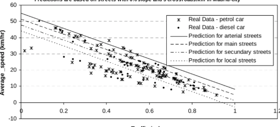
This makes it possible to obtain an equation to predict the average speed for a given route based on the street-index and traffic-street-index, as shown in the next equation and in the Figure 6 obtained for different street types:
Environment & Transport / Environnement & Transports
Figure 5: Traffic variables relationship.
Based on petrol passenger car EURO1 experimental data in real urban traff ic in Madrid city
-20 0 20 40 60 80 100
0 0.2 0.4 0.6 0.8 1 1.2 1.4 1.6
Average_speed_per_average_speed_without_traffic
Sto
p
ti
m
e
pe
r c
ro
s
s
roa
d
(s
)
low traffic density high traffic density
Figure 6: Variation of average speed with traffic index for different streets.
Predictions are based on streets w ith 0% slope and 5 crossroads/km in Madrid-city
-10 0 10 20 30 40 50 60
0 0.2 0.4 0.6 0.8 1 1.2
Traffic-index
A
ver
ag
e _sp
eed
(km
/h
r)
Real Data - petrol car Real Data - diesel car Prediction for arterial streets Prediction for main streets Prediction for secundary streets Prediction for local streets
2 – Results
The only linearly independent variables related to driving style are average acceleration and percentage of time
over 2000 min-1. This has enabled to define the Dynamic_Performance_Index that allows assessing the driving
style, as shown below:
Dynamic_Performance_Index = DPI = -0,17 + 0,55 * Average_acceleration + 0.006 * %_time_>2000rpm
(R-squared = 70%, P-value=0.00)
The definition of the Dynamic_Performance_index lets to predict the value of the most important dynamic variables based only on the characteristics of the road infrastructure (Street_index - Si), traffic density (traffic_index - Ti) and driving style (Dynamic_Performance_index-DPi) as shown in the following equations:
Average_acceleration = 0,05 + 0,29 * Si + 0.34 * Ti + 1,13 * DPi (R-squared = 83%, P-value=0.00)
% time>2000 rpm = 23,33 - 26,34 * Si – 31,27 * Ti + 61,39 * DPi (R-squared = 75%, P-value=0.00)
% time on large gear = 123,99 - 61,46 *Si – 95,94* Ti - 29,45* DPi (R-squared = 55%, P-value=0.00)
Demand of acceleration = 25,54 - 11,75 * Si – 22,43* Ti + 25,48* DPi (R-squared = 82%, P-value=0.00).
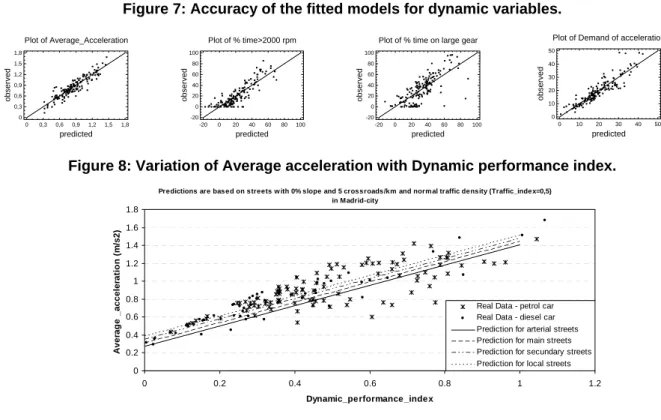
The accuracy of the fitted models for these variables is shown graphically in Figure 7. Additionally, the prediction of the average acceleration, for different types of streets, is shown in Figure 8.
Plot of Average_Acceleration
predicted
observed
0 0,3 0,6 0,9 1,2 1,5 1,8 0 0,3 0,6 0,9 1,2 1,5 1,8
Plot of % time>2000 rpm
predicted
observed
-20 0 20 40 60 80 100 -20 0 20 40 60 80 100
Plot of % time on large gear
predicted
observed
-20 0 20 40 60 80 100 -20 0 20 40 60 80 100
Plot of Demand of acceleration
predicted
observed
0 10 20 30 40 50
0 10 20 30 40 50
Figure 8: Variation of Average acceleration with Dynamic performance index.
Predictions are based on streets w ith 0% slope and 5 crossroads/km and norm al traffic density (Traffic_index=0,5) in Madrid-city 0 0.2 0.4 0.6 0.8 1 1.2 1.4 1.6 1.8
0 0.2 0.4 0.6 0.8 1 1.2
Dynamic_performance_index A ver a g e _a ccel e rat io n ( m /s 2)
Real Data - petrol car Real Data - diesel car Prediction for arterial streets Prediction for main streets Prediction for secundary streets Prediction for local streets
Petrol Passenger car Emission factors
To investigate the linear relationship between emission factors and each of the variables considered, analysis of variance was carried out using Pearson coefficient. The Table 1 presents a summary of the main variables (for better visualization only are shown correlation coefficient greater than 0.2, although correlation is considered significant when the coefficient is greater than 0.3).
Table 1: Pearson Correlation coefficients for emission factors
FE HC FE CO FE CO2 FE NOX
Driving
behaviour Driver perception 0.24 0.49
Dynamic_performance 0.23 0.45
Street 0.20
Traffic 0.40 0.41 0.45
Average acceleration 0.25 0.28 0.52 0.47
Average desaceleration -0.22 -0.36 -0.34
% time on large gear -0.30 -0.31 -0.58
% time>2000 rpm -0.25 -0.29 0.25
Demand of acceleration 0.30
Average speed (km/hr) -0.37 -0.39 -0.58
Stop time / crossroad 0.31 0.29 0.59
Average speed / Average
speed without traffic -0.37 -0.40 -0.41
Type_of_street -0.22
Slope Crossroads/km
FE HC - 0.89 0.44
FE CO 0.89 - 0.40
FE CO2 0.44 0.40 - 0.34
FE Nox 0.34
-Dynamic variables EMISSION FACTORS (g/km) Traffic variables Road infrastructure
BASED ON REAL TIME MEASUREMENT WITH A PETROL TOURING CAR (EURO1) IN URBAN TRAFFIC IN MADRID CITY
EMISSION FACTORS (g/km)
Index
The table of Pearson correlation coefficients –Table2-, confirms that the petrol car fuel consumption (CO2
emission) increases with average acceleration, stop time per crossroad and decreases with average speed and the
use of high gears. Additionally, it is noted that the NOX emission is primarily associated to the acceleration and
hence to the driving style. This is an expected result due to the fact that stronger accelerations are related to higher
cylinder gas temperatures, which favours NOX formation. Furthermore, the emissions of HC and CO, closely
related to each other, are affected by traffic density, although the correlation is weaker.
To quantify the influence of traffic, street infrastructure and driving style over emissions and fuel consumption,
multiple linear regression analysis was performed. It has been found that only CO2 emissions are directly related
Environment & Transport / Environnement & Transports
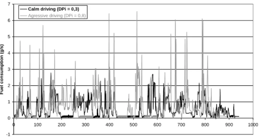
Influence study of driving behaviour in real traffic in Madrid city INSTANTANEOUS FUEL CONSUMPTION
2 3 4 5 6 7 Fu el co nsum p tio n (g /s )
Calm driving (DPi = 0,3)
Agressive driving (DPi = 0,8)
EF_CO2 = -31,57 + 131,89 * Si + 127,94 * DPi + 220,26 * Ti (R-squared = 48%, P-value=0.00)
EF_CO = 0,76 + 3,90 * Ti (R-squared = 17%, P-value=0.00)
EF_HC = 0,04 + 0,18 * Ti (R-squared = 16%, P-value=0.00)
EF_ NOX = -0,02 + 0,14 * DPi (R-squared = 21%, P-value=0.00)
The model generated for CO2 emission factor (fuel consumption) explains nearly 50% of its variability, while
only explained 16%, 17% and 21% of the variability of the factors CO, HC and NOX respectively. However to
illustrate the trends found, the Figure 10 shows the prediction of the CO2 emission factor (fuel consumption) with
respect to driver style, for different types of streets and traffic conditions.
Figure 9: Accuracy of the fitted models for emission factors.
Plot of Fitted Model for CO emission factor
Traffic_index
FE_CO (g/
k
m)
0 0,3 0,6 0,9 1,2 0 2 4 6 8 10
Plot of Fitted Model for HC emission factor
Traffic_index
FE_HC (g/km)
-0,3 0 0,3 0,6 0,9 1,2 0 0,1 0,2 0,3 0,4 0,5
Plot of Fitted Model for NOx emission factor
Dynamic_performance_index
FE_NOx (g/km)
0 0,2 0,4 0,6 0,8 1 0
0,1 0,2 0,3 0,4
Plot of CO2 Emission Factor (g)km)
predicted
observed
0 100 200 300 400 500 0 100 200 300 400 500
Figure 10: CO2 Emission Factor & Dynamic performance index.
Predictions are based on streets with 0% slope and 5 crossroads/km in Madrid-city
0 50 100 150 200 250 300 350 400
0 0.1 0.2 0.3 0.4 0.5 0.6 0.7 0.8 0.9 1
Dynamic_performance_index C O 2 E m issi o n F act o r ( g /km ) Real Data Arterial streets Main streets Secundary streets Local streets Normal traffic; Ti=0.5
Heavy traffic; Ti=0.8
Petrol Passenger car Emission factors
The Figure 11 illustrates the comparative curve for instantaneous consumption and average emission factors for two different driving styles. It is noted that in addition to the peaks of consumption are higher in aggressive driving, emission factors are also.
Figure 11: Instantaneous fuel consumption and total emission factor for diesel car in different driving style.
Influence study of driving behaviour in real traffic in Madrid city
EMISSION FACTORS (EF)
0 0,1 0,2 0,3 0,4 0,5 0,6
EF CO EF HC EF NOx
g/
k
m
Calm driving (DPi=0,3) Agressive driving (DPi=0,8)
Influence study of driving behaviour in real traffic
in Madrid city CO2 EMISSION FACTORS (EF)
Average speed in day off trips with “normal” driving, depends only on the street configuration, and is useful to independently evaluate the effect of the street characteristics over the driving style. It is the best parameter to define the Street Index.
In spite of the fact that the Traffic Index has been defined only as a function of the average speed to day off average speed ratio, for future research the spot time per crossroad should be included, because it has a significant influence on fuel consumption.
Traffic density has almost double weight that aggressiveness and street constrictions on CO2 emissions, it
confirms that congestion and traffic flow is a relevant factor to be controlled to reduce these emissions in a big town as Madrid Town.
In the case of the petrol car, CO and HC emissions are correlated, as shown in table 1. It is due to the fact that both pollutants are coming from combustion problems with rich mixtures. The fact that no correlations could be found between these pollutants and vehicle dynamic variables, are probably due to the fact that there are some moments in which the injection system cannot control the air fuel ratio dealing to transitory rich mixtures when the gas pedal is released. But probably with a more advanced injection system, this situation will not appear.
Although correlation between NOX emissions and DPi obtained in this work is lean, it is actually a correlation
that should be previously expected because of higher engine loads when aggressiveness is higher. Then more
tests in different types of car are needed to understand better the relationship between NOX emissions and real
traffic situations.
The graphics of instantaneous emissions in the diesel car tests show a significant influence of driving style on pollutant emissions and fuel consumption, as should be expected. More tests are needed obtain more statistically consistent results.
Acknowledgments
The authors would like to acknowledge the financial backing for this project provided by the Ministry of Environment and Rural and Marine Affairs of Spain. The authors also wish to acknowledge the contributions of Emilio Cano by the preliminary treatment of the experimental data and to David Nieto, Diego Perez and Alfredo Gonzalez for mounting equipment in vehicles and carrying out of tests.
References
Ariztegui J., J. Casanova & M. Valdes (2004): A structured methodology to calculate traffic emissions inventories for city centres. Science of the Total Environment. Volume 334-335. (2004) p 101-109.
Brundell-Freij K. & Ericsson E. (2005): Influence of street characteristics, driver category and car performance on urban driving patterns. Transportation Research Part D: Transport and Environment. Volume 10, Issue 3, May 2005, p 213-229.
Casanova J., M. Valdes & J. Ariztegui (2001): The influence of car fleet composition on urban pollutant emissions. Application to the City of Madrid. Proceedings of 10th International Symposium "Transport and Air Pollution". September 17-19, 2001 -- Boulder, Colorado USA.
Casanova J., J. Ariztegui & M. Valdes (2004): Comparative study of two different on-board emission measurement systems. Proceedings of the Word Automotive Congress, FISITA 2004. Barcelona, Spain 2004.
Ref:F2004V053.
Casanova J., S. Margenat & J. Ariztegui (2005): Impact of driving style on Pollutant Emissions and Fuel
Consumption for Urban Cars. Proceedings of the 1st International Congress of Energy and Enviroment
Engineering and Management. Portalegre, Portugal. 2005. p175
De Vlieger I. (1997): On board emission and fuel consumption measurement campaign on petrol-driven passenger cars. Atmospheric Environment. Volume 31, Issue 22, November 1997, p 3753-3761.
De Vlieger I., D. De Keukeleere & J. G. Kretzschmar (2000): Environmental effects of driving behaviour and congestion related to passenger cars. Atmospheric Environment. Volume 34, Issue 27, 2000, Pages 4649-4655.
Environment & Transport / Environnement & Transports
Ericsson E. (2001): Independent driving pattern factors and their influence on fuel-use exhaust emission factors. Transportation Research Part D: Transport and Environment. Volume 6, Issue 5, September 2001, p 325-345.
Ericsson E., H. Larsson & K. Brundell-Freij (2006): Optimizing route choice for lowest fuel consumption – Potential effects of a new driver support tool. Transportation Research Part C. Volume 14 p369.
Gao Y. & M.D. Checkel (2007): Experimental Measurement of On-Road CO2 Emission & Fuel Consumption
Functions. SAE paper 2007-01-1610.
Johansson H., P. Gustafsson, M. Henke & M. Rosengren (2003): Impact of EcoDriving on emissions. Proceedings
of the 12th International Symposium Transport and Air Pollution. No. 92. Vol I, p113.
Miyazaki T., Y. Takada & N. Lida (2002): Development of On-Board System to Measure Running Condition and
Actual NOX Emissions From Freight Vehicle. SAE paper 2002-01-0613.
Ntziachristos L. & Z. Samaras (2000): Copert III. Computer programme to calculate emissions from road transport. European Environment Agency 2000; 53-54:61-5.
Pelkmans L. & P. Debal (2006): Comparison of on-road emissions with emissions measured on chassis dynamometer test cycles. Transportation Research Part D: Transport and Environment. Volume 11, Issue 4, July 2006, p 233-241.