Evolution in HPC Environments
Diego Darriba L ´
opez
Departmento de Electr´onica e Sistemas
Universidade da Coru˜
na
Departmento de Bioqu´ımica, Xen´etica e Inmunolox´ıa
Universidade de Vigo
PhD Thesis
Selection of Models of Genomic Evolution in
High Performance Computing Environments
Diego Darriba L´opez
October 2015
PhD Advisors:
Dpto. de Electr´onica y Sistemas Universidade da Coru˜na
Dpto. de Electr´onica y Sistemas Universidade da Coru˜na
Dr. David Posada Gonz´alez Catedr´atico de Universidad
Dpto. de Bioqu´ımica, Gen´etica e Inmunolog´ıa Universidade de Vigo
CERTIFICAN
Que la memoria titulada “Selection of Models of Genomic Evolution in HPC Envi-ronments” ha sido realizada por D. Diego Darriba L´opez bajo nuestra direcci´on en el Departamento de Electr´onica y Sistemas de la Universidad de A Coru˜na y en el Departamento de Bioqu´ımica, Gen´etica e Inmunolog´ıa de la Universidade de Vigo en r´egimen de cotutela, concluye la tesis doctoral que presenta para optar al grado de Doctor en Ingenier´ıa Inform´atica con la Menci´on de Doctorado Internacional.
En A Coru˜na y Vigo, a 20 de Octubre de 2015
Fdo.:
Guillermo L´opez Taboada Director de la Tesis Doctoral
Fdo.:
Ram´on Doallo Biempica Director de la Tesis Doctoral
Fdo.:
David Posada Gonz´alez Director de la Tesis Doctoral
This research project would not have been possible without the support of many people. I wish to express my gratitude to my PhD advisors, Guillermo, Ram´on and David who were abundantly helpful and offered invaluable assistance, support and dedicated guidance.
Special thanks also to all my collaborators and fellow group members; Adri´an, Andi´on, Andr´es, CH, Dyer, Iv´an, Jorge, Jurjo, Mois´es, Porta, Raquel, Rober, Sabela and To˜no from GAC; ´Alex, Andr´es, Carlos, Diego, Klaus, Leo, Mar´ıa, Mateus, Merchi, Miguel A., Miguel F., Ram´on and Sara from XB5/Phylogenomics; Alexey, Andre, Fernando, Jiajie, Kassian, Nikos, Paschalia, Pavlos, Solon and Tomas from H-ITS. Thank you all for being so collaborative and helpful. I would like to thank my parents, brothers and family for their unconditional support, as well as my friends from Lugo, A Coru˜na and Heidelberg, who have always stood by me.
I would like to sincerely thank Prof. Dr. Alexandros Stamatakis and the Scientific Computing Group for hosting me during my three-month research visit to the Heidelberg Institute for Theoretical Studies (Germany). Moreover, I am grateful to CESGA (Galicia Supercomputing Center) for providing access to the clusters and supercomputers that have been used as testbeds for this work.
mechanism as a black box.
A introducci´on das tecnolox´ıas de sequenciaci´on de nova xeraci´on, ou “Next-Generation Sequencing” (NGS), representou un notable cambio no campo da filo-xen´etica. A cantidade de informaci´on molecular dispo˜nible est´a a crecer cada vez m´ais r´apido, propiciando o desenvolvemento de m´etodos e ferramentas de an´alise m´ais eficientes, as´ı coma o uso de t´ecnicas de computaci´on de altas prestaci´ons (HPC) para acelerar as an´alises. O campo est´a a cambiar velozmente da an´alise filoxen´etica (i.e., estudo dun ou un conxunto reducido de xens) ´a filoxen´omica (i,e., estudo de centos ou millares de xens de xenomas completos ou incompletos). Moi-tos m´etodos filoxen´eticos requiren o uso de modelos probabil´ısticos de evoluci´on molecular, e ´e co˜necido que o uso dun modelo ou outro pode derivar en diferentes estimaci´ons filoxen´eticas. Tanto modelos sub- como sobreparametrizados presen-tan desvantaxes en termos de precisi´on. Polo presen-tanto, existen ferramentas populares que fan uso de marcos estad´ısticos para seleccionar o modelo que mellor se axus-ta aos datos, buscando o mellor compromiso entre likelihood (verosimilitude) e parametrizaci´on.
Esta tese doutoral presenta o dese˜no, implementaci´on e evaluaci´on de m´eto-dos HPC para seleccionar o modelo de evoluci´on m´ais adecuado, en conxunto co desenvolvemento de novas funci´ons orientadas a facer m´ais sinxela a an´alise de datos filoxen´eticos. En particular, extendemos e paralizamos as d´uas ferramentas m´ais populares para a selecci´on de modelos de ADN e prote´ınas, jModelTest e ProtTest. Adem´ais, esta tese presenta o dese˜no, implementaci´on e evaluaci´on de algoritmos para a an´alise r´apida e precisa de datos xen´omicos. Creamos unha ferra-menta incorporando todas estas t´ecnicas, denominada PartitionTest, delegando a computaci´on principal na librer´ıa de an´alise filoxen´etica PLL. Finalmente, fixemos un estudo de simulaci´ons sobre a importancia do uso de t´ecnicas de selecci´on de modelos en datos xen´omicos, e o seu impacto na precisi´on ao recuperar os modelos
La introducci´on de las tecnolog´ıas de secuenciaci´on de nueva generaci´on, o “Next-Generation Sequencing” (NGS), ha representado un notable cambio en el campo de la filogen´etica. La cantidad de informaci´on molecular disponible est´a cre-ciendo cada vez m´as r´apido, propiciando el desarrollo de m´etodos y herramientas de an´alisis m´as eficientes, as´ı como el uso de t´ecnicas de computaci´on de altas prestaciones (HPC) para acelerar los an´alisis. El campo est´a cambiando r´apida-mente del an´alisis filogen´etico (i.e., estudio de uno o un conjunto reducido de genes) al filogen´omico (i,e., estudio de cientos o miles de genes de genomas com-pletos o incomcom-pletos). Muchos m´etodos filogen´eticos requieren utilizar modelos probabil´ısticos de evoluci´on molecular, y es sabido que el uso de un modelo u otro puede derivar en diferentes estimaciones filogen´eticas. Tanto modelos sub- como sobreparametrizados presentan desventajas en t´erminos de precisi´on. Por lo tanto, existen herramientas populares que hacen uso de marcos estad´ısticos para selec-cionar el modelo que mejor se ajuste a los datos, buscando el mejor compromiso entre likelihood (verosimilitud) y parametrizaci´on.
Esta tesis doctoral presenta el dise˜no, implementaci´on y evaluaci´on de m´eto-dos HPC para seleccionar el modelo de evoluci´on m´as adecuado, conjuntamente con el desarrollo de nuevas funciones orientadas a facilitar el an´alisis de datos fi-logen´eticos. En concreto, hemos extendido y paralizado las dos herramientas m´as populares para selecci´on de modelos de ADN y prote´ınas, jModelTest y ProtTest. Adem´as, esta tesis presenta el dise˜no, implementaci´on y evaluaci´on de algoritmos para el an´alisis r´apido y preciso de datos gen´omicos. Hemos creado una herra-mienta incorporando todas estas t´ecnicas, denominada PartitionTest, delegando la computaci´on principal en la librer´ıa de an´alisis filogen´etico PLL. Finalmente, hemos hecho un estudio de simulaciones sobre la importancia del uso de t´ecnicas de selecci´on de modelos en datos gen´omicos, y su impacto en la precisi´on al recuperar
The irruption of Next-Generation Sequencing (NGS) technologies has changed dramatically the landscape of phylogenetics. The available molecular data keeps growing faster and faster, prompting the development of more efficient analytical methods and tools, as well as the use of High Performance Computing (HPC) techniques for speeding-up the analyses. The field is rapidly changing from phy-logenetics (i.e., the study of a single or a few genes) to phylogenomics (i.e., the study of hundreds or thousands of genes from incomplete or complete genomes). Many phylogenetic methods require the use of probabilistic models of molecular evolution, and it is well known that the use of different models may lead to dif-ferent phylogenetic estimates. Both under- and overparameterized models present disadvantages in terms of accuracy. Therefore, there are popular tools that employ statistical frameworks for selecting the most suitable model of evolution for the data, finding the best trade-off among likelihood and parameterization.
This PhD thesis presents the design, implementation and evaluation of HPC methods for selecting the best-fit model of evolution, together with improved fea-tures that facilitate the analysis of single-gene data. In particular, we extended and parallelized the two most popular tools for selecting the best-fit model of evolution for DNA and proteins, jModelTest and ProtTest. Furthermore, this the-sis presents the design, implementation and evaluation of algorithms for fast and accurate analysis of multi-gene data. We created a tool incorporating all these techniques, called PartitionTest, delegating the core computations to the Phylo-genetic Likelihood Library (PLL). Finally, we made a simulation study on the importance of using model selection techniques on multi-gene data, and its impact on the accuracy retrieving the true generating models and, most important, the
Preface 1
1. Introduction 7
1.1. Phylogenetic Inference . . . 7
1.1.1. Models of Evolution . . . 8
1.1.2. Phylogenetic Trees . . . 13
1.1.3. Computing the Likelihood of a Tree . . . 15
1.1.4. Selecting the Best-Fit Model of Evolution For Single-Gene Alignments . . . 21
1.1.5. Selecting the Best-Fit Model of Evolution For Multigene Alignments: Partitioning . . . 27
1.2. Software for Model Selection . . . 31
1.2.1. ProtTest 2.x . . . 31
1.2.2. ModelTest and jModelTest 1.x . . . 32
1.3. Scope and Motivation . . . 34
1.4. Main Objectives of the Thesis . . . 34
2. ProtTest 3 - Protein Model Selection 37
3. HPC Model Selection for Multicore Clusters 45
4. DNA Model Selection on the Cloud 61
5. jModelTest2 - Nature Methods 69
6. PartitionTest - Multigene Model Selection 85
7. Discussion 113
8. Conclusions 117
9. Future Work 119
10.A Summary in Spanish 121
10.1. Introducci´on . . . 121
10.2. Organizaci´on de la Tesis . . . 123
10.3. Medios . . . 125
10.4. Discusi´on . . . 127
10.5. Conclusiones . . . 130
10.6. Trabajo Futuro . . . 132
10.7. Principales Contribuciones . . . 133
1.1. Standard amino-acid abbreviations . . . 8
1.2. Substitution models available in jModelTest. . . 33
1.1. Graphic representation of a rooted tree for 3 species. . . 14
1.2. Graphic representation of an unrooted tree for 4 species (in the middle). A root can be placed on any of the 5 branches, producing 5 different rooted topologies out of the same unrooted topology. . . 15
1.3. Conditional likelihood vectore entries are computed based on the CLVs of the children nodes, the model and the transition probability matrices P(bqp) andP(brp). . . 18
1.4. Probability density function of the Γ distribution . . . 21
1.5. Example of a forward hierarchy of Likelihood Ratio Tests (hLRT) for 6 candidate models . . . 24
1.6. Example of dynamical Likelihood Ratio Tests (dLRT) . . . 24
1.7. Partitioning schemes for N = 4. Numbers and colors represent the different partitions. In this example, there are 2N−1 = 15 partitions and B(N) = 15 partitioning schemes. . . 30
4.1. jModelTest.org login screen . . . 65
4.2. jModelTest.org MSA input . . . 65
4.3. jModelTest.org execution options . . . 66
4.4. jModelTest.org running status . . . 67
Work Methodology
This thesis follows a classical approach in scientific and technological research: analysis, design, implementation and evaluation. Thus, the thesis starts with the analysis of the importance of selecting the best-fit models of evolution, the options already available and the feasibility and impact analysis of providing High Perfor-mance Computing capabilities to this task. We first tackled the model selection for single-gene DNA and protein data, re-designing from scratch the two most popular tools, adding HPC and fault tolerance capabilities, as well as new meth-ods and algorithms. We then evaluated the accuracy and performance in several representative architectures.
Next, we analysed the problem of model assignment for multigene data, a prob-lem also known aspartitioning. Among available options for Maximum-Likelihood parameter estimation and phylogenetic searches, the use of the Phylogenetic Likeli-hood Library (PLL) turned out to be the most flexible approach. We collaborated in the development of PLL, adding flexibility for managing partitions of data (i.e., subsets of the data where different models can be used), from which we devised and implemented heuristic algorithms in linear and polynomial time for select-ing the best-fit partitionselect-ing scheme. Finally, we evaluated the partitionselect-ing and phylogenetic accuracy of our algorithms using simulated and real-world data sets.
Structure of the Thesis
In accordance with the current regulations of the University of A Coru˜na, this PhD dissertation has been structured as a compilation thesis (i.e., merging research articles). In particular, this thesis comprises three JCR-indexed journal scientific articles, presented in chapters 3, 4 and 5, together with two additional articles of great interest within the scope of the work. The thesis begins with the Introduction chapter, intended to give the reader a general overview of model selection in phylogenetics.
This chapter introduces the scope, main motivations and objectives of the thesis.
The scientific articles included in the compilation, each one presented as a separate chapter (Chapters 2-6) are the following:
Chapter 2: Darriba, D., Taboada, G. L., Doallo, R., & Posada, D. (2011). ProtTest 3: fast selection of best-fit models of protein evolution. Bioinfor-matics, 27(8), 1164-1165.
Impact factor: 4.981,547 citations as of October 2015.
Chapter 3: Darriba, D., Taboada, G. L., Doallo, R., & Posada, D. (2013). High-performance computing selection of models of DNA substitution for multicore clusters. International Journal of High Performance Computing Applications, 1094342013495095.
Impact factor: 1.477,4 citations as of October 2015.
Chapter 4: Santorum, J. M., Darriba, D., Taboada, G. L., & Posada, D. (2014). jmodeltest.org: selection of nucleotide substitution models on the cloud. Bioinformatics, btu032.
Impact factor: 4.981
Chapter 5: Darriba, D., Taboada, G. L., Doallo, R., & Posada, D. (2012). jModelTest 2: more models, new heuristics and parallel computing. Nature methods, 9(8), 772-772.
Chapter 6: Darriba, D., & Posada, D. (2015). The impact of partitioning on phylogenomic accuracy. bioRxiv, 023978.
In Chapter 7 we include a general discussion of the included research articles. Chapter 8 describes the conclusions of the thesis. Finally, in Chapter 9 we describe the future work.
Funding and Technical Means
Working material, human and financial support primarily by the Computer Architecture Group of the University of A Coru˜na and the Phylogenomics Group of the University of Vigo.
Access to bibliographical material through the libraries of the Universities of A Coru˜na and Vigo.
Additional funding through the following research projects:
• Regional funding by the Galician Government (Xunta de Galicia) under the Consolidation Program of Competitive Research Groups (Computer Architecture Group, refs. GRC2013/055 and 2010/6), Galician Network of High Performance Computing (ref. 2010/53), and Galician Network of Bioinformatics (ref. 2010/90).
• European Research Council (Phylogenomics Group, ref. ERC-2007-Stg 203161-PHYGENOM).
• The Ministry of Science and Innovation of Spain under Project TIN2010-16735 (Computer Architecture Group).
• Amazon Web Services (AWS) research grant “EC2 in phylogenomics”.
• The Spanish Ministry of Science and Education under project BFU2009-08611 (Phylogenomics Group)
• Pluton cluster (Computer Architecture Group, University of A Coru˜na, Spain). Initially, 16 nodes with 2 Intel Xeon quad-core Nehalem-EP processors and up to 16 GB of memory, all nodes interconnected via InfiniBand DDR and 2 of them via 10 Gigabit Ethernet. Additionally, two nodes with one Intel Xeon quad-core Sandy Bridge-EP processor and 32 GB of memory, interconnected via InfiniBand FDR, RoCE and iWARP, and four nodes with one Intel Xeon hexa-core Westmere-EP processor, 12 GB of memory and 2 GPUs NVIDIA Tesla “Fermi” 2050 per node, interconnected via InfiniBand QDR. Later, 16 nodes have been added, each of them with 2 Intel Xeon octa-core Sandy Bridge-EP processors, 64 GB of memory and 2 GPUs NVIDIA Tesla “Kepler” K20m per node, interconnected via InfiniBand FDR.
• Diploid cluster (Phylogenomics Group, University of Vigo, Spain). (1) One fat node with 4 Intel Xeon ten-core Westmere-EX processors and 512 GB of memory, (2) 30 nodes with 2 Intel Xeon E5-420 quad-core Harpertown processors (a total of 8 cores) and 16 GB of memory, and (3) 44 nodes with 2 Intel Xeon X5675 hexa-core Westmere-EP (a total of 12 cores); 50 GB of memory and Hyperthreading disabled.
• Magny cluster(Heidelberg Institute for Theoretical Studies, Heidelberg, Germany). (1) 2 Sandy Bridge nodes with 2 Intel Xeon E5-2630 hexa-core Sandy Bridge processors (a total of 12 hexa-cores) and Hyperthreading disabled;32 GB of memory, and (2) Magny-Cours node with 4 AMD Opteron 6174 12-core processors (a total of 48 cores); 128 GB of mem-ory.
• Finis Terrae supercomputer (Galicia Supercomputing Center, CESGA,
Spain): 144 nodes with 8 Intel Itanium-2 dual-core Montvale proces-sors and 128 GB of memory, interconnected via InfiniBand DDR. Ad-ditionally, we have used one Superdome system with 64 Intel Itanium-2 dual-core Montvale processors and 1 TB of memory.
60.5 GB of memory and 4 local storage disks per instance; (3) CG1, 2 Intel Xeon quad-core Nehalem-EP processors, 22 GB of memory, 2 GPUs NVIDIA Tesla “Fermi” 2050 and 2 local storage disks per in-stance; (4) HI1, 2 Intel Xeon quad-core Westmere-EP processors, 60.5 GB of memory and 2 SSD-based local storage disks per instance; (5) CR1, 2 Intel Xeon octa-core Sandy Bridge-EP processors, 244 GB of memory and 2 SSD-based local storage disks per instance; and (6) HS1, 1 Intel Xeon octa-core Sandy Bridge-EP processor, 117 GB of memory and 24 local storage disks per instance. All these instance types are interconnected via 10 Gigabit Ethernet.
Pre-doctoral fellowship at the University of A Coru˜na, Spain.
A six-month research visit, as well as regular short-time visits, to the Phy-logenomics Group at the University of Vigo, Spain.
A three-month research visit to the Heidelberg Institute for Theoretical Stud-ies at Heidelberg, Germany, which has allowed to collaborate in the devel-opment of the Phylogenetic Likelihood Library, adding flexibility for parti-tioning management and making it suitable forPartitionTest. This research visit was funded by the University of A Coru˜na.
Research associate contract at the Heidelberg Institute for Theoretical Stud-ies, Germany.
Main Contributions
The main contributions of this Thesis are:
1. Design, implementation and evaluation of High Performance Computing al-gorithms for the statistical selection of best-fit empirical amino acid replace-ment models for protein data, incorporated into ProtTest 3.0.
of HPC architectures for selecting the most suitable evolution model. It incorporates also fault tolerance through acheckpointing system.
3. Design of new visualization techniques for model selection.
4. Extended methods for DNA model selection, supporting all 203 substitution schemes of GTR submodels.
5. Extended analysis methods of the impact of DNA substitution models on particular data sets, such as HTML reports and topological summary on the different competing models.
6. Extension of the Phylogenetic Likelihood Library for supporting flexible data partitions.
7. Design, implementation and evaluation of High Performance Computing al-gorithms for correctly address heterogeneity through data partitioning, in-corporated into PartitionTest.
Introduction
This introductory chapter is intended to provide the reader with the appropri-ate conceptual background in order to better understand the research carried out in this thesis. The structure of this chapter is as follows: Section 1.1 introduces the underlying theoretical background, Section 1.2 introduces the base software for Chapters 2 to 5. Section 1.3 describes the scope and main motivations of the thesis. Finally, a clear description of the main objectives is included in Section 1.4.
1.1.
Phylogenetic Inference
Bioinformatics is an interdisciplinary field whose goal is the development of methods and software tools for understanding biological data. It combines com-puter science, statistics, mathematics, and engineering to study and process bio-logical data. Bioinformatics is a huge field, that involves many different activities such as genome annotation, molecular evolution, protein structure prediction, bi-ological networks, systems biology, among others. In particular, this work focuses on phylogenetic analysis.
Phylogenetics is the study of evolutionary relatedness among groups of organ-isms of any taxonomic rank (usually species or populations) or among molecules (genes, proteins), broadly referred to as “taxa”, descending from a common an-cestor. This relationships are established upon similarities and differences in their
morphological or molecular characteristics. Morphological similarities are inferred from data describing, for example, traits shared among species. On the other hand, molecular sequences (e.g., DNA, RNA, or Amino Acid data) can be ob-tained through sequencing technologies. Nowadays, Next-Generation Sequencing (NGS) technologies are the most common source of molecular data [72, 58], due to their much higher throughput compared to previous approaches [71], and the continuous decreasing cost. NGS sequencing techniques present a triple trade-off between speed (data output), price and accuracy.
A molecular sequence (from now on, a “sequence”) can be represented as a string of characters from a finite alphabet. For example, this alphabet com-prises 4 nucleotides (a.k.a., nitrogen bases or bases) for DNA{A,C,G,T}, or RNA,
{A,C,G,U}, and 20 amino acids for protein data (Table 1.1).
Table 1.1: Standard amino-acid abbreviations
1-Letter 3-Letter Amino-Acid 1-Letter 3-Letter Amino-Acid
A Ala Alanine R Arg Arginine
N Asn Asparagine D Asp Aspartic acid
C Cys Cysteine E Glu Glutamic acid
Q Gln Glutamine G Gly Glycine
H His Histidine I Ile Isoleucine
L Leu Leucine K Lys Lysine
M Met Methionine F Phe Phenylalanine
P Pro Proline S Ser Serine
T Thr Threonine W Trp Tryptophan
Y Tyr Tyrosine V Val Valine
It is possible to convert DNA data from coding regions into the amino acids that conform the proteins [17]. In a gene, the coding region or coding sequence is a portion of its DNA that codes for proteins.
1.1.1.
Models of Evolution
phylogenetic tree that relates the sequences (see Section 1.1.2) plus the mechanism of molecular change. For clarity, we separate the two parts of the model, and call the phylogenetic tree part “the tree” and the mechanism part “the model”, or statistical model of substitution.
The model, in keeping with the previous definition, describes how likely it is for a state to change into a different state within a certain evolutionary time t.
We describe here the mathematical background of substitution models. The models used in this thesis contain two main sets of parameters: a vectorπ describ-ing the equilibrium state frequencies, and a substitution rate matrix Q = {qi,j} defining the probability that stateimutates into statej, fori6=j, in an infinitely small amount of time dt. The diagonals of the Q matrix are chosen so that the rows sum to zero (Equation 1.1).
Qii =−
X
{j|j6=i}
Qij (1.1)
The number of substitutions can be estimated using a memory-less continuous-time Markov model. We assume that sites evolve independently from each other. For example, for DNA data the Markov chain has four possible states (A, C, G, T) and the next state depends only on the current one.
The Q matrix is computed out the stationary frequencies and a matrix of relative substitution rates, R. It defines the relative rate at which one state can change into another. If the R matrix is symmetrical, the Q matrix will be also symmetrical, and we call the model time-reversible. A symmetrical R matrix contains 12s(s−1) parameters, wheresis the number of different states (e.g., 4 for nucleotides, 20 for amino acids).
R=
The diagonal inQ is set so that its rows (and columns) sum to 0, then it follows that πQ= 0 .
Q=
−(πcα+πgβ+πtγ) πcα πgβ πtγ
πaα −(πaα+πgδ+πt) πgδ πt
πaβ πcδ −(πaβ+πcδ+πtζ) πtζ
πaγ πc πgζ −(πaγ+πc+πgζ)
To compute the probability of a state changing into another given time t, we need to calculate the transition-probability matrix as follows:
P(t) =eQt (1.2)
The Markov chain is reversible if and only if πiqi,j = πjqj,i for all i 6= j. Furthermore, limt→∞Pij(t) = πj, or, in other words, as time goes to infinity the probability of finding basej at a position where originally was a baseigoes to the equilibrium probabilityπj, regardless of the original base. Furthermore, it follows that πP(t) = π for all t.
The standard approach to calculate the transition probability matrix P(t) is to compute numerically the eigenvalues and eigenvectors of the rate matrix Q. The decomposition is Q = UΛU−1, where Λ is a diagonal matrix containing the
eigenvalues of Q and U is a square matrix whose ith column is the eigenvector of Q. The transition probability matrix for time t is then computed as shown in Equation 1.3:
P(t) =eQt =Q=U eΛtU−1 (1.3)
Empirical vs Mechanistic Models
models, typically used for DNA data, describe all substitution as a function of a number of parameters which are estimated for every data set analysed, prefer-ably using Maximum Likelihood (see Section 1.1.3). This has the advantage that the model can be adjusted to the particularities of a specific data set (e.g. dif-ferent composition biases in DNA). However, problems can arise when too many parameters are used, particularly if they can compensate for each other. Then it is often the case that the data set is too small to yield enough information to estimate all parameters accurately. For example, a mechanistic time-reversible model for protein data would need to estimate 190 substitution rate parameters (all possible transitions between the 20 amino acids), 19 equilibrium frequencies and also parameters for accounting rate heterogeneity. For this reason empirical models are usually preferred for the analysis of protein alignments, because either there is not enough data to estimate such amount of free parameters, or it is very computational expensive.
Empirical protein models are defined by estimating many parameters (typically all entries of the substitution rate matrix and the equilibrium frequencies) from a large database. These parameters are then fixed and reused for the data set at hand. This has the advantage that these parameters can be estimated more accurately. Normally, empirical models are used when it is not possible to estimate all entries of the substitution matrix from the current data set. On the downside, the estimated parameters might be too generic and not fit a particular data set well enough.
Models of Nucleotide Substitution
For DNA data (4 different states), it is relatively easy to estimate the model free parameters, and therefore mechanistic models are used. The GTR (General Time Reversible) model [52, 87] is the most general reversible model. A detailed description of GTR and other nucleotide and amino acid evolution models can be found in Chapters 1 and 2 of [96].
Q=
−µA µGA µCA µT A
µAG −µG µCG µT G µAC µGC −µC µT C µAT µGT µCT −µT
whereµxixj is the transition rate from statexito statexj, andµxi =
P
i6=jµxixj.
Usually transition rates are normalized such thatµs(s−1) = 1, wheresis the number
of different states. Since the four stationary frequencies must sum to 1, and the six substitution rates are relative to each other, the GTR model has a total of eight free parameters (five rates + three frequencies). Other nucleotide substitution models can be derived from GTR by simply imposing restrictions on the base frequencies and/or the substitution rates. These derived models are simpler (nested within GTR) and have a lower number of free parameters. For instance, the Jukes-Cantor model [42] is given by assuming equal frequencies and substitution rates (πA=πC =πG=πT = 0.25 and µAC =µAG =µAT =µCG =µCT =µGT = 1.0).
Models of Amino Acid Replacement
As stated before, for amino acid data it might not be enough data for estimating the 190 substitution rate parameters out of the 20 different states, but also if there is it would be very computationally expensive. Therefore, empirical models are used instead.
parameters of the model.
It is rather normal, however, that empirical models of amino acid replacement do not specify values for any of the rate heterogeneity parameters. They are thus free parameters.
1.1.2.
Phylogenetic Trees
The relations among taxa (e.g., organisms, species, populations, gene copies, proteins, cells) are usually modelled using phylogenetic trees, even though from a biological point of view some events cannot be modelled as a strict branching process. For example, a phylogenetic tree cannot represent some evolutionary events such Horizontal Gene Transfer (HGT) or hybridization.
A phylogenetic tree is a branching diagram or “tree”. The taxa joined together in the tree are implied to have descended from a recent common ancestor. The tips of the tree represent the descendent taxa, and the inner nodes represent the common ancestors. The length of the branches represent the expected number of substitutions per site. Figure 1.1 shows an example of a rooted tree. Taxa or species A and B, since they split from the same node, are called “sister taxa” – they are each other’s closest relatives among the species included in the tree. The goal of many bioinformatic methods is to infer good phylogenies, or as close as possible to the real tree of life. The shape of the tree is known as topology (i.e., the tree ignoring the branch lengths).
A
B
C
Root
Sister taxa
Common ancestor for A and B
Figure 1.1: Graphic representation of a rooted tree for 3 species.
thesis and we will focus in bifurcating trees.
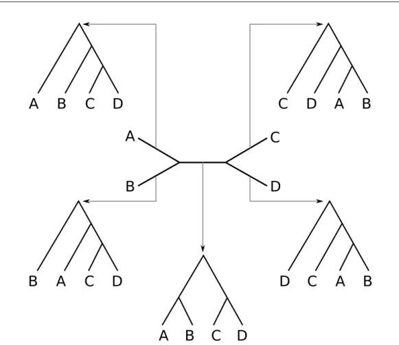
Other characteristic of trees is that they might or not contain a root node providing an evolutionary direction. According to this, we can differentiate rooted and unrooted topologies. An unrooted tree representation for N taxa is a graph with N tip or leaf nodes with degree 1, and N-2 inner nodes with degree 3. These structures provide information about the relationships between the species, but no direction is given. Given two inner nodes we cannot decide which one is older. Since most popular substitution models consider the evolution as a time-reversible process, it makes sense to work with such structures. Figure 1.2 shows an example of a 4-taxa unrooted tree. Starting from such a topology, we can root the tree at any of the branches. Usually an outgroup (a taxon clearly distant from every other) is included in the analysis in order to determine where to place the root for the group of interest, or ingroup.
A
B
D
C
B
A
C
D
A
B
C
D
D
C
A
B
C
D
A
B
A
B
C
D
Figure 1.2: Graphic representation of an unrooted tree for 4 species (in the mid-dle). A root can be placed on any of the 5 branches, producing 5 different rooted topologies out of the same unrooted topology.
1.1.3.
Computing the Likelihood of a Tree
In 1981, Felsenstein described a Maximum Likelihood (ML) framework for modelling the process of nucleotide substitution combined with phylogenetic tree estimation [24]. As a consequence of the ML search process, applying the PLF (Phylogenetic Likelihood Function) to evaluate alternative trees dominates both the running time and memory requirements of most phylogenetic inference pro-grams.
The computation of the PLF relies on the following assumptions:
2. Evolution in different parts of the tree is independent.
3. A comprehensive tree T, including a set of branch lengthsbij.
4. A substitution model is available, and defines the transition probabilities Pi→j(b), that is the probability thatj will be the final state at the end of a branch of lengthb, given that the initial state is i.
5. The substitution model is time-reversible, that is, πjPij(b) =πiPj→i(b)
These assumptions allow us to compute the likelihood of the tree as the product of the site-likelihoods of each column i of the MSA with n columns, as shown in Equation 1.4. LetT be a (rooted or unrooted) binary tree withn tips. Letθ be a set of (optimized or given) substitution model parameters (see Section 1.1.1). Let φ={bxy}be a set of (optimized or given) branch length values for tree T , where bxy is the branch length value connecting nodesxand yin tree T (bxy =byx, x6=y and |φ|= 2n−3).
L=P r(D|T, θ, φ) = n
Y
i=1
P r(Di|T, θ, φ) (1.4)
Likelihood scores usually reach very low values, that are either impossible or very computationally expensive to represent with current computer arithmetic. In order to resolve these problems, it is common practice to compute and report log likelihood values:
log(L) = log(P r(D|T, θ, φ)) = n
X
i=1
log(P r(Di|T, θ, φ)) (1.5)
For clarity, let us assume that we are working with a rooted tree and DNA data, where we have an alphabet of size four. Thus, only four states are possible and correspond to the nucleotides A, C, G, and T. For each site i, four entries must be computed to store the conditional, or marginal likelihood for nucleotide states ’a’, ’c’, ’g’, and ’t’ at node p. The conditional likelihood entryL(xp)(i) is the probability of everything that is observed from nodepon the tree towards the tips, at site i, conditional on node phaving state x[26]. We can define the conditional likelihood vector (CLV) at node p and sitei as:
~
L(p)(i) = L(ap)(i), L(p)
c (i), L(gp)(i), L (p) t (i)
(1.6)
L(xp)(i) = t
X
y=a
Px→y(bqp)L(xq)(i)
! t
X
x=a
Px→y(brp)L(xr)(i)
!
(1.7)
p
q
r
clv
rclv
qclv
ptowards root
towards tips
P(b
rp)
P(b
qp)
Figure 1.3: Conditional likelihood vectore entries are computed based on the CLVs of the children nodes, the model and the transition probability matricesP(bqp) and P(brp).
The tips, which do not have any child nodes, must be initialized. Probability Vectors at the tips are also called tip vectors. In general, the sequence at the tips already have a known value for each site and therefore can be directly assigned a probability. For instance, if siteiis an ’a’, the tip vector can be directly initialized as: L(ap)(i), Lc(p)(i), L(gp)(i), L(tp)(i)
:= (1.0,0.0,0.0,0.0).
To efficiently calculate the likelihood of a given, fixed tree, we execute a post-order tree traversal that starts at the root. Via the post-post-order tree traversal, the probabilities at the inner nodes (conditional likelihood vectors, or ancestral prob-ability vectors) are computed bottom-up from the tips toward the root. This pro-cedure to calculate the likelihood is called the Felsenstein pruning algorithm [24].
L(i) =P r(Di |T, θ, φ) = t
X
x=a
πxLrootx (i) (1.8)
For the unrooted case, the likelihood is computed at a branch instead of a node, and it is computed as shown in Equation 1.9, for sitei and the virtual root located between nodes p and q.
L(i) = t
X
x=a
πxL(xp)(i) t
X
y=a
Px→y(bpq)L(yq)(i) (1.9)
Addressing Rate Heterogeneity Among Sites
The model initially proposed by Felsenstein assumes a constant rate of substitu-tion among sites. However, this assumpsubstitu-tion has long been recognized as unrealistic, especially for genes that code for proteins or sequences that are otherwise func-tional (e.g., [89]). Since the early days of molecular data analysis, it is know that different sites or regions in DNA may evolve at different rates, or remain invari-ant [28]. The most popular method nowadays to account for rate variation among sites in nucleotide-substitution models consists in using a Γ distribution [41, 86].
In the Γ model, for each site the likelihood is integrated over a continuous Γ distribution of rates. The gamma density is given by Equation 1.10
g(r;α, β) = β
αrαe−βr
Γ(α) (1.10)
L(i) =P r(Di |T, θ, φ, α) =
However, for computational reasons, a model with equally probable cdiscrete rate categories is used instead [92]. The likelihood given each rate is computed us-ing the correspondus-ingP matrix,Pr(b), where the branch length has been properly scaled by the discrete rate (Equation 1.13).
L(xp)(i) =
Equation 1.11 is transformed into Equation 1.14, where the likelihood is the mean among all C discrete rate categories.
L(i) =P r(Di |T, θ, φ, α, C) =
The different models can also assume that a proportion of sites are invariant while others evolve at the same single rate. The per-site likelihood is the sum of the conditional per-site likelihoods assuming the site to be variant, LV, or invariant, LI For site i and the virtual root located between nodes p and q, the likelihood considering a proportion of invariant sites is computed as follows:
0 0.5 1 1.5 2 2.5 3 0
2 4 6 8
10 α= 1
α= 2 α= 20 α= 60
Figure 1.4: Probability density function of the Γ distribution
1.1.4.
Selecting the Best-Fit Model of Evolution For
Single-Gene Alignments
As it is well established, the use of one model of evolution or another may change the results of the phylogenetic analysis [18, 48, 82]. Especially, estimates of branch length or nodal support can be severely affected [13, 93]. In general, phylogenetic methods may be less accurate (recover an incorrect tree more of-ten) or may be inconsistent (converge to an incorrect tree with increased amounts of data) when the wrong model of evolution is assumed [12, 23, 38]. Because the performance of a method is maximized when it s assumptions are satisfied, some indication of the fit of the data to the phylogenetic model is necessary [37]. Indeed, model selection is not important just because of its consequences in phy-logenetic analysis, but because the characterization of the evolutionary process at the sequence level is itself a legitimate pursuit. Moreover, models of evolu-tion are especially critical for estimating substituevolu-tion parameters or for hypothesis testing [4, 85, 94, 97].
(AICc) [39, 80], or the Bayesian information criterion (BIC) [73]. All these meth-ods can also be used to test for absolute goodness of fit of the model to the data set. Other methods for model selection directed towards phylogenetic analysis are the parametric bootstrapping [31], and the decision theoretic framework [60].
Selecting the best-fit model of evolution requires the scoring of every candi-date model. Typically, this requires the optimization and evaluation of each of the competing models such that they can be compared to each other. We cannot ensure that the optimal likelihood score is achieved for each of the models, and also the optimization methods used for optimized each of the parameters (e.g., Newton-Raphson [27], Brent [76], L-BFGS-B [57]) might get stuck in local op-tima. However, in general the more thorough the models are optimized, the more accurate the selection is, marginally to the selection criteria.
Among the different statistical selection procedures, the use of sequential or hierarchical LRTs often performed poorly compared to other methods [60, 65].
Likelihood Ratio Tests
In traditional statistical theory, a widely accepted statistic for testing the good-ness of fit of models is the likelihood ratio test (LRT). LRT is based on the likeli-hood ratio, denoted by Λ (Equation 1.18).
Λ(x) = L(θ0|x) L(θ1|x)
= f(∪ixi|θ0) f(∪ixi|θ1)
(1.18)
whereL(θ1|x) is the maximum likelihood under the more parameter-rich,
com-plex model (alternative hypothesis) andL(θ0|x) is the maximum likelihood under
the less parameter-rich simple model (null hypothesis). The LRT provides the decision rule as follows:
If Λ(x)> c, do not reject H0
If Λ(x)< c, reject H0
The values c, q are usually chosen to obtain a specified significance level α, through the relation q ·P(Λ = c | H0) + P(Λ < c | H0) = α. To preserve the nesting of the models, the likelihood scores need to be estimated upon the same tree.
Likelihood ratio tests can be carried out sequentially by adding parameters (forward selection) to a simple model (JC), or by removing parameters (backward selection) from a complex model (GTR+I+Γ) in a specific order or hierarchy (hLRT). Figure 1.5 illustrates an arbitrary hierarchy of LRTs for six different models. Within each LRT, the null model is depicted above the alternative model. When the LRT is not significant, the null model (above) is accepted (A), and it becomes the null model of the next LRT. When the LRT is significant, the null model is rejected (R) and the alternative model (below) becomes the null model of the next LRT. There are six possible paths depending on the outcome of the individual LRTs, and each path results in the selection of a different model. JC: Jukes-Cantor model [42]; K80: Kimura 1980 model [49], also known as K2P; F81: Felsenstein 81 model [25]; HKY85: Hasegawa-Kishino-Yano model [35]; SYM, symmetrical model [99]; GTR: General Time Reversible model [87], also known as REV. The performance of hierarchical LRTs for phylogenetic model selection has been discussed by Posada and Buckley (2004) [65].
JC
Figure 1.5: Example of a forward hierarchy of Likelihood Ratio Tests (hLRT) for 6 candidate models
JC
JC+I JC+G F81 K80
JC+I+G F81+I K80+I F81+G K80+G HKY SYM
F81+I+G K80+I+G HKY+I SYM+I HKY+G SYM+G GTR
HKY+I+G SYM+I+G GTR+I GTR+G
Information Criteria
The Akaike information criterion (AIC, [6] is an asymptotically unbiased esti-mator of the Kullback-Leibler information quantity [70]. We can think of the AIC as the amount of information lost when we use a specific model to approximate the real process of molecular evolution. Therefore, the model with the smallest AIC is preferred. The AIC is computed as:
AIC =−2l+ 2k (1.19)
where l is the maximum log-likelihood value of the data under this model and k is the number of free parameters in the model, including branch lengths estimates. When sample size (n) is large compared to the number of parameters (say, n/k >40) the use of a second order AIC, AICc, is recommended:
AICc=AIC+
(2k(k+ 1))
(n−k−1) (1.20)
The AIC compares several candidate models simultaneously, it can be used to compare both nested and non-nested models, and model-selection uncertainty can be easily quantified using the AIC differences and Akaike weights (see Sec-tion 1.1.4). Burnham (2004) [16] provide an excellent introducSec-tion to the AIC and to model selection in general.
An alternative to the use of the AIC is the Bayesian Information Criterion (BIC) [73]:
BIC =−2l+klog(n) (1.21)
Minin (2003)[60] developed a novel approach that selects models on the basis of their phylogenetic performance, measured as the expected error on branch lengths estimates weighted by their BIC. Under this decision theoretic framework (DT) the best model is the one which minimizes the risk function:
Ci ≈ n
X
j=1
||Bˆi−Bˆj|| e
−BICj 2
PR
j=1(e −BICi
2 )
(1.22)
||Bˆi−Bˆj||2 = 2Xt−3
l=1
( ˆBil−Bˆjl)2 (1.23)
Indeed, simulations suggested that models selected with this criterion result in slightly more accurate branch length estimates than those obtained under models selected with hierarchical LRTs [60, 3].
Model Uncertainty
The AIC, BIC, and DT methods assign a score to each model in the candidate set, therefore providing an objective function to rank them. Using the differences in scores, we can calculate a measure of model support called AIC or BIC weights [15]. For the DT scores, this calculation is not as straightforward, and right now a very gross approach is used instead, where the DT weights are the rescaled reciprocal DT scores.
For example, for the ith model, the AIC (BIC) difference is:
∆i =AICi−min(AIC) (1.24)
ωi =
e−2∆i
PR
r=1(e −∆r
2 )
(1.25)
which can be interpreted, from a Bayesian perspective, as the probability that a model is the best approximation to the truth given the data. The weights for every model add to 1, so we can establish an approximate 95% confidence set of models for the best models by summing the weights from largest to smallest from largest to smallest until the sum is 0.95 [14, 15]. This interval can also be set up stochastically (see above “Model selection and averaging”).
Alfaro and Huelsenbeck studied model uncertainty in Bayesian phylogenetic analysis [7]. The BIC posterior probability appears to be more tightly distributed around the generating model, with a smaller credible interval, higher support for the best model, and higher correspondence between the best supported model and the generating model. In their paper, models in the BIC posterior distribution also more closely match the generating model in number of parameters. In contrast, the distribution of AIC-weighted models is more diffuse with lower support for any particular model, more models in the 95% credible interval, and a higher average partition distance. Notably, in a different study the distribution of AIC-weighted models seems to be biased slightly towards models of greater complexity, whereas the BIC posterior distribution of models is unbiased, or slightly biased towards less complex models [21].
1.1.5.
Selecting the Best-Fit Model of Evolution For
Multi-gene Alignments: Partitioning
goal of selecting the best-fit model for multigene or partitioned data sets is, as in the single-gene case, to find the best trade-off between model parameterization and likelihood score, according to the same criteria described in Section 1.1.4. There-fore, the model selection involves two tasks: (i) how the data should be divided (how many partitions and how they are distributed), and (ii) which substitution model is applied to each partition.
We define “data block” as a user-defined set of sites in the alignment. A data block can be, for example a particular gene, or the set of 3rd codon positions in an alignment. A “partition” (or “subset”) will be a set of one or more particular data blocks. A partition can be made of, for example, a single gene, multiple genes, or consist of the set of all first and second codon positions in an alignment. Finally, a set of non-overlapping partitions that cover the whole alignment will be called a “partitioning scheme”. Not only is important to decide which models are assigned to each of the partitions, but also how many partitions the data is divided in. The partitioning problems consists of, given a predefined set of data blocks, finding the optimal partitioning scheme for a given alignment.
For phylogenomic studies, such as the 10K vertebrate genome project [40] (http:// www.genome10k.org/) and the 1,000 insect transcriptome evolution project [61] (http://www.1kite.org/), partitioning is part of the routine analyses. However, the number of different possible choices between considering one unique partition for the entire data and one partition per data block present an exponential growth according to the number of initial data blocks, and finding the best-fit partitioning scheme among them is NP-Hard.
Let X be the data, D=d1, .., dN a collection of N non-overlapped data blocks (or subsets of X), andSthe powerset ofD. Apartitioning schemeis a subcollection
S∗ of
S such that each element in X is contained in exactly one subset in S∗ (i.e.,
each element in X is covered by exactly one subset in S∗). Mathematically, a
partitioning scheme is an exact cover of X [44]. Sk is a family of P(S) containing
all k-subsets P(S)k, such that
S
s ∈ S(s) = D ∧(s1∩s2 ={φ},∀s1, s2 ∈ S) (the
disjoint union of its elements is D). The cardinality ofSk is|Sk|=
(
N k
)
The number of different partitioning schemes for N data blocks is given by the Nth Bell number, which is the sum from 1 to N of the Stirling Numbers of the Second Kind:
The number of partitioning schemes grows very quickly. For example, for 20 data blocks there are 5.8×10¹² different partitioning schemes. For 100 data
blocks there are 4.75×10115 different possible ways to arrange the data blocks into
partitions that cover the entire data without overlapping. This number is around 1030times greater than the estimated number of atoms in the observable universe.
Finding the best-fit partitioning scheme and assigned models is a very com-putational and memory intensive task. It is also NP-Hard and therefore finding the absolute optima is not feasible even for a not so large number of single parti-tions or data blocks. The number of possible combinaparti-tions grows asymptotically to ((0.792n)/ln(n+ 1))n [9].
For k groups in each scheme, it is necessary to perform the selection for those groups with N −k + 1 data blocks. The number of combinations of k elements without repetition in a set of N elements is given by Nk, and therefore the total number of required partition evaluations will be PNi=0 ki, that equals (2N)−1 (Newton binomial theorem), giving a computational complexity of O(2N). Fig-ure 1.7 shows an example of all possible partitioning schemes for N = 4.
S(4,4)
1 2 3 4
S(4,3)
5 5 3 4
6 2 6 4
7 2 3 7
1 8 8 4
1 9 3 9
1 2 10 10
S(4,2)
5 5 10 10
6 9 6 9
7 8 8 7
11 11 11 4
12 12 3 12
13 2 13 13
1 14 14 14
S(4,1)
15 15 15 15
Figure 1.7: Partitioning schemes for N = 4. Numbers and colors represent the different partitions. In this example, there are 2N−1 = 15 partitions andB(N) = 15 partitioning schemes.
Given these 2N−1 partitions, we can think the best-fit partition search problem as the set cover problem [88] where each partition is given a weight (i.e., the BIC score). Our target is to find the k non-overlapped subsets covering the whole alignment that minimizes the score. The set cover problem is NP-Hard [51], so it is the best-fit partition selection as well.
The set of disjoint partitioning schemes that contains every different possible partition is given by those combinations obtained from the subset S1∪ S2.
Par-titions included in every other partitioning scheme will appear in one single par-titioning scheme from the subset described before. In the example in Figure 1.7, the setsS1 andS2 contain all possible partitions, and for eachs∈ S3∪ S4, there is
exactly 1 elementx∈ S1∪ S2 such thatx∈s. This subset has cardinality 2N−1, and as long as every element butS1includes exactly 2 partitions, the total number
Going a step further, we can also link parameters across partitions, slightly reducing the total number of parameters, but also increasing the complexity and thus making the best-fit scheme selection much harder.
At the genomic scale the heterogeneity of the substitution process becomes even more apparent that at the single-gene scale, as different genes or genomic regions can have very different functions and evolve under very different constraints [8]. Multilocus substitution models that consider distinct models for different parti-tions of the data assumed to evolve in an homogeneous fashion have been proposed under the likelihood [69, 95] and Bayesian [63, 79] frameworks. In this case, differ-ent loci (or loci by codon position) are typically considered as distinct partitions by default, without further justification, like for example the set of 1st, 2nd or 3rd codon positions in protein-coding sequence alignments [75] or distinct protein domains [100]. However, a number of empirical studies have demonstrated that different partitioning schemes can affect multilocus phylogenetic inference, includ-ing tree topology, branch lengths and nodal support [10, 43, 55, 68, 90], with maximal differences occurring when whole datasets are treated as single partitions (i.e., unpartitioned). Using computer simulations, Brown and Lemmon (2007) showed that both over and particularly under-partitioning can lead to inaccurate phylogenetic estimates [11].
The most popular tool for automatic statistical selection of partitioning schemes for multilocus data sets is PartitionFinder [53], released in 2012. PartitionFinder is written in Python, and makes an intensive use of external software such as PhyML [33] or RAxML [77] for the phylogenetic inferences and model optimiza-tion. It uses combinatorial optimization heuristics, like hierarchical clustering and greedy algorithms building up on previous ideas raised by Li et al. [56].
1.2.
Software for Model Selection
1.2.1.
ProtTest 2.x
data set. Instead, replacement rates previously estimated from large empirical databases are adopted. Among these, some of the more popular are the Day-hoff [22], JTT [32], mtREV [5], WAG [91], mtArt [1] or LG [54] matrices. Impor-tantly, many phylogenetic calculations like the estimation of tree topologies, branch lengths, nodal support, divergence times or replacement rates benefit from the use of explicit models of evolution. Because the use of different models can change the outcome of the analysis [81], different model selection tools for protein alignments have been implemented in the past, like ProtTest [2], Model-Generator [46] or TOPALi [59].
ProtTest is one of the most popular tools for selecting models of protein evo-lution, with more than 2,000 citations. ProtTest is written in Java and uses the program PhyML [34, 33] for the ML estimates of phylogenetic trees and model parameters. The candidate set of models contain 14 different rate matrices that result in 112 different models when we consider rate variation among sites (+I: invariable sites; +G: Γ-distributed rates) and the observed amino acid frequencies (+F). ProtTest uses the selection criteria described in Section 1.1.4 to find which of the candidate models best fits the data at hand. In addition, it can perform multi-model inference and estimate parameter importances [65]. The time required to complete the likelihood calculations, that take most of the runtime of the pro-gram, can be variable depending on the size and complexity of the alignments and models. For large alignments, this task cannot be completed in a reasonable time using a single core. While ModelGenerator/MultiPhyl [47] and TOPALi imple-ment grid computing to speed-up the analyses, they consider fewer models and do not implement model averaging. Also grid implementations usually include a very large overhead compared to HPC-oriented architectures.
1.2.2.
ModelTest and jModelTest 1.x
BIC). It is written in Java, and makes use of PhyML for phylogenetic calculations.
jModelTest supports 88 submodels of the general time-reversible model. On top of 11 different substitution schemes and stationary frequencies (Table 1.2), each of these models can assume rate variation among sites (+I: invariable sites; +G: Γ-distributed rates).
Table 1.2: Substitution models available in jModelTest.
Model Free Base Substitution Rates Substitution
Parameters Frequencies Code
JC k Equal AC = AG = AT = CG = CT = GT 000000
F81 k + 3 Unequal AC = AG = AT = CG = CT = GT 000000
K80 k + 1 Equal AC = AT = CG = GT, AG = CT 010010
HKY k + 4 Unequal AC = AT = CG = GT, AG = CT 010010
TrNef k + 2 Equal AC = AT = CG = GT, AG, CT 010020
TrN k + 5 Unequal AC = AT = CG = GT, AG, CT 010020
TPM1 k + 2 Equal AC = GT, AT = CG, AG = CT 012210
TPM1uf k + 5 Unequal AC = GT, AT = CG, AG = CT 012210
TPM2 k + 2 Equal AC = AT, CG = GT, AG = CT 010212
TPM2uf k + 5 Unequal AC = AT, CG = GT, AG = CT 010212
TPM3 k + 2 Equal AC = CG, AT = GT, AG = CT 012012
TPM3uf k + 5 Unequal AC = CG, AT = GT, AG = CT 012012
TIM1ef k + 3 Equal AC = GT, AT = CG, AG, CT 012230
TIM1 k + 6 Unequal AC = GT, AT = CG, AG, CT 012230
TIM2ef k + 3 Equal AC = AT, CG = GT, AG, CT 010232
TIM2 k + 6 Unequal AC = AT, CG = GT, AG, CT 010232
TIM3ef k + 3 Equal AC = CG, AT = GT, AG, CT 012032
TIM3 k + 6 Unequal AC = CG, AT = GT, AG, CT 012032
TVMef k + 4 Equal AC, AT, CG, GT, AG = CT 012314
TVM k + 7 Unequal AC, AT, CG, GT, AG = CT 012314
SYM k + 5 Equal AC, AG, AT, CG, CT, GT 012345
1.3.
Scope and Motivation
As mentioned before, the use of different models of substitution can change the results of the phylogenetic analysis. Tools for automated selecting the best-fit model of evolution under a Maximum-Likelihood framework exist from the late 90s and they are continuously improving [2, 45, 66].
However, the irruption of Next-Generation Sequencing technologies (NGS) has caused a data avalanche in recent years. The growing rate at which molecular data is being available for researchers encourages the need of developing faster analysis methods. Moreover, it is common in most research groups in the field to have access to local or remote HPC architectures. Thus, HPC and fault tolerance techniques are of great importance.
On top of that, also due to the data explosion, the study of genomic data has become more popular in the last years. Different regions of the genome can evolve in a very different way, and therefore the old approach of analysing the whole data with a single model became obsolete. Selecting the best-fit partitioning scheme (i.e., the best scoring one) is a very computational expensive and memory intensive task, and finding the absolute optima is not feasible for a not so large number of single partitions or genes.
1.4.
Main Objectives of the Thesis
The main goal of this thesis is the improvement and evaluation of the existing techniques for selecting the best-fit model of nucleotide substitution and amino acid replacement for single and multigene sequence alignments.
reference for model selection: jModelTest and ProtTest. Evaluating the perfor-mance of different selection criteria involves testing the accuracy recovering the model parameters out of a set of simulated data, where the true generating model is known.
ProtTest 3: Fast Selection of
Best-fit Models of Protein
Evolution
The content of this chapter corresponds to the following journal paper:
Title: ProtTest 3: Fast selection of best-fit models of protein evolution
Authors: Diego Darriba, Guillermo L. Taboada, Ram´on Doallo and David Posada
Journal: Bioinformatics
Editorial: Oxford University Press, ISSN: 1367-4803, EISSN: 1460-2059
Year: 2011
Volume(Number):Pages: 27(8):1164–1165
DOI: 10.1093/bioinformatics/btr088
Impact factor: 4.981
Q1; 10th position on Computer Science Applications, 35th position on Molec-ular Biology
Number of citations: 547 as of October 2015
The final publication is available at
http://bioinformatics.oxfordjournals.org/content/27/8/1164.full.
ProtTest 3: fast selection of best-
fi
t models of protein
evolution
Diego Darriba1,2, Guillermo L. Taboada2, Ram ´on Doallo2, David Posada1∗ 1Department of Biochemistry, Genetics and Immunology, University of Vigo, 36310 Vigo, Spain 2Computer Architecture Group, University of A Coru ˜na, 15071 A Coru ˜na, Spain
ABSTRACT
Summary:We have implemented a High Performance Computing
(HPC) version of ProtTest (Abascalet al., 2007) that can be executed in parallel in multi-core desktops and clusters. This version, called ProtTest 3, includes new features and extended capabilities.
Availability:ProtTest 3 source code and binaries are freely available
under GNU license for download fromhttp://darwin.uvigo.es/ software/prottest3, linked to a Mercurial repository at Bitbucket (https://bitbucket.org/).
Contact:[email protected]
Supplementary information:Supplementary data are available at
Bioinformatics online.
1 INTRODUCTION
Recent advances in modern sequencing technologies have resulted in an increasing capability for gathering large data sets. Long se-quence alignments with hundred or thousands of sese-quences are not rare these days, but their analysis imply access to large computing infrastructures and/or the use of simpler and faster methods. In this regard, High Performance Computing (HPC) becomes essential for the feasibility of more sophisticated –and often more accurate– anal-yses. Indeed, during the last years HPC facilities have become part of the general services provided by many universities and research centers. Besides, multicore desktops are now standard.
The program ProtTest (Abascalet al., 2007) is one of the most
popular tools for selecting models of amino acid replacement, a routinary step in phylogenetic analysis. ProtTest is written in Java and uses the program PhyML (Guindon and Gascuel, 2003) for the maximum likelihood (ML) estimation of model parameters and phylogenetic trees and the PAL library (Drummond and Strimmer, 2001) to handle alignments and trees. Statistical model selection can be a very intensive task when the alignments are large and include divergent sequences, highlighting the need for new bionformatic tools capable of exploiting the available computational resources.
Here we describe a new version of ProtTest, ProtTest3, that has been completely redesigned to take advantage of HPC
environ-ments and desktop multicore processors, significantly reducing the
execution time for model selection in large protein alignments.
2 PROTTEST 3
The general structure and the Java code of ProtTest has been com-pletely redesigned from a computer engineering point of view.
∗to whom correspondence should be addressed
We implemented several parallel strategies as distinct execution
modes in order to make an efficient use of the different computer
architectures that a user might encounter:
(1) a Java thread-based concurrence for shared memory architec-tures (e.g., a multi-core desktop computer or a multi-core cluster node). This version also includes a new and richer Graphical User Interface (GUI) to facilitate its use.
(2) an MPJ (Shafiet al., 2009) parallelism for distributed memory
architectures (e.g., HPC clusters).
(3) a hybrid implementation MPJ - OpenMP (Dagum and Menon, 1998) to obtain maximum scalability in architectures with both shared and distributed memory (e.g., multicore HPC clusters).
Moreover, ProtTest 3 includes a number of new and more
com-prehensive features that significantly extend the capabilities of the
previous version: (1) moreflexible support for different input
align-ment formats through the use of the ALTER library (Glez-Pe˜na
et al., 2010): ALN, FASTA, GDE, MSF, NEXUS, PHYLIP and PIR; (2) up to 120 candidate models of protein evolution; (3) four
strate-gies for the calculation of likelihood scores:fixed BIONJ, BIONJ,
ML or user-defined; (4) four information criteria: AIC, BIC, AICc
and DT (see Sullivan and Joyce 2005); (5) reconstruction of model-averaged phylogenetic trees (Posada and Buckley, 2004); (6) fault tolerance with checkpointing; and (7) automatic logging of the user activity.
3 PERFORMANCE EVALUATION
In order to benchmark the performance of ProtTest 3, we computed the running times for the estimation of the likelihood scores of all 120 candidate models from several real and simulated protein align-ments (Table 1). When these data were executed in a system with shared memory, e.g., a multicore desktop, the scalability was almost linear as far as there was enough memory to satisfy the require-ments. For example, in a shared memory execution in a 24-core node the speedup was almost linear with up to 8 cores, also scal-ing well with data sets with medium complexity, like HIVML or COXML (Fig. 1). In a system with distributed memory like an clus-ter, the application scaled well up to 56 processors (Fig. 2). With more processors a theoretical scalability limit exists due to the het-ereogeneous nature of the optimization times, from a few seconds for the simplest models to up to several hours for the models that include rate variation among sites (+G). This problem was solved with the hybrid memory approach. In this case, the scalability went beyond the previous limit, reaching up to 150 in the most complex cases with 8-core nodes (Figure 3).
1 Associate Editor: Prof. Martin Bishop
© The Author (2011). Published by Oxford University Press. All rights reserved. For Permissions, please email: [email protected]
at 62324608-Swets. Subs. Service on May 15, 2014
http://bioinformatics.oxfordjournals.org/