Flexible Scheduling in a CPG Company

Texto completo

(1)Información Importante. La Universidad de La Sabana informa que el(los) autor(es) ha(n) autorizado a usuarios internos y externos de la institución a consultar el contenido de este documento a través del Catálogo en línea de la Biblioteca y el Repositorio Institucional en la página Web de la Biblioteca, así como en las redes de información del país y del exterior con las cuales tenga convenio la Universidad de La Sabana. Se permite la consulta a los usuarios interesados en el contenido de este documento para todos los usos que tengan finalidad académica, nunca para usos comerciales, siempre y cuando mediante la correspondiente cita bibliográfica se le de crédito al documento y a su autor. De conformidad con lo establecido en el artículo 30 de la Ley 23 de 1982 y el artículo 11 de la Decisión Andina 351 de 1993, La Universidad de La Sabana informa que los derechos sobre los documentos son propiedad de los autores y tienen sobre su obra, entre otros, los derechos morales a que hacen referencia los mencionados artículos.. BIBLIOTECA OCTAVIO ARIZMENDI POSADA UNIVERSIDAD DE LA SABANA Chía - Cundinamarca.

(2) Flexible Scheduling in a CPG Company Natalia Ardila† Alejandro Perez Santillan† Francisco Tablado† † GCLOG Program 2014 – MIT Global SCALE Network Boston, Massachusetts – United States Email: [email protected], [email protected], [email protected] Universidad de La sabana, Bogota – Colombia Universidad Torcuato Ditella, Buenos Aires - Argentina. Abstract– In fast growing markets like Latin America, supply networks are required to be flexible and responsive while keeping low inventory levels. The scope of this project is to identify key variables that could help a CPG company significantly reduce the Days Between Next Run (DBNR) metric, and to develop a model or process to assess and test how changing these variables would impact the production cycle and the associated inventory levels reducing the need for safety stock in the whole supply chain. By applying rescheduling model runs with high volume or long cycle time that affect the measure of DBNR will be reduced by split them achieving a reduction of current metric form 12 to 9 Days Between Next Run in the plant. 1. Introduction Oral Care (toothpaste, toothbrushes) is a fastgrowing business for this CPG Company in Latin America and these supply networks required being flexible and responsive (zero out of stocks) while keeping low inventory levels. The CPG Company has different sourcing through the world to supply most of 15 Latin America locations, one of the main sourcing plants and main focus of this project is the plant of Mexico which supplies a large part of the Latin American market. The Sourcing plant processes are show in Exhibit 1, the processes are split in three main parts Making, Packing and Customization, and it. GCLOG 2014. will focus on packing process where the main variables are taking in consideration.. Fig 1. Sourcing plant - Overall Process. Virtually the focus of all manufacturing plants is to find the balance between on-time deliveries, short customer lead times, cycle times and maximum utilization of resources. One of this variables associate to cycle times is the DBNR (Day Between Next Run), that assess how often a material is produced over a given time frame (better indicator than ‘cycle time’) This measure according CPG company DBNR (2013) has different focus: (i) Number of calendar days from time a production run of a material ends until the next production run of the same material is started, same SKU (ii) A production run is defined as period of time where production of a material occurs on consecutive days (iii) Calculation uses a production volume weighted average on a stat case basis by plant by material code by calendar day (iv) It is a rolling three-month measure, calculated across a three-month time frame, reported monthly for the total business. Reporting is delayed by 30 days, to allow for the data collection to occur for last runs in the period The total DBNR of plant could be expressed as:.

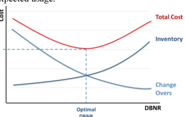
(3)  q  Plant DBNR   DBNR i  i  Q i  Formula 1: DBNR calculation. Where i correspond the number of production lines from i =1..,5, qi the demand of line sub i and Q the total demand of the plant. Moreover, other variable associated to maximum utilization of resources is the PR (PR – Overall Equipment Effectiveness), measure that takes in consideration 3 types of variables expressed under a Loss Tree  Quality Loss  Target Rate Loss  Not at Target Speed o Planned Losses o Unplanned Losses The ones over the scope of this project will have direct impact are:  Not at Target Speed o Planned Losses  Buggie Changeover  Lot Changeover  Version Changeover  Size Changeover Then to calculate the total PR per plant is used the following formulas: Per line is calculating a PR:. PRtotal  PDT Actual Line % total .  UPDT Actual Line % total    Quality Loss % total  T arg et Rate Loss % total Formula 2: PR Total. In the case of any decrease over DBNR the PR tends to increase; here exist a challenge due to increase the runs of different SKU in production reduce the performance of the lines over their expected usage.. Graphic 1. Optimal DBNR. The optimal DBNR will be get as a tradeoff between number of changeovers affecting the PR of the plant and the inventory levels of the same, tools as scheduling planning, opps and changeover utilization made the desire result possible to achieve. Gap vs. Plan Actual  Plan PDT Actual Line %  Gap vs. Plan PR  PDT Actual Line %   UPDT Actual Line % .  Quality Loss %   T arg et Rate Loss % Formula 2: PR per Line i. Then the total PR of plant is calculated as follows: Gap vs. Plan x Vol Actualline ( i ) Gap vs. Plantotal  Total Vol Packing. PDT Actual Line % total  Gap vs. Plan total. GCLOG 2014. 2. Literature Review According Pinedo (2009) the scheduling process also interacts with the production planning process, which handled medium – to long term planning for the entire organization. Achieving a correct planning process within and scheduling process the plant will be available to impact the entire operation. This scheduling optimization is base in inventories level, demand forecast, and resource requirements this interaction is shows under Exhibit 2, where the correct flows of information in the manufacturing system is denoted..

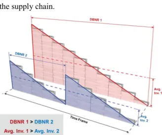
(4) variability, makes planning processes easier reducing the levels and need for safety stock in the supply chain.. Fig 1. Detailed Scheduling. Modern factories as the case of this company, employ elaborate manufacturing information systems involving a computer networks and various data bases, as input of this systems demand planning files and MRP (Material Requirements Planning) are using in order to get the correct scheduling planning, as output tools as ERP (Enterprise Resources Planning), helps the company to get the monthly or weekly scheduling for the plant. The efforts of this capstone will be focus on rescheduling process, in order to accomplish one of variable, not including as restriction during the planning scheduling made by the ERP, the DBNR without compromise the PR of the plant. For this reason is important take in consideration the impact of cycle time over scheduling planning and overall performance of the plant. According Kimpf et al. (2009) in a make to stock company, cycle time is important because long cycle times lead to an increased risk of product quality due to the fact that it will generally take long to detect manufacturing problems. If any manufacturing problem is detected under MTO company shorter cycle times allow them to reduce reject products. Additionally, as an overall view as company, the mean and variability of product cycle times is important as they impact the amount of safety stock that must held, reducing the inventories levels over the complete supply chain, but is important not only lead efforts to make shorten average cycle times but also accurately estimate cycle times and reduce cycle time variability. Kimpf et al. (2009) mentioned that accurate cycle time estimation results in a more stable production environment reducing cycle time. GCLOG 2014. Fig 2: Reducing Cycle times (DBNR). Here is where the main objective of this capstone project is taking in consideration reduce the cycle time knowing as DBNR as driver to decrease the inventory in the whole supply chin of the company.. 3. Methodology and Data Analysis. Fig 3: Methodology. After literature reviewing to get a deeply knowing of planning and scheduling tools and the visit to the plant it will analyze the data provided by the company. Below we will show few scenarios where the decrease of the DBNR per interval, affect the total DBNR: It has made a simple example where have been take 4 items with and average cycle time:.

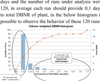
(5)  q  Plant DBNR   DBNR i  i  Q i  5 20 30 45 100   12  9 7 100 100 100 100 5  2.4  2.7  3.15 13,25 Fig 2. Example DBNR of plant. Once the DBNR is calculated, what if we decrease in 1%:. also that runs with high volume or long cycle time affect the measure of DBNR. The run “i” has a relatively HIGH DBNR.  q  Plant DBNR   DBNR i  i  Q i . Example: SKU XY1 - June 6th, 2013 Volume: 12.96 Q - DBNR: 71 days Impact on Plant DBNR: 71*12.96/785.38=1.17 9.8% of the Plant DBNR The run “i” has a relatively high volume.  q  Plant DBNR   DBNR i  i  Q i . Fig 3. Decrease 1%. what if Decrease 20%. Fig 4. Decrease 20%. We will focus our analysis in a 90 days run provided by the plant, the initially measure is 12 days and the number of runs under analysis were 120, in average each run should provide 0,1 days to total DBNR of plant, in the below histogram is possible to observe the behavior of these 120 runs.. Histogram 1: Average weight DBNR per run. Is possible to observe that 75.61% of these run accomplish the target, but the 24% (30 runs) increase the metric of total DBNR. It will notice. GCLOG 2014. Example: SKU XY2 - August 12th, 2013 Volume: 103.83 Q - DBNR: 5 days Impact on Plant DBNR: 5*103.83/785.38=0.66 5.54% of the Plant DBNR The efforts will be focus on split runs with high volumes, below it shows the VBA model run in excel to reduce the DBNR increasing the number of runs in the plant Const step = 100 Const minQty = 3 Const speed = 8333 Public Function lotSize(forecast As Variant, DBNR As Variant, minCorr As Variant) As Double lotSize = 0 For lot = 100 To forecast Step step days = Int(lot / speed) + 1 qty = Int(forecast / lot) + 1 totalDays = qty * (days + DBNR) If (totalDays > 85) And (totalDays < 95) And (qty >= 3) Then lotSize = lot End If Next If lotSize = 0 Then lotSize = forecast / minCorr End If End Function Model 1: VBA lot size model. 5. Results.

(6) Once the target is estimated, the program adjusts the number of runs to fit the target based on reducing cycle times between same SKU’s. Based on this model where the main function optimization is to reduce and achieve a DBNR of 9 days the plant will run 160 runs instead off 120 initial runs. Fig 5. Results after model. Reducing the weight of each run to 0,257 weighted DBNR per SKU the plant will be achieve the target of 9 days, quantitative components as this plus qualitative components as grouping of top 10 SKU that contribute more weight to the quarterly measure. A suggested schedule for plant, per SKU analyzed will be shown by the template in order to give a graphical approach to the company.. GCLOG 2014. Fig 6. Suggested Weekly schedule. 6. Conclusion In this case is important to include into the “Cedula” weekly planning a model to estimate the DBNR metric, key variable for the company. In this case is essential to considering not only quantitative but also qualitative methods components, in order to provide a guideline for future planning. Also the graphic approach gave to the company a visual planning adherence to determine the level of variability acceptable. Cycle time is a measure to decrease security stock and inventory levels, due long lead times from plant located in Central America to the rest of markets located mainly in South America, a reduction in few days don’t impact the total inventories level over the whole supply chain..

(7) References CPG company DBNR presentation, November 2013 Watson, M., Lewis, S., Cacioppi, P., Jayaraman, J:, 2012, “Supply Chain Network Design: Applying Optimization and Analytics to the Global Supply Chain” Shapiro, J.F., 2009, “Modeling the Supply” Chopra, S.,Meindl, P. 2012, Supply Chain Management: Strategy, planning and Operation, Ghiani, G., Laporte, G., Musmanno, R,. “Introduction to Logistics Systems Planning and Control” Fisher, M.L., and Jaikumar, R. (1981), "A generalized assignment heuristic for vehicle routing", Networks 11, 109-124. Baisley J.E (1982) “Route First – Cluster Second Methods for Vehicle Routing” Pinedo, Michael L., 2009, “Planning and Scheduling in Manufacturing and Services” Kempf, Karl G, Keskinocak, P., Uszoy, R., Planning Production and Inventories in the Extended Enterprise.

(8) Exhibit 1. Flowcharts General Process.

(9) Making Process.

(10) Packing Process.

(11) Customization.

(12) Exhibit 2. Information flow Diagram.

(13)