Reaching social consensus family budgets:
The Spanish case
J.M. Casc´ona, T. Gonz´alez-Arteagab, R. de Andr´es Callec,∗
aDepartment of Economics and Economic History,
Institute on Fundamental Physics and Mathematics University of Salamanca, E37007 Salamanca, Spain
bBORDA and PRESAD Research Groups and
Multidisciplinary Institute of Enterprise (IME), University of Valladolid, E47011 Valladolid, Spain
cBORDA Research Unit, PRESAD Research Group and
Multidisciplinary Institute of Enterprise (IME), University of Salamanca, E37007 Salamanca, Spain
Abstract
The study of family budgets has been traditionally used to analyse consumers’ behaviour and estimate cost-of-living since the end of 19th century. Generally speaking, the computation of the budgets has been based on two different method-ologies, the prescriptive and the descriptive method. Both present several draw-backs like the comparison among different areas, family types and over time.
This paper proposes a new methodology for reaching family budgets, namely
social consensus family budgets, to overcome such problems and examine the main features of the novel approach. The suggested method uses the minimiza-tion of the differences with respect to the consumer’s preferences to obtain a so-lution that summarizes single behaviour into a social preference. This approach is especially conceived for preferences on possibly related-expenditure groups. In addition, several algorithms are introduced to compute the social family bud-gets. Finally, the contribution includes the Spanish case as an example of reaching some social consensus family budgets in order to show the operational character and intuitive interpretation of the proposal approach.
∗Corresponding author
Email addresses:[email protected](J.M. Casc´on),
Keywords: Ordinal information codification, Social consensus solution,
Correlation, Recursiveα-index algorithm, Family budgets, Expenditure groups
1. Introduction
Taking a decision means select among several alternatives. When decision depends only on the opinion of one person, its study is related toRational Deci-sion Making Theory. If decision depends on a group of people, the process adds a layer of complexity and its study is included in Group Decision Making The-ory. A group decision making problem involves, basically, a set of individuals and set of available alternatives. Under these simple assumptions, each individual expresses her/his preferences on alternatives and the problem is solved when indi-vidual’s preferences are mixed in a group’s preference1. Generally speaking, the achievement of an overarching solution has been considered like an aggregation problem from Borda [4], Kendall [5] (in a voting context) to Saari and Merlin [6], Meskanen and Nurmi [7], Klamler [8, 9] and de Andr´es Calle, Garc´ıa-Lapresta and Gonz´alez-Pach´on [10] (using distance-based aggregation rules).
Nowadays, obtaining of a group’s preference entails not only aggregating but also finding the best alternative or the solution that more consensus conveys among decision-makers. Due to this fact, there has been an increasing interest in developing approaches to solve this new paradigm in this kind of problems like
goal programming techniques [11], operational procedures [12], cluster models [13],p-indicators [14], multi-objective programming theories [15], control strate-gies [16] and conditional probabilities [17], among others.
This paper is focused on the contribution of Gonz´alez-Arteaga, Alcantud and de Andr´es Calle [18] which proposes a distance-based methodology to obtain group consensus solutions, namelyMahalanobis social consensus solutions. This particular methodology is especially designed for correlated alternatives and ob-tains group solutions minimizing the dissensus among individual’s preferences2. However, it is needed to stress that the main weakness of the approach presented in [18] is its computational complexity even for a small set of alternatives3. In
1Preferences on alternatives can be expressed by means of different types of preference
rela-tions such as ordinal [1], linguistic [2], multiplicative [3], and so on.
2The paper is focused on preferences on alternatives express by means of complete preorders. 3In group decision making context, persons’ maximum efficiency on one-dimensional absolute
particular, the formulated optimization problem can be tackled by a force-brute attack, but this strategy must be rejected because the cardinality of the set of all complete preorders on the alternatives set grows dramatically in terms of the num-ber of alternatives.
Taking into account the aforementioned limitations, the objectives of this re-search are to improve and to extend the proposal of [18], by means of designing a strategy to compute efficiently Mahalanobis consensus solutions, particularly when the number of alternatives is not small. To achieve these goals, the central thesis of this paper is to writte the optimization problem presented in [18] as a set ofmixed-integerquadratic programming problems and solve them, assuming that they are NP-hard decision problems [20]. Then, this primary aim is divided into three main research contributions:
• Firstly, prior to transform the original problem into mixed-integer quadratic problems, thecanonical codification included in [18] to codify ordinal in-formation must be adapted due to the feasible set wich is determined by equality linear constraints using continuous and binary variables. There-fore, the concept ofα-indexis introduced as well as the characterization of the canonical codified complete preorder based on theα-index.
• Secondly, the feasible set is setted by means of a novel recursive algorithm, the Recursiveα-index algorithm (RAI). As has already been evoked, one of the main obstacles in the resolution of this type of optimization problems is the setting of the feasible set for a “not small” set of alternatives. To be precise, the number of preorders on a set of k alternatives is equal to
Pk
j=0j!·S(k, j),beingS(k, j)the Stirling number of the second kind
4. To our knowledge, there is not a procedure to determine feasible set on set of preorders in the specialized literature5.
• Finally, an algorithm to efficiently compute Mahalanobis consensus solu-tions, theMahalanobis consensus solution algorithm(MCSA), is defined.
In closing and with the goal of putting in practice the aforementioned re-searches, this study aims to contribute to this growing area of research by propo-sing a new methodology to compute family’s budgets and then analyse consumers’
4see [21] and The On-Line Encyclopedia of Integer SequencesR (OEISR) Wiki,http:// oeis.org/A000670
5In [22] there is another procedure to compute the number of preorders associated to a set of
behaviour. In these times of a new global economy, consumers’ preferences are changing all the time (modifications in living standards, tendency, technology, et cetera) and the establishment of consumers’ behaviour patterns is a key re-search area. The study of consumers’ preferences and their behaviour is one of the greatest challenges for companies because product marketing is largely de-pendent on them (see [23], [24] and [25], ammong others) and for Governments because the efficacy and efficiency of public policies (regulatory, welfare, etc.) is also dependent on them (see [26]). Therefore, this paper sets out to investigate the usefulness of the proposed methodologies to determine consumers’ preferences and the ranking of those expenditure groups that best agrees with family pref-erences. That is, the ranking that minimizes the disagreement among families’ ranking expenditure groups considering the relation among expenditure groups. Specifically, the focus of the work is on the Spanish Economy. Based on Spanish data on household budgets from 2016, the ranking of the expenditure groups for the Spanish consumers, i.e., the Spanish consumers’ behaviour by the year 2016, is obtained by means of the proposed methodologies. Among other research con-sequences, getting Spanish consumers’ behaviour patterns will allow companies and also the Spanish Government to improve their marketing and public policies, respectively.
This paper is organized as follows. Section2introduces some starting points like notation and basic definitions. In Section 3, the main research contributions of this paper to compute efficiently Mahalanobis consensus solutions are intro-duced. Section 4 includes the real case of study on Spanish Economy to obtain family budgets. This section analyses the results obtained and provides discus-sions on them. Finally, some concludiscus-sions and further research work are presented in Section5.
2. Starting points
Prior to commencing the study, this section reviews some previous definitions as well as the approach proposed by Gonz´alez-Arteaga, Alcantud and de Andr´es Calle [18] to obtain social consensus solutions under the possibility of alternatives correlated.
2.1. Notation
Let us denote by N = {1,2, ..., n}, n > 1 a society of individuals and by
the cardinality ofXis at least 2, |X| > 2. For simplicity of notation, we writes
instead of issuexs.
Without loss of generality it is required that experts rank alternatives by means of complete preorders6. Centring on reflecting real situations, the representation of agents’ opinions allows ties among alternatives7. W(X)denotes the set of all complete preorders onX.
Let R ∈ W(X) be a complete preorder on X, then xi R xj means xi is strictly preferred to xj, xi ∼R xj meansxi and xj are equally preferred and
xi <R xj means alternativexi is at least as good asxj. Any permutationπ of the alternatives{x1, . . . , xk}determines another preorder πRgiven by:
xiπRxj ⇔ xπ−1(i)Rxπ−1(j), for everyi, j ∈ {1, . . . , k}.
LetP = (R1, ...,Rn) ∈ W(X)×. . .×W(X) = W(X)n be theprofileof
N(the society) onX(the set of alternatives). TheRi ∈ P element stands for the
i-th individual’s preferences on thek alternatives for eachi= 1, ..., n.
Dealing with ordinal information like preorders, necessarily involves to esta-blish how it is represented. The first serious discussion and analysis of transform-ing or codifytransform-ing ordinal information into numerical values emerged with Borda’s work [4]. Subsequently, several procedures have been suggested to that purpose as [27], [28] and [29], among others.
The choice of a strong codification procedure is an essential issue to accom-plish any methodology on ordinal information. Therefore, the next subsection provides the codification method proposed in [18], thecanonical codificationand includes a slightly modified characterization of it.
2.2. Codification of preferences
A codified complete preorder of R ∈ W(X) is a real vector
mR = (m1, . . . , mk), being mj the codification value corresponding to alterna-tive xj and satisfyingmi ≥ mj ⇔ xi <R xj. Note that any m ∈ Rn produces a unique preorderR, however every preorder Rcan be associated with infinitely many vectorm∈Rn.
6Complete preorders or weak orders, i.e., a complete and transitive binary relation onX. 7Throughout this paper, calligraphic letters are used to denote preorders and its corresponding
Analogously, acodified profileofP = (R1, . . . ,Rn)is an×kreal matrix:
MP = (mR1, . . . ,mRn)∈Mn×k
wheremij is the codification value of agentiover the alternativexj. We denote Mn×kthe set of alln×kreal matrices.
Definition 1. Given R ∈ W(X) be a complete preorder on X, its canonical codified complete preorderis defined by the vector:
cR = (c1, ..., ck)∈({1, . . . , k})k
where cj is the number of alternatives that are graded at most as good as xj,
cj =|{q:xj <Rxq}|.
The set of all canonical codified complete preorders associated to W(X)is de-noted byF =F(W(X)).
Acanonical codified profileassociated withP = (R1, ...,RN) ∈ W(X)nis an n ×k real matrix, namely MP = (cR1, ...,cRn) ∈ Mn×k, where the row i,
denoted by cRi, represents the canonical codified complete preorder associated
withRi.
This particular codification was characterised in [18, Proposition 1]. This con-tribution includes such proposition although slightly modified. The same proof is still valid and may be omitted.
Proposition 1. A vectorc = (c1, . . . , ck) ∈ ({1, . . . , k})k is the canonical
codi-fied complete preordercRassocited withR ∈W(X)(i.e.cR∈F) if and only if
the increasingly ordered vector↑c= (c(1), . . . , c(k))satisfies:
c(k) =k. (1)
c(j) =c(j+1)−tj+1dj+1, j ∈k−1, . . . ,1. (2)
wheretj+1is the number of values equal toc(j+1)anddj+1 =
0 ifc(j+1) =c(j),
1 otherwise.
For abbreviation, a preorderRcan be identified with its canonical codification
cR, i.e.,R ≡cR.
2.3. The Mahalanobis consensus solution for ordinal information
TheMahalanobis social consensus solution provides a complete preorder Rb
that is thebest agreementtaking into consideration the Mahalanobis distance. Al-though the Mahalanobis consensus solution can be computed for any codification of preorders, our presentation is restricted to the canonical codification introduced at Subsection2.2.
First, theMahalanobis consensus distance function(MCDF) is defined. It is the objective function that must be optimized to get the consensus solution.
Definition 2. Let Σ ∈ Mk×k be a definite positive matrix. Given a profile P = (R1, . . . ,Rn) ∈ W(X)n of complete preorders and its canonical
codi-fied profile,MP = (cR1, . . . ,cRn)∈Mn×k. TheMahalanobis consensus distance
function (MCDF)is a mapping
CΣ,P :W(X)−→[0,∞)
that assigns to any complete preorderR ∈W(X)with canonical codificationcR
the real number:
CΣ,P(R) = n
X
i=1
dΣ(cRi,cR) =
n
X
i=1
(cRi −cR)Σ
−1(c
Ri−cR)
t (3)
Remark 1. IfCP,R ∈Mn×kdenotes a matriz whosei-th row iscRi−cR, we can rewrite MCDF as:
CΣ,P(R) = tr(CP,RΣ−1CPt,R), (4)
wheretr(·)is the trace operator (tr(A) = Pn
i=1aii).
Now, the Mahalanobis consensus solutioncan be introduced as the preorder that minimizes the Mahalanobis distance to a given profile. Formally:
Definition 3. TheMahalanobis consensus solutionR ∈b W(X)of a given profile
P = (R1, . . . ,Rn)∈ W(X)nof complete preorders, is a complete preorder that
solves:
min
R∈W(X) CΣ,P(R) = minc∈F
n
X
i=1
dΣ(cRi,c).
That is,Rb = arg min
It should be noted that the existence of Mahalanobis consensus solution is guaranteed because the feasible set is finite. However, in general its uniqueness can not be assured.
The folowing theorem, proved at [18], establishes an equivalence between rankings computed by the minimization of the MCDF and rankings closest to the mean vector defined by the component-wise averages. This strategy simplify the computation of Mahalanobis consensus solution.
Theorem 1. LetΣ ∈ Mk×k be a positive definite matrix andP = (R1, . . . ,Rn)
a profile of complete peorders, whereMP = (cR1, . . . ,cRn)∈ Mn×kdenotes its canonical codified profile.
Then, the following are equivalent statements:
1. R ≡b bcis the Mahalanobis consensus solution associate to pair(Σ,P):
b
c= arg min
c∈F
n
X
i=1
dΣ(cRi,c). (5)
2. R ≡b bcis given by:
b
c= arg min
c∈F dΣ(mP,c). (6)
wheremP is the average of the canonical codified profile:
mP = (m1, . . . , mk), mj =
1 n
n
X
i=1
(cRi)j.
the properties of Mahalanobis social consensus solution (anonymity, unanim-ity, weak neutralunanim-ity, consistency, compatibilunanim-ity, reciprocity and non-dictatorship) are analyzed and diccussed at [18] .
3. Practical computation of Mahalanobis consensus solution
This section is focused in designing a strategy to compute efficiently Maha-lanobis consensus solutions, particularly when the number of alternatives is not small. Note that problem of Eq. (6) can be tackled by a force-brute attack, but this strategy must be rejected even for small k, because the cardinality of setW(X)
More specifically, the number of preordersφ(·)of a setX of cardinalityk, is given by:
φ(k) =
k
X
j=0
j!·S(k, j),
whereS(k, j) = 1
j! Pj
l=0(−1)
j−l· j l
·lkis the Stirling number of the second kind (see [21]).
For that aforementioned purpose, the optimization problem presented in Defi-nition 3 is written as a set of mixed-integer constrained quadratic programming problems. Therefore, the feasible set is determined by equality linear constraints, and it is then required the use of continuous and binary auxiliary variables.
Prior to transform the original problem into quadratic problems, the canonical codification included in Subsection 2.2 requires to be adapted. Consequently, some relations and definitions are introduced bellow.
3.1. Canonical codification adaptation
Some elaborations are required in order to relate a preorderR, and its corre-sponding canonical codificationcR via basic algebra. The concept ofα-index is
now introduced:
Definition 4. LetR ∈W(X)be a complete preorder onX, andcR = (c1, . . . , ck)
its associate canonical codification. Then, theαR-index ofR, is a vector
αR=α(cR) = (α1, . . . , αk)∈({0, . . . , k})k
where the i-th component is the number of occurrences of “i” in its canonical codifications,cR:
αi =|{q : i=cq, q= 1, . . . , k}|
Note that two different preorders could have the sameα-index. The relation be-tween them is established below as well as the characterization of the canonical codified complete preorder based on theα-index.
Proposition 2. A vectorc = (c1, . . . , ck) ∈ ({1, . . . , k})k is the canonical
codi-fied complete preordercRassocited withR ∈W(X)if and only if theαR-index
ofcverifies:
1≤αk ≤k. (7)
0≤αj ≤j, forj = 1, . . . , k−1. (8)
If αj =β >0 ⇒
αj−1 =. . .=αj−β+1 = 0, αj−β 6= 0.
(9)
Proof 2. Since each vector c = (c1, . . . , ck) ∈ ({1, . . . , k})k induces a unique
complete preorder on X, we only have to prove necessity. Conditions 1 ≤ αk
and0 ≤ αj (j = 1, . . . , k −1)are consequence of Definitions1and4. We now
examine:
αj ≤j, forj = 1, . . . , k.
Arguing by contradiction, assume that there exitsαl =l+ 1. That means thatl+ 1
alternatives are graded withlinc: c(1) =c(2) =. . .=c(l+1) =l. Thus, there are l + 1 alternatives that are equally preferred, and in particular any of them, e.g. issuexi, is least at good atl+ 1options, which is a contradiction with the value
ofc(i)=l < l+ 1(see Definition1).
To conclude we have to prove Eq.(9). Letαj =β >0, this implies that there
areβindifferent alternatives graded withj inc. Therefore, there exits a chain:
xj1 ∼xj2 ∼. . .∼xjβ xi1 xi2 . . .xiγ
that yields
• β+γ =j, because the alternativesxjl,l ∈ {1, . . . , β}are graded withj inc.
• The alternative xi1, is at least as good as j − β options, that implies
ci1 =j−β. Thus,αj−β >0.
• In view of there are not elements that are at least as good aslalternatives forj−1≤l ≤j−β+ 1, we deduceαj−1 =. . .=αj−β+1 = 0.
Remark 2. A simple consequence of Definition 4 is that the αR-index of any
canonical codified complete preordercRsatisfies :
k
X
i=1
αi =k.
Now and in order to improve understanding of the notation, definitions and results, the following illustrative example is introduced.
Example 1. LetX={x1, x2, x3}be a set of alternatives (k = 3). All the possible
preorders, R, for these alternatives are summarized in the first column of Table 1. The second column includes the canonical codification of the aforementioned preorders, cR, according to Definition 1. Their corresponding ordered vectors, ↑cR, are showed in the third column of the table. Their associatedαR-indices are
summarized in the forth column (Definition4).
R cR ↑cR αR
x1 ∼x2 ∼x3 (3,3,3) (3,3,3) (0,0,3)
x1 ∼x2 x3 (3,3,1)
(1,3,3) (1,0,2)
x1 ∼x3 x2 (3,1,3) x2 ∼x3 x1 (1,3,3)
x1 x2 ∼x3 (3,2,2)
(2,2,3) (0,2,1)
x2 x1 ∼x3 (2,3,2) x3 x1 ∼x2 (2,2,3)
x1 x2 x3 (3,2,1)
(1,2,3) (1,1,1)
x1 x3 x2 (3,1,2) x2 x1 x3 (2,3,1) x2 x3 x1 (1,3,2) x3 x1 x2 (2,1,3) x3 x2 x1 (1,2,3)
Table 1: Preorders, canonical codification, ordered vectors and αR-indices for
k = 3.
The αR-index (or increasingly ordered vector ↑cR) provides a partition of
Definition 5. GivenR, R0 ∈ W(X), we state that both complete preorders are
related (or belong to the same class),R ≡ R0if and only if there exists a
permu-tationπsuch thatR= πR0.
It is easy to prove that this binary relation is in fact an equivalence relation. In fact, each equivalence class can be identified by itsαR-index. The quotient set is
denoted byW(X)/∼(set of equivalence classes).
Proposition 3. Let R,R0 be two complete preorder, and c
R, cR0 their
corre-sponding canonical codifications. The following statements are equivalent:
1. R ≡ R0.
2. ↑cR=↑cR0
3. αR=αR0
Proof 3. We proceed by steps.
1⇒2 Since R andR0 belong to same class, there exits a permutationπ such
that:
R0 =π R (xiπRxj ⇔ xπ−1(i)Rxπ−1(j)),
thus (cR)i = (cR0)π(i), and them both preorders have the same ordered vector,
i.e.,↑cR =↑cR0.
2⇒1 Letπandπ0 be two permutations that mapcRandcR0 onto↑cR =↑cR0.
Then,σ = (π0)−1◦πsatisfiesR0 = σRand thereforeR ≡ R0.
2⇔3 For a givenR ∈W(X), the relation between↑cRandαRis one-to-one.
Definition4implies that exits a bijection between the set of ordered vector and the set of α-indices. A simple consequence is that if two preorders,R andR0 have
the same ordered vector, then they have also the sameα-index, and reciprocally.
The main consequence of the previous result is that allows to identify the quo-tient set, W(X)/ ∼, with the set of all feasibleαR-indices, that from now on is
denoted byA:
W(X)/∼: −−−−→∼ A
This bijection will be an important key to achieve the goal of this paper. In other words, αR-indices induce a partition of the set of canonical codified complete
preorderF
F = [·
α∈A
Fα, Fα ={c∈F : α(c) =α}, (10)
whereFαgroups all canonical codified complete preorder with the sameα-index.
The following results establishes the cardinality of the quotient set,W(X)/∼ (equivalently the cardinality ofA).
Proposition 4. The cardinality of the W(X)/∼ is2k−1.
Proof 4. From Proposition3, we only have to count the number of ordered vectors c =↑c satisfying Eqs. (1)-(2). We proceed by steps to fill the coefficient cj,
j = k, . . . ,1, and so build all possiblec. In the first step the value ofck is fixed
to k. Now, filled cj+1, in thej-th step we only have two choices that depends of the valuedj+1 = 0,1. Since we havek−1effective steps and two choice in each step, we then conclude that the cardinality ofW(X)/∼is2k−1.
3.2. The establishment of the feasible set
One of the main obstacles in the resolution of the optimization problems pre-sented in this contribution is the setting of the feasible set for a “not small” set of alternatives. A recursive algorithm, Algorithm1, is proposed to compute explic-itly Afor a given k. This novel algorithm benefits from Proposition2 and it is calledRecursiveα-index algorithm(RAI).
The algorithm receives as unique argument the number of alternatives, k. In line 2, algorithm distinguishes between the trivial case (k = 1, whereA = (1)), and the generic one (k > 1). Lines 4-7 build A, when k > 1. In line 4, the unique α-index with αk = k is generated (this index corresponds to k in-different alternatives). Then, the for-loop in lines 5-7, builds α-indices with
αk ∈ {k − 1, . . . ,1}. Line 6 implements the main step of the algorithm. The
α-indices that have theirk-thcomponent equals tok−iare generated. According to Eq. (9), these indices take valueαj = 0forj =i+ 1, . . . , k−1, and their first
Algorithm 1:RAI(Recursiveα-index algorithm)
1: procedure A←GETALPHASET(k)
2: ifk= 1then returnA← {(1)}
3: else
4: Ak←(0, . . . ,0, k) ∈M1×k 5: fori←1 tok−1do
6: Ak−i ←
getAlphaSet(i)
.. . . . . 0 . . .
.. .
k−i . . . k−i
∈M2i−1×(i+(k−i−1)+1)
7: end for
8: returnA←(Ak;Ak−1;. . .;A1) ∈M2k−1×k
9: end if
3.3. Algorithm to compute the Mahalanobis consensus solution
Our procedure depends on two fundamental keys:
1. The partition of canonical codified complete peorders, F(≡ W(X)) as disjoint union, Eq. (10).
2. The canonical codified complete preorders inFα(preorders with the same α-index) can be characterized via linear constrains.
Taking into account these issues, the optimization problem defined in Theorem 1Eq. (6) can be rewrited as:
min
c∈F dΣ(mP,c) ≡ αmin∈A
min c∈Fα
dΣ(mP,c)
where Fα denotes the set of canonical codified complete preorders which has
α ∈Aasα-index (Definition4).
Focusing on the optimization problem onFαthat can be formulated in
Let{bij}1≤i,j≤kbek×kbinary variables (bij = 0,1). The following conditions characterizec∈Fα:
ci = k
X
j=1
jbij, ∀i= 1, . . . , k, (11)
k
X
j=1
bij = 1 ∀i= 1, . . . , k, (12)
k
X
i=1
bij =αi ∀j = 1, . . . , k, (13)
bij ∈ {0,1} ∀i, j = 1, . . . , k, (14)
ci ∈R ∀i= 1, . . . , k. (15)
Note that, on one hand Eqs. (11), (12) and(14) ensure that the components {ci}ki=1 of the codified preordercare integer and belong to{1, . . . , k}(ci =j ⇔
bij = 1). On the other hand, Eq. (13) provides the number of occurrences iinc (i.e., theα-index ofc).
In addition, several remarks should be highlighted:
• Since α ∈ Ais afeasible α-index, any c = (c1, . . . , ck), satisfying Eqs. from (11) to (15), is a canonical codified complete preorder.
• Each canonical codified complete preorderc ∈ F is solution of Eqs. from
(11) to (15). It is enough to choosebij =
1 ifci =j,
0 otherwise.
• Equations (11), (12), (13), (14) and (15) involve 3k equality linear con-strains andk(k+ 1)variables, of whichk2 are binary andkare continuous
Collecting these results, the optimization problem onFαcan be represented
in matrix form as:
min (mP−c) Σ−1 (mP −c)t
s.a.
Id B1 . . . Bk
0 C1 . . . Ck
0 Id . . . Id ct bt 1 .. . bt k = 0t 1t αt (16)
whereId,{Bi}ki=1,{Ci}ki=1 ∈Mk×kand0,1,{bi}ki=1 ∈Rkare given by:
Bi =
0 . . . 0 . . . .
−1 −2 . . . −k . . . . 0 . . . 0
Ci =
0 . . . 0 . . . .
1 1 . . . 1 . . . .
0 . . . 0
being gray row, thei-throw;
Id=
1 . . . 0
..
. . .. ...
0 . . . 1
0= (0, . . . ,0) 1 = (1, . . . ,1) bi = (bi1, . . . , bik).
To finish this section, Algorithm2 to compute Mahalanobis consensus solu-tions, theMahalanobis consensus solution algorithm(MCSA), is presented.
This algorithm requires as input parameters: theΣ matrix associated to the Mahalanobis consensus measure, and the codified profileMP. Initially, some
pre-liminar calculations are done: the average of the canonical codified profile mP
(line 2), the cardinaltiy of the alternatives set k(line 3), and the set of α-indices
A(line 4). Then, the consensus solution value and its associated Mahalanobis dis-tance are initialized. The for-loop of lines 7 to 13 solves the optimization problem on the setFαwith α ∈ A(|A| = 2k−1). In each step, the quadratic
Algorithm 2:MCSA
1: procedure bc←COMPUTEMSCM(Σ,MP) 2: mP ←getAverage(MP)
3: k←getNoAlternatives(MP) 4: A←getAlphaSet(k)
5: fmin←Inf
6: bc←0
7: fori←1to2k−1 do
8: OP = assemble(Σ,m,αi) 9: {c, fobj} ←solve(OP)
10: if fobj<fminthen
11: bc←c
12: end if
13: end for
14: returnbc
consensus solution provides a better agree (the Mahalanobis distance is the small-est one) then, the consensus solution is updated. This loop can be parallelized. Finally, the best consensus solution is returned.
About the solution of the quadratic programing problem, note that Algorithm 2(MCSA) has been implemented in Matlab [30]. The optimization problem was addressed with Gurobi software [31], using a mixed-integer quadratic program-ming solver (MIQP). It is based on branch-and-bound algorithm, and combines: pre-solving, cutting planes, heuristics and branching.
By way of illustration of the procedure proposed, the next example is pre-sented.
Example 2. Letα= (0,2,1)be anα-index fork = 3. The setFαis
c1 = b11 + 2b12 + 3b13 c2 = b21 + 2b22 + 3b23 c3 = b31 + 2b32 + 3b33
1 = b11 + b12 + b13
1 = b21 + b22 + b23
1 = b31 + b32 + b33
0 = b11 + b21 + b31
2 = b12 + b22 + b32
1 = b13 + b23 + b33
bi,j ={0,1} i, j = 1,2,3
ci ∈R i= 1,2,3
Expressing the constrains in matrix structure:
1 0 0 −1 −2 −3 0 0 0 0 0 0
0 1 0 0 0 0 1 −2 −3 0 0 0
0 0 1 0 0 0 0 0 0 1 −2 −3
0 0 0 1 1 1 0 0 0 0 0 0
0 0 0 0 0 0 1 1 1 0 0 0
0 0 0 0 0 0 0 0 0 1 1 1
0 0 0 1 0 0 1 0 0 1 0 0
0 0 0 0 1 0 0 1 0 0 1 0
0 0 0 0 0 1 0 0 1 0 0 1
c1 c2 c3 b11 b12 b13 b21 b22 b23 b31 b32 b33 = 0 0 0 1 1 1 0 2 1
A straightforward computation reveals that the solutions (codified complete preorders) are given by:
{(2,2,3),(2,3,2),(2,2,3)}
that correspond with the third row-group of Table1.
3.4. About the complexity of the RAI and MSCA Algorithm
The computation of Mahalanobis consensus solutions can be tackled by a force-brute attack but this strategy involves some technical difficulties:
a) First off it is necessary to emphasize that the use of the force-brute computa-tion requires an exhaustive inspeccomputa-tion of all preorders to define the feasible set F. Due to the fact that the number of preorder grows dramatically in terms of the number of alternatives, the establishment of the feasible set in a reasonable time frame for a not small number of alternatives is a daunting task. Table2 shows that the number of preorders to be defined fork = 20
is2677687796244384203115.
b) Secondly and to the best of our knowledge, there is not a parameterization of the set of preorders in the specialized literature. Therefore, there not exists an algorithm to explicit generate the feasible setF.
c) Lastly, it could be possible to produce the feasible setF selecting the set of preorders from thek-tuples set although this process is high demanding.
In the light of the above, the RAI and MSCA Algorithm and force-brute attack strategy are compared. To this end and to measure the computational cost in term of the number of alternatives, a complexity rate is proposed. This ratio is defined like the quotient of the computational cost to obtain the Mahalanobis consensus solution between two consecutive values of k. Thereby, the complexity rate for the force-brute attack strategy is defined by
CBF(k) =
|Fk| |Fk−1|
,
where|Fk|and|Fk−1|is de cardinality of the feasible set for kandk−1
alter-natives, respectively.
For the MSCA-Algorithm, the complexity rate is defined by
CMSCA(k) =
|Ak| ·tk |Ak−1| ·tk−1
,
where|Ak|and|Ak−1|denote the cardinality of the set of all feasibleαR-indices
forkandk−1alternatives, respectively andtkdenotes the average time to solve the mixed-integer quadratic programming problem8.
8To solve the mixed-integer quadratic programming problem, the associated matrix Σ and
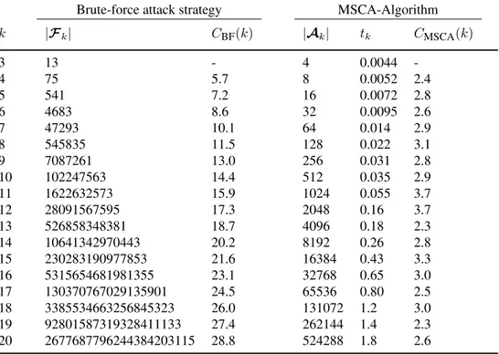
The results of the comparative study are shown in Table2and Figure1. Note that the complexity rate for MCSA-Algorithm remains between[2,4]fork ≤20. However the rate for the brute-force strategy grows linearly. That reveals that our proposal is efficient and competitive.
The reported computation time in Table2corresponds to an average over 100 problems on a Dell Precision T7500. Data management and analysis was per-formed using a equipped with two Intel Xeon X5550 v2 processors - 4 cores, each working at 2.66 GHz - and 24 GB RAM. Matlab and Gurobi optimizer were com-bined to solve the problems. In addition, since RAI-Algorithm allows to generate the A set, the computation of Mahalanobis consensus solution can be trivially parallelized. Therefore the computations time on Table 2 can be reduced using the current generation of calculation platforms.
0 5 10 15 20
0 5 10 15 20 25 30
Number of alternatives(k)
Complexity
rate
Brute-force attack
0 5 10 15 20
0 1 2 3 4 5
Number of alternatives(k)
Complexity
rate
MCSA-Algorithm
Figure 1: Complexity rate for a brute-force attack strategy and for the MSCA-Algorithm versus the number of alternatives (k).
In the coming section the novel procedures and algorithms exposed in this work are put in practice in a real case.
to(1, . . . ,1)due to the fact that the associated feasible set is the biggest and heuristically, the
Brute-force attack strategy MSCA-Algorithm
k |Fk| CBF(k) |Ak| tk CMSCA(k)
3 13 - 4 0.0044
-4 75 5.7 8 0.0052 2.4
5 541 7.2 16 0.0072 2.8
6 4683 8.6 32 0.0095 2.6
7 47293 10.1 64 0.014 2.9
8 545835 11.5 128 0.022 3.1
9 7087261 13.0 256 0.031 2.8
10 102247563 14.4 512 0.035 2.9
11 1622632573 15.9 1024 0.055 3.7
12 28091567595 17.3 2048 0.16 3.7
13 526858348381 18.7 4096 0.18 2.3
14 10641342970443 20.2 8192 0.26 2.8
15 230283190977853 21.6 16384 0.43 3.3
16 5315654681981355 23.1 32768 0.65 3.0
17 130370767029135901 24.5 65536 0.80 2.5
18 3385534663256845323 26.0 131072 1.2 3.0
19 92801587319328411133 27.4 262144 1.4 2.3
20 2677687796244384203115 28.8 524288 1.8 2.6
Table 2: Main features of the two proposed Mahalanobis consensus solution strategies: brute-force attack and MSCA-Algorithm .
4. A real case: The Spanish social consensus family budget
The experimental work presented here provides one of the first investigations into how to compute the family budgets that more consensus conveys among fami-lies and then, to establish household consumption behaviour9. Particularly, the focus of the work is on Spanish Economy and social consensus family budgets are computed based on Spanish data on 2016 household budgets. As mentioned in Introduction, the knowledge of the Spanish household consumption behaviour allows companies and Governments to improve their marketing and public poli-cies. It is hoped that this real study will contribute to a deeper understanding of the methodologies proposed in the previous Sections.
The remaining part of the section proceeds as follows. Firstly, a a brief over-view of the framework and the traditional approach used in Spain to determine the family budgets is introduced. Secondly, the data provided by the Spanish
National Statistics Institute for the households consumption are manipulated to obtain families’ preferences. Subsequently, the canonical codification of the fam-ilies preferences are computed as well as averages group expenditure. Thereupon, different social consensus family budgets are calculated for different Σmatrices to promote the debate. Finally, the aforementioned results are analysed and dis-cussed.
4.1. The Spanish framework and approach
The SpanishNational Statistics Instituteperforms theHousehold Budget Sur-vey(HBS) since 1958. This survey is one of the oldest in Spain and its main goal is to obtain information on the nature and destination of consumption cost, as well as on various characteristics relating to the conditions of household life.
The survey was last reformed in 2006, it is nowadays annual, includes about 24000 dwellings in its sample and provides essential information on the estimates on households consumption expenditure and on updating theConsumer Price In-dex(CPI) weightings.
The HBS classifies expenses using the COICOP (national adaptation of the international classification used by Eurostatfor budget surveys) and it structures them as follows:
• Group 1: Food and non-alcoholic beverages
• Group 2: Alcoholic beverages, tobacco and narcotics
• Group 3: Clothing and footwear
• Group 4: Housing, water, electricity, gas and other fuels
• Group 5: Furniture, household equipment and ordinary expenses for the maintenance of the dwelling
• Group 6: Health
• Group 7: Transport
• Group 8: Communication
• Group 9: Leisure, performances and culture
• Group 11: Restaurants, coffee and hotels
• Group 12: Miscellaneous goods and services
The National Statistics Institute to estimate the characteristics of households uses the following estimator [32]:
b XA=
X
h∈A
Ph·T
P
g∈hRg ·
P
i∈g[chi·
P
j∈iphij] ·
" X
g∈h
Rg·
X
i∈g
[chi·
X
j∈i
xhij]
#
being:
• XbA: Estimate of the total annual household expenditure on a good or service X in geographical area A.
• Ph: Population projection of stratum h, referring to half of the surveying year.
• T: Temporary elevation factor. This factor depends on the reference period of the good or service X.
• chi: Update coefficient. It is a value that depends on the selection and rep-resents its growth from the moment of sample selection until the year of the data in the survey. For the year 2016 this coefficient is equal to 1.
• phij: Population formed by the household members in household j of the sample, sectioni, stratumh.
• xhij: Value of the expenditure on the good or serviceX in household j of the sample, sectioni, stratumh.
• Rg: Non-response correction factor in group g. It is obtained as the quotient between the total number of households of the theoretical sample of this group and the household of the effective sample.
The previousXbAestimator can also be expressed in the next simplified version bycalibrationapproach:
ˆ XA=
X
k∈A
wherekranges over all of the effective sample units in geographical area A. To obtained this final estimator, it is necessary to find a new weightdkenables
ˆ
XAto verify:
i. The estimate based on the sample of a specific feature must match the value of this feature on the population (this value is obtained through an external source).
ii. Fixed a distance function10, the distance betweend
kandwkshould be min-imal.
In recent years, there has been an increasing interest in analysing the afore-mentioned traditional approach and the main challenges faced by many researchers are (see [33] and [34]):
• Selection of the appropriate equivalence scale to adapt the household bud-gets for different sizes and types.
• Consideration of interrelationships among expenditure groups.
• Establishment of index/weights for geographical differences in prices.
• Updating budgets over time.
Although there are several approaches in the specialized literature to overcome these drawbacks, there is no consensus on it. Therefore, in the pages that follow, this research shows how to implement the new methodology and algorithms raised above that improving such drawbacks.
4.2. Our proposal
Following the group decision making problem framework presented in Sec-tion2, the set of agents considered is composed of the households included in the sample selected by the Spanish National Statistics Institute in 2016:22130 house-hold, thenN ={1, . . . ,22130}. Additionally, the set of alternatives is formed by the twelve expenditure groups11 ,X={x
1, x2, . . . , x12},k= 12.
10A truncated linear distance function is traditionally applied and the computations are
per-formed by the CALMAR software (CALibration of MARgins). This specific software is used by many National Statistics Offices on the world like UK, Ireland, France, and so on.
11The structure of the expenditure groups as well as the sample distribution are preserved in
By means of the HBS, the data of the households consumption expenditure is collected and classified according the expenditure groups12. For the purpose of obtaining the households preferences on the expenditure groups, the consump-tion for each household is aggregated for each expenditure group. After aggrega-ting, the results are ordered to grade the groups, obtained a complete preorder Ri ∈ W(X)onXfor each householdi ={1, . . . , n = 22 130}. These complete preorders generate a particular profile:
P = (R1, . . . ,Rn)∈W(X)×. . .×W(X) = W(X)n=22130
whereRirepresents the preferences of the householdion the twelve expenditure groups for eachi= 1, . . . ,22 130.
Applying Definition1 to each complete preorder the codified profile for P,
MP ∈M22 130×12is obtained.
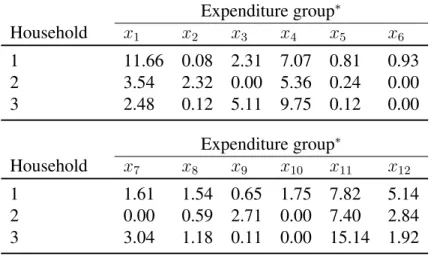
By way of illustration of this first procedure, Table3 shows the expenditure of three families from the sample in the groups of goods. Taking into account the data from Table3, the household preferences are:
• Household 1:
R1 :x2 ≺x9 ≺x5 ≺x6 ≺x8 ≺x7 ≺x10≺x3 ≺x12≺x4 ≺x11 ≺x1
• Household 2:
R2 :x3 ∼x6 ∼x7 ∼x10≺x5 ≺x8 ≺x2 ≺x9 ≺x12≺x1 ≺x4 ≺x11
• Household 3:
R3 :x6 ∼x10≺x9 ≺x5 ≺x2 ≺x8 ≺x12≺x1 ≺x7 ≺x3 ≺x4 ≺x11
12All data available through the website: http://www.ine.es/dyngs/INEbase/en/
Expenditure group∗
Household x1 x2 x3 x4 x5 x6
1 11.66 0.08 2.31 7.07 0.81 0.93
2 3.54 2.32 0.00 5.36 0.24 0.00
3 2.48 0.12 5.11 9.75 0.12 0.00
Expenditure group∗
Household x7 x8 x9 x10 x11 x12
1 1.61 1.54 0.65 1.75 7.82 5.14
2 0.00 0.59 2.71 0.00 7.40 2.84
3 3.04 1.18 0.11 0.00 15.14 1.92
∗: data in thousands of euro.
Table 3: Expenditure for group from original data.
Once the household preferences have been established, the corresponding pre-orders, R1,R2 andR3 are codified following Definition1. Table 4shows these
codified complete preorders:
cRi
Household c1 c2 c3 c4 c5 c6
1 12 1 8 10 3 4
2 10 7 4 11 5 4
3 8 5 10 11 4 2
cRi
Household c7 c8 c9 c10 c11 c12
1 6 5 2 7 11 9
2 4 6 8 4 12 9
3 9 6 3 2 12 7
Table 4: Codified complete preordersRi fori= 1,2,3
1. To compute the average of the canonical codified profile:
mP = (m1, . . . , m12)
The elements ofmP vector are showed in Table5.
2. To fix aΣmatrix. This matrix should convey the specific characteristics of the problem at hand. The role of theΣmatrix allows to take into account the variances of the expenditure groups and the covariances among them. In this contribution, several different Σmatrices were considered to promote the discussion and to capture the interrelations among the twelve expenditure groups:
• Σ1 = Id matrix. The simplest case. The Σ matrix is the identity
matrix, then all expenditure groups are equally treated.
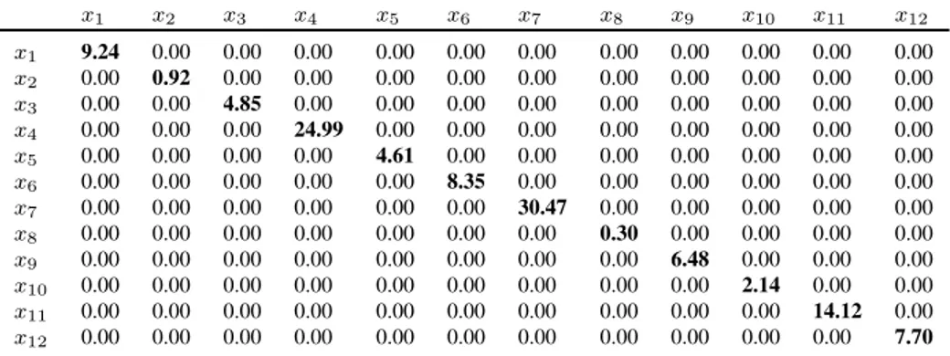
• Σ2 matrix. This Σ matrix accounts the case where the expenditure
groups are considered differently by means of a diagonal matrix. Spe-cifically, Σ2 includes like diagonal elements the variances of the
ex-penditure groups from the original data. Table6includes this particu-lar matrix.
• Σ3 matrix. A natural choice could be to consider the Σ matrix like
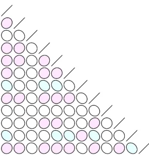
the empirical variance-covariance matrix computed directly from the original data (without codification). This matrix involves not only that all expenditure groups are not equally treated but they are also corre-lated. Figure2presents a graphical interpretation of such relations13. Table7showsΣ3and its corresponding correlation matrix is in Table
8.
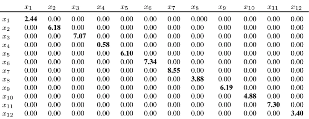
• Σ4 matrix. Similar to Σ2 matrix, Σ4 is a diagonal matrix which
in-cludes like diagonal elements the variances of the expenditure groups but from the codified profile as shows Table9.
• Σ5 matrix. Since the objective function in the optimization problem
uses the Mahalanobis distance among canonical codified preorders, it is reasonable to propose likeΣmatrix the statistical variance-covarince matrix computed from the codified profile. This matrix Σ5 and its
correlation matrix13.
• Σ6 matrix. This special Σ matrix has been designed to capture the
correlations among the group of expenditures from original data and to adapt them to the scale of the codified profile. To this aim, Σ6 is
defined by
Σ6 =D·R·D
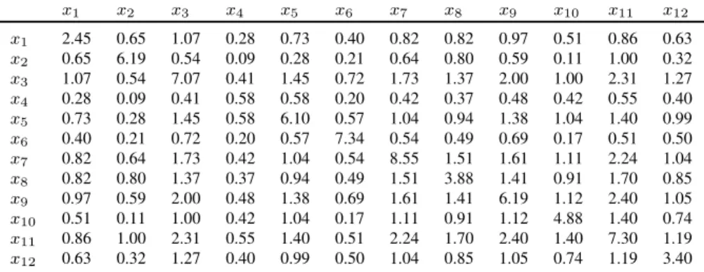
where R is the correlation matrix computed from the twelve expen-diture groups (Table 8) and D the diagonal matrix which diagonal elements are the square roots of the variances of the codified profile (Table10). TheΣ6matrix is showed in Table12.
3. To establish the feasible set. As mentioned in Subsection2.3, the feasible set in this problem is finite, although for k = 12, the number of complete preorders to consider is φ(12) = 28 091 567 595 ≈ 3e + 10 (see [35]). To manage such a number of preorders, Algorithm 1is put in practice, to compute theα-indices setA12(|A12|= 211= 2048).
4. To solve the quadratic optimization problems. For eachα∈A12we solve:
min c∈Fα
dΣm(mP,c)
or in matrix form:
min (mP −c) Σm−1 (mP−c)t
s.a.
Id B1 . . . B12 0 C1 . . . C12 0 Id . . . Id
ct bt
1
.. .
bt
12
=
0t
1t
αt
whereId,{Bi}12i=1,{Ci}12i=1 ∈M12×12and0,1,{bi}12i=1 ∈R12.
Finally, among2048solutions associated to eachFα, we select the codified
preordercthat produces the best agreement.
13Ellipses in Figures 2and3 symbolize the correlation between two expenditure groups.
Algorithm 2 reveals that the social consensus family budgets for the six Σ
matrices are given by:
Σ1: x4 x1 x12x7 x9 x11 x3 ∼x5 x2 ∼x6 ∼x8 ∼x10.
Σ2: x4 x1 x7 x11x12 x9 x3 ∼x8 x2 ∼x5 ∼x6 ∼x10.
Σ3: x4 x1 x7 x11x12 x9 x3 ∼x8 x2 ∼x5 ∼x6 ∼x10.
Σ4: x4 x1 x7 x11x12 x9 x3 ∼x5 ∼x8 x2 ∼x6 ∼x10.
Σ5: x4 x7 x1 x11x12 x9 x8 x3 x5 ∼x2 ∼x6 ∼x10.
Σ6: x4 x1 x7 x12x11 x9 x8 ∼x5 ∼x3 x2 ∼x6 ∼x10.
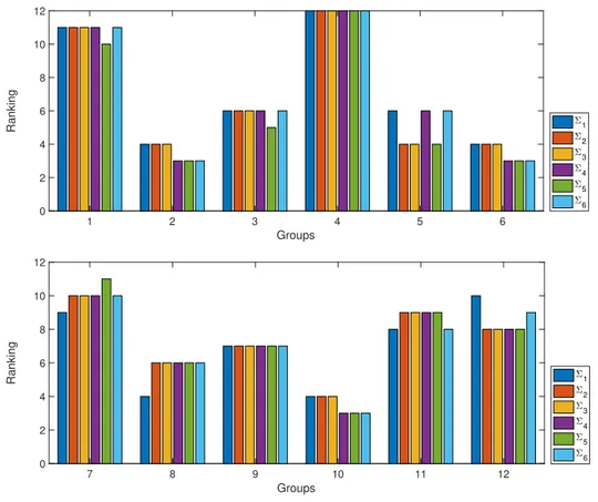
Moreover the group position for differentΣas well as the values of the objec-tive function are displayed in Table13and showed in Figures4and5.
Note that the calculation time employed to obtain the solutions aforemen-tioned on a Dell Precision T7500 (equipped with two Intel Xeon X5550 v2 pro-cessors – 4 cores, each working at 2.66 GHz – and 24 GB RAM) is on the order of 80 seconds. A brute-force procedure should calculate the distance between pre-orders in a time of approximately3.5e+ 8preorders per second to be competitive with the procedure implemented by Algorithms1and2.
4.3. Discussion
The present case of study was designed to analyse consumer behaviour from a non-standard point of view. The results of this study indicate that different social consensus family budgets are obtained if the expenditure groups are not equally treated as well as if the interrelations among them are taken into account.
In reviewing the literature, no data was found on the inclusion of such re-lationships in the traditional computation on the family budgets. This fact may disturb the results of the analyses of the consumer behaviour obtained and also the computation of the consumer price index (CPI).
Closer inspection of the outcomes obtained in Subsection4.2 and Figures4 and5, reveals thatx4the expenditure group 4 (Housing, water, electricity, gas and
other fuels), appears on the top of the social consensus family budget for eachΣ
matrix.
The solutions obtained forΣ2andΣ3coincide among them althoughΣ3takes
magnitude of the original data, that is, the large figures included in theΣmatrix skew the preorders included in the codified profile and then the results. This prob-lem is solved by including the special matrix,Σ6. This particular matrix has been
built to adapt the correlations among the original data from expenditure groups to the scale of the codified profile.
For Σ4 and Σ5 the solutions obtained are similar but not equal. To be
pre-cise, forΣ5the social solution presents less expenditure groups indifferent among
them, for instance: x8 x3 x5 for Σ5 against x8 ∼ x3 ∼ x5 for Σ3, due
to the incorporation of the interrelation among them even if their correlations are relatively small (see Tables10,11and Figures3,4and5).
About the change of expenditure group position respect toΣi, note that groups
x7 (transport) andx12(services) are the more affected. Whereas the solution for
Σ1 ordersx7 in the2nd position, the choiceΣ5 sets this group at4th position. A
similar situation is presented for the alternativex12(see Figure5). It reveals that
the correlations among expenditure groups affects the final ranking of alternatives.
Together these results provide important insights into the relevance of con-sidering the relationship among expenditure groups and the data scale in order to compute the consumers’ behaviour (goods ranking) that more consensus conveys to the society. Hence, it could conceivably be hypothesised that the Σ6 matrix
provides the best solution:
x4 x1 x7 x12 x11 x9 x8 ∼x5 ∼x3 x2 ∼x6 ∼x10
5. Conclusions and futher research work
α-index algorithm (RAI), to establish the feasible set and an algorithm to compute Mahalanobis consensus solutions, the Mahalanobis consensus solution algorithm (MCSA).
Finally and in order to show the several practical applications of this research, a new approach is proposed to analyse consumers’ behaviour. The empirical find-ings in this study provide a new understanding of computing family budgets, the consensus family budgets. Based on Spanish data on household budgets from 2016, the rankings of the expenditure groups that best agrees with family preferen-ces are obtained under different assumptions.
Regarding future research, this contribution has thrown up many questions in need further investigation among which the following are noteworthy:
i. The computation of Mahalanobis consensus solutions requires to have a reference matrix suitable to the problem at hand. Therefore, it is essential to develop procedures to determine such a reference matrix. In this sense, it could be interesting to design methodologies for generating this matrix by means of an endogenous way.
ii. Theα-codification proposed in this paper could also be used to generated the feasible setF.
iii. Future studies related to Social Choice Theory and Preference Behaviour Theory could be inspired by this research particularly, decision making problems that have a not small set of alternatives.
Acknowledgements
The authors thank the three anonymous reviewers and Benjamin Lev (Editor-in-Chief) for their valuable comments and recommendations. The authors ac-knowledge financial support by the Spanish Ministerio de Econom´ıa y Competi-tividad under Project ECO2016-77900-P (T. Gonz´alez-Arteaga and R. de Andr´es Calle) and by the Conserjer´ıa de Educaci´on of the Junta de Castilla y Le´on under Project SA020U16 (J.M. Casc´on).
References
[1] N. M. Fraser, Ordinal preference representations, Theory and Decision 36 (1) (1994) 45–67.
[3] F. Chiclana, F. Herrera, E. Herrera-Viedma, Integrating multiplicative pref-erence relations in a multipurpose decision-making model based on fuzzy preference relations, Fuzzy Sets and Systems 122 (2) (2001) 277 – 291.
[4] J. Borda, M´emoire sur les Elections au Scrutin, Histoire de l’Academie Royale des Sciences, Paris, 1781.
[5] M. Kendall, Rank Correlation Methods, Hafner Publishing Company, New York, 1962.
[6] D. Saari, V. Merlin, A geometric examination of Kemeny’s rule, Social Choice and Welfare 17 (2000) 403–438.
[7] T. Meskanen, H. Nurmi, Mathematics and Democracy, Springer Berlin Hei-delberg, 2006, Ch. Distance from consensus: A theme and variations, pp. 117–132.
[8] C. Klamler, The Dodgson ranking and its relation to Kemeny’s method and Slater’s rule, Social Choice and Welfare 23 (1) (2004) 91–102.
[9] C. Klamler, A distance measure for choice functions, Social Choice and Wel-fare 30 (2008) 419–425.
[10] R. de Andr´es Calle, J. Garc´ıa-Lapresta, J. Gonz´alez-Pach´on, Performance appraisal based on distance function methods, European Journal of Opera-tional Research 207 (3) (2010) 1599 – 1607.
[11] J. Gonz´alez-Pach´on, C. Romero, Inferring consensus weights from pairwise comparison matrices without suitable properties, Annals of Operations Re-search 154 (2004) 123 – 132.
[12] J. Gonz´alez-Pach´on, C. Romero, The design of socially optimal decisions in a consensus scenario, Omega 39 (2) (2011) 179 – 185.
[13] S. France, W. Batchelder, Unsupervised consensus analysis for on-line re-view and questionnaire data, Information Sciences 283 (2014) 241 – 257.
[15] Z. Gong, X. Xu, H. Zhang, U. A. Ozturk, E. Herrera-Viedma, C. Xu, The consensus models with interval preference opinions and their economic in-terpretation, Omega 55 (2015) 81 – 90.
[16] H. Zhang, R. Yang, H. Yan, F. Yang, H∞ consensus of event-based
multi-agent systems with switching topology, Information Sciences In Press.
[17] Y. Akiyama, J.N., M. Darrah, M. Rahem, L. Wang, A method for measuring consensus within groups: An index of disagreement via conditional proba-bility, Information Sciences 345 (2016) 116 – 128.
[18] T. Gonz´alez-Arteaga, R. de Andr´es Calle, J. Alcantud, A new consensus ranking approach for correlated ordinal information based on mahalanobis distance, Information Sciences 372 (Supplement C) (2016) 546 – 564.
[19] G. A. Miller, The magical number seven, plus or minus two: some limits on our capacity for processing information, Psychological Review 63 (1956) 81–97.
[20] D. Li, X. Sun, Nonlinear Integer Programming, Springer US, 2006.
[21] I. J. Good, The number of orderings of n candidates when ties are permitted, Fibonacci Quart. 13 (1975) 11 – 18.
[22] R. W. Bailey, The number of weak orderings of a finite set, Social Choice and Welfare 15 (4) (1998) 559–562.
[23] M. Solomon, R. Russell-Bennett, J. Previte, Consumer Behaviour, Pearson Higher Education, 2012.
[24] A. Biswas, M. Roy, Green products: an exploratory study on the consumer behaviour in emerging economies of the East, Journal of Cleaner Production 87 (2015) 463 – 468.
[25] M. M. Wei, F. Zhang, Recent research developments of strategic consumer behavior in operations management, Computers&Operations Research 93 (2018) 166 – 176.
[27] D. Black, Partial justification of the Borda count, Public Choice 28 (1976) 1–16.
[28] W. Cook, L. Seiford, On the Borda–Kendall consensus method for priority ranking problems, Management Science 28 (1982) 621–637.
[29] J. L. Garc´ıa-Lapresta, D. P´erez-Rom´an, Measuring consensus in weak or-ders, in: E. Herrera-Viedma, J. L. Garc´ıa-Lapresta, J. Kacprzyk, M. Fedrizzi, H. Nurmi, S. Zadrozny (Eds.), Consensual Processes, Vol. 267 of Studies in Fuzziness and Soft Computing, Springer Berlin Heidelberg, 2011, pp. 213– 234.
[30] Matlab r2017a, The MathWorks, Inc., Natick, Massachusetts, USA, http://www.mathworks.com.
[31] Gurobi optimizer, v7, Houston, USA. Free Academic License, http://www.gurobi.com.
[32] Household budget survey. Methodology, INE,
http://www.ine.es/dyngs/INEbase.
[33] H. Watts, Special panel suggests changes in bls family budget program, Monthly Labor Review 103 (12) (1980) 3–10.
[34] D. Johnson, T. Garner, Developing poverty thresholds using expenditure data, in: Proceedings of the Government and Social Statistics Section, 1997, pp. 28–37.
Group
x1 x2 x3 x4 x5 x6
Average Expenditure∗ 4.47 0.55 1.5 9.03 1.23 1.05
mi 10.08 4.22 6.06 11.61 5.71 4.78
Group
x7 x8 x9 x10 x11 x12
Average Expenditure∗ 3.31 0.82 1.69 0.41 2.68 2.15
mi 7.51 5.7 6.39 3.14 7.43 7.9
∗: data in thousands of euro.
Table 5: Expenditure averages for original data and codified data.
x1 x2 x3 x4 x5 x6 x7 x8 x9 x10 x11 x12
x1 9.24 0.00 0.00 0.00 0.00 0.00 0.00 0.00 0.00 0.00 0.00 0.00
x2 0.00 0.92 0.00 0.00 0.00 0.00 0.00 0.00 0.00 0.00 0.00 0.00
x3 0.00 0.00 4.85 0.00 0.00 0.00 0.00 0.00 0.00 0.00 0.00 0.00
x4 0.00 0.00 0.00 24.99 0.00 0.00 0.00 0.00 0.00 0.00 0.00 0.00
x5 0.00 0.00 0.00 0.00 4.61 0.00 0.00 0.00 0.00 0.00 0.00 0.00
x6 0.00 0.00 0.00 0.00 0.00 8.35 0.00 0.00 0.00 0.00 0.00 0.00
x7 0.00 0.00 0.00 0.00 0.00 0.00 30.47 0.00 0.00 0.00 0.00 0.00
x8 0.00 0.00 0.00 0.00 0.00 0.00 0.00 0.30 0.00 0.00 0.00 0.00
x9 0.00 0.00 0.00 0.00 0.00 0.00 0.00 0.00 6.48 0.00 0.00 0.00
x10 0.00 0.00 0.00 0.00 0.00 0.00 0.00 0.00 0.00 2.14 0.00 0.00
x11 0.00 0.00 0.00 0.00 0.00 0.00 0.00 0.00 0.00 0.00 14.12 0.00
x12 0.00 0.00 0.00 0.00 0.00 0.00 0.00 0.00 0.00 0.00 0.00 7.70
x1 x2 x3 x4 x5 x6 x7 x8 x9 x10 x11 x12
x1 9.24 0.48 1.71 3.54 1.23 0.83 3.01 0.44 1.92 0.65 2.33 1.83
x2 0.48 0.92 0.17 0.21 0.09 0.08 0.46 0.08 0.23 0.02 0.53 0.18
x3 1.71 0.17 4.85 2.20 1.04 0.63 2.70 0.31 1.69 0.55 2.65 1.58
x4 3.54 0.21 2.20 24.99 3.31 1.42 5.16 0.67 3.23 1.84 4.99 3.99
x5 1.23 0.09 1.04 3.31 4.60 0.53 1.70 0.22 1.22 0.60 1.68 1.29
x6 0.83 0.08 0.63 1.42 0.53 8.35 1.09 0.14 0.74 0.11 0.75 0.80
x7 3.01 0.46 2.70 5.16 1.70 1.09 30.47 0.79 3.10 1.38 5.88 2.94
x8 0.44 0.08 0.31 0.67 0.22 0.14 0.79 0.30 0.40 0.16 0.66 0.35
x9 1.92 0.23 1.69 3.23 1.22 0.74 3.10 0.40 6.48 0.75 3.41 1.61
x10 0.65 0.02 0.55 1.84 0.60 0.11 1.38 0.16 0.75 2.14 1.29 0.73
x11 2.33 0.53 2.65 4.99 1.68 0.75 5.88 0.66 3.41 1.29 14.12 2.48
x12 1.83 0.18 1.58 3.99 1.29 0.80 2.94 0.35 1.61 0.73 2.48 7.70
∗
: data in thousands of euro.
Table 7: Σ3: Variance-Covariance matrix of the expenditure groups from original
data.
x1 x2 x3 x4 x5 x6 x7 x8 x9 x10 x11 x12
x1 1.00 0.17 0.26 0.23 0.19 0.09 0.18 0.26 0.25 0.15 0.20 0.22
x2 0.17 1.00 0.08 0.05 0.05 0.03 0.09 0.16 0.09 0.02 0.15 0.07
x3 0.26 0.08 1.00 0.20 0.22 0.10 0.22 0.26 0.30 0.17 0.32 0.26
x4 0.23 0.05 0.20 1.00 0.31 0.10 0.19 0.24 0.25 0.25 0.27 0.29
x5 0.19 0.05 0.22 0.31 1.00 0.09 0.14 0.19 0.22 0.19 0.21 0.22
x6 0.09 0.03 0.10 0.10 0.09 1.00 0.07 0.09 0.10 0.03 0.07 0.10
x7 0.18 0.09 0.22 0.19 0.14 0.07 1.00 0.26 0.22 0.17 0.28 0.19
x8 0.26 0.16 0.26 0.24 0.19 0.09 0.26 1.00 0.29 0.21 0.32 0.23
x9 0.25 0.09 0.30 0.25 0.22 0.10 0.22 0.29 1.00 0.20 0.36 0.23
x10 0.15 0.02 0.17 0.25 0.19 0.03 0.17 0.21 0.20 1.00 0.24 0.18
x11 0.20 0.15 0.32 0.27 0.21 0.07 0.28 0.32 0.36 0.24 1.00 0.24
x12 0.22 0.07 0.26 0.29 0.22 0.10 0.19 0.23 0.23 0.18 0.24 1.00
Table 8: Correlation matrix computed from original data.
x1 x2 x3 x4 x5 x6 x7 x8 x9 x10 x11 x12
x1 2.44 0.00 0.00 0.00 0.00 0.00 0.00 0.000 0.00 0.00 0.00 0.00
x2 0.00 6.18 0.00 0.00 0.00 0.00 0.00 0.00 0.00 0.00 0.00 0.00
x3 0.00 0.00 7.07 0.00 0.00 0.00 0.00 0.00 0.00 0.00 0.00 0.00
x4 0.00 0.00 0.00 0.58 0.00 0.00 0.00 0.00 0.00 0.00 0.00 0.00
x5 0.00 0.00 0.00 0.00 6.10 0.00 0.00 0.00 0.00 0.00 0.00 0.00
x6 0.00 0.00 0.00 0.00 0.00 7.34 0.00 0.00 0.00 0.00 0.00 0.00
x7 0.00 0.00 0.00 0.00 0.00 0.00 8.55 0.00 0.00 0.00 0.00 0.00
x8 0.00 0.00 0.00 0.00 0.00 0.00 0.00 3.88 0.00 0.00 0.00 0.00
x9 0.00 0.00 0.00 0.00 0.00 0.00 0.00 0.00 6.19 0.00 0.00 0.00
x10 0.00 0.00 0.00 0.00 0.00 0.00 0.00 0.00 0.00 4.88 0.00 0.00
x11 0.00 0.00 0.00 0.00 0.00 0.00 0.00 0.00 0.00 0.00 7.30 0.00
x12 0.00 0.00 0.00 0.00 0.00 0.00 0.00 0.00 0.00 0.00 0.00 3.40
x1 x2 x3 x4 x5 x6 x7 x8 x9 x10 x11 x12
x1 2.44 0.49 -0.34 0.03 0.14 0.08 -0.97 0.50 -0.426 -0.09 -1.15 0.16
x2 0.49 6.18 -0.95 0.12 0.13 -0.13 -0.86 0.93 -0.81 -0.03 -0.74 0.00
x3 -0.34 -0.95 7.07 -0.13 -0.39 -0.61 -1.03 -0.64 -0.61 -0.17 -0.66 -0.34
x4 0.03 0.12 -0.13 0.58 0.11 0.03 -0.49 0.27 -0.07 0.13 -0.23 0.13
x5 0.14 0.13 -0.39 0.11 6.10 0.36 -1.65 0.35 -0.59 0.36 -1.52 0.39
x6 0.08 -0.13 -0.61 0.03 0.36 7.34 -1.49 0.37 -0.92 -0.01 -1.69 0.22
x7 -0.97 -0.86 -1.04 -0.49 -1.65 -1.49 8.55 -0.95 -0.82 -0.48 0.17 -1.07
x8 0.50 0.93 -0.64 0.27 0.35 0.37 -0.95 3.88 -0.58 0.61 -1.27 0.67
x9 -0.42 -0.81 -0.61 -0.07 -0.59 -0.92 -0.82 -0.58 6.19 -0.03 -0.12 -0.66
x10 -0.09 -0.03 -0.17 0.13 0.36 -0.01 -0.48 0.61 -0.03 4.88 -0.32 0.15
x11 -1.15 -0.74 -0.66 -0.23 -1.52 -1.69 0.16 -1.27 -0.12 -0.32 7.30 -1.14
x12 0.16 0.00 -0.35 0.13 0.39 0.23 -1.07 0.67 -0.65 0.15 -1.14 3.39
Table 10: Σ5: Variance-Covariance matrix computed of the codified profile.
x1 x2 x3 x4 x5 x6 x7 x8 x9 x10 x11 x12
x1 1.00 0.13 -0.08 0.03 0.04 0.02 -0.21 0.16 -0.11 -0.03 -0.27 0.06
x2 0.13 1.00 -0.14 0.06 0.02 -0.02 -0.12 0.19 -0.13 -0.01 -0.11 0.00
x3 -0.08 -0.14 1.00 -0.07 -0.06 -0.08 -0.13 -0.12 -0.09 -0.03 -0.09 -0.07
x4 0.03 0.06 -0.07 1.00 0.06 0.02 -0.22 0.18 -0.04 0.08 -0.12 0.10
x5 0.04 0.02 -0.06 0.06 1.00 0.05 -0.23 0.07 -0.10 0.07 -0.23 0.09
x6 0.02 -0.02 -0.08 0.02 0.05 1.00 -0.19 0.07 -0.14 -0.00 -0.23 0.05
x7 -0.21 -0.12 -0.13 -0.22 -0.23 -0.19 1.00 -0.16 -0.11 -0.07 0.02 -0.20
x8 0.16 0.19 -0.12 0.18 0.07 0.07 -0.16 1.00 -0.12 0.14 -0.24 0.19
x9 -0.11 -0.13 -0.09 -0.04 -0.10 -0.14 -0.11 -0.12 1.00 -0.01 -0.02 -0.14
x10 -0.03 -0.01 -0.03 0.08 0.07 -0.00 -0.07 0.14 -0.01 1.00 -0.05 0.04
x11 -0.27 -0.11 -0.09 -0.12 -0.23 -0.23 0.02 -0.24 -0.02 -0.05 1.00 -0.23
x12 0.06 0.00 -0.07 0.10 0.09 0.05 -0.20 0.19 -0.14 0.04 -0.23 1.00
Table 11: Correlation matrix from the codified profileMP.
x1 x2 x3 x4 x5 x6 x7 x8 x9 x10 x11 x12
x1 2.45 0.65 1.07 0.28 0.73 0.40 0.82 0.82 0.97 0.51 0.86 0.63
x2 0.65 6.19 0.54 0.09 0.28 0.21 0.64 0.80 0.59 0.11 1.00 0.32
x3 1.07 0.54 7.07 0.41 1.45 0.72 1.73 1.37 2.00 1.00 2.31 1.27
x4 0.28 0.09 0.41 0.58 0.58 0.20 0.42 0.37 0.48 0.42 0.55 0.40
x5 0.73 0.28 1.45 0.58 6.10 0.57 1.04 0.94 1.38 1.04 1.40 0.99
x6 0.40 0.21 0.72 0.20 0.57 7.34 0.54 0.49 0.69 0.17 0.51 0.50
x7 0.82 0.64 1.73 0.42 1.04 0.54 8.55 1.51 1.61 1.11 2.24 1.04
x8 0.82 0.80 1.37 0.37 0.94 0.49 1.51 3.88 1.41 0.91 1.70 0.85
x9 0.97 0.59 2.00 0.48 1.38 0.69 1.61 1.41 6.19 1.12 2.40 1.05
x10 0.51 0.11 1.00 0.42 1.04 0.17 1.11 0.91 1.12 4.88 1.40 0.74
x11 0.86 1.00 2.31 0.55 1.40 0.51 2.24 1.70 2.40 1.40 7.30 1.19
x12 0.63 0.32 1.27 0.40 0.99 0.50 1.04 0.85 1.05 0.74 1.19 3.40
Table 12: Σ6. This matrix contains the covariances computed from the gadget and
Correlations calculated with expenditures
group.1
group.2
group.3
group.4
group.5
group.6
group.7
group.8
group.9
group.10
group.11
group.12
group
.1
group
.2
group
.3
group
.4
group
.5
group
.6
group
.7
group
.8
group
.9
group
.10
group
.11
group
.12
Figure 2: Graphical interpretation of the correlation matrix (Table8) of the Spa-nish expenditure groups from original data.
Group
O. F. value x1 x2 x3 x4 x5 x6 x7 x8 x9 x10 x11 x12
Σ1 12.64 11 4 6 12 6 4 9 4 7 4 8 10
Σ2 1.9 11 4 6 12 4 4 10 6 7 4 9 8
Σ3 2.04 11 4 6 12 4 4 10 6 7 4 9 8
Σ4 2.43 11 3 6 12 6 3 10 6 7 3 9 8
Σ5 3.5 10 3 5 12 4 3 11 6 7 3 9 8
Σ6 2.41 11 3 6 12 6 3 10 6 7 3 8 9
Correlations calculated with codified profiles group.1 group.2 group.3 group.4 group.5 group.6 group.7 group.8 group.9 group.10 group.11 group.12 group .1 group .2 group .3 group .4 group .5 group .6 group .7 group .8 group .9 group .10 group .11 group .12
Figure 3: Graphical interpretation of the correlation matrix (Table11) of the Spa-nish expenditure groups from codified profile.
1 2 3 4 5 6
matrices 0 2 4 6 8 10 12 Ranking Group.1 Group.2 Group.3 Group.4 Group.5 Group.6 Group.7 Group.8 Group.9 Group.10 Group.11 Group.12
Figure 4: Group position/ranking for{Σi}6i=1 matrices. Results are clustered
1 2 3 4 5 6
Groups
0 2 4 6 8 10 12
Ranking 1
2 3 4 5 6
7 8 9 10 11 12
Groups
0 2 4 6 8 10 12
Ranking 1
2 3 4 5 6
Figure 5: Group position/ranking for {Σi}6i=1 matrices. Results are clustered by