Local quantum measurement discrimination

Texto completo

(1)PHYSICAL REVIEW A 75, 012107 共2007兲. Local quantum measurement discrimination D. Mundarain1 and M. Orszag2. 1. Departments de Física, Universidad Simon Bolívar, Apartado Postal 89000, Caracas 1080A, Venezuela 2 Facultad de Física, Pontificia Universidad Católica de Chile, Casilla 306, Santiago, Chile 共Received 9 November 2006; published 12 January 2007兲. We study a scheme for a local quantum measurement discrimination, i.e., the estimation via local measurements on B of previous measurements done in A for a composed bipartite system AB. The common bath plays a crucial role in the process. DOI: 10.1103/PhysRevA.75.012107. PACS number共s兲: 03.65.Ud, 03.65.Ta. I. INTRODUCTION. In 1982 Herbert presented his famous paper “Flash—A superluminal communicator based upon a new kind a measurement” 关1兴. In his paper this author presented a clever scheme of measurements that allowed, by doing a local measurements on system B, to infer what observable was previously measured in a system A, for a bipartite entangled system AB. As everybody knows, his proposal was wrong since it violated the no-cloning theorem, which was proved later 关2,3兴. In a beautiful note presented in the Los Alamos National Laboratory 共LANL兲 archives 关4兴, Peres considered “what kind of modifications of quantum mechanics would allow the information transfer by means of local quantum operations 共LQO兲.” He argued that relaxing the linearity condition of quantum mechanics it is possible to obtain a local quantum measurement discrimination: after the measurement in A, a nonlinear local evolution of B yields different mixed states of B for different measurements of observables in A. These states can be distinguished statistically. Unfortunately, since quantum mechanics is linear, it seems that there could be no local measurement in B that would be able to discriminate what Alice was measuring. The Peres proposal considers only LQO, and also the individual evolution of B after the measurement in A. In this work we are going to relax this restriction and consider a global evolution between the two local measurements. It seems obvious that if there exist some kind of information flow between the two subsystems after the measurement in A and before the measurement in B, the discrimination would be possible. The global evolution can generate this flow of information, and the reduced dynamics of a given subsystem will be nonlinear, thus allowing the local quantum discrimination. We are going to consider a system of two particles with two quantum levels in the presence of a common squeezed bath. In this case the quantum global evolution of the composed system is described in terms of a master equation. We are going to show that this configuration will allow the discrimination between measurements of two given observables, initially performed on A, by local measurement on B over the stationary states of the system. The structure of the work is the following one: Section II shows why the local measurements do not allow the discrimination. In Sec. III we review the dynamics of two two-level systems in a common squeezed bath, particularly paying attention to the stationary 1050-2947/2007/75共1兲/012107共5兲. states of the system. Section IV considers the first type of problem: by performing local measurements on B one can determine if the observable ␴zA was previously measured or not. In Sec. V we consider the second type: a local discrimination of two observables. Finally, in Sec. VI we discuss the results and present some conclusions. II. LOCAL MEASUREMENTS. Consider two observers, Alice and Bob, who have a bipartite quantum system described by a known state ␳. They can do local measurements on the subsystems A and B, respectively. If Alice does some measurements on A and Bob does not know the results of those measurements, the reduced state of system B is. ␳B = TrA兵⌺iAi␳A†i 其,. 共1兲. where Ai are the “detector operators” associated to the elements of a POVM 共positive operator valued measurement兲 ␲i = A†i Ai satisfying the usual condition ⌺iA†i Ai = 1. Now Bob performs a local measurement on B. The mean value of any observable ⌸B is 具⌸B典 = TrAB兵⌺iAi␳A†i ⌸B其 = TrA兵⌺iAi TrB兵␳⌸B其A†i 其 = TrA兵⌺iA†i Ai TrB兵␳⌸B其其 = TrB兵TrA兵␳其⌸B其.. 共2兲. In particular if the observable 共⌸B兲 is a projector then this mean value is the probability for some particular result of the local measurement in B 关4兴. Since the result of Eq. 共2兲 does not depend on the Ai operators, Bob cannot decide what measurements Alice did, or worse, he cannot even tell if she had measured or not, without her help. III. TWO TWO-LEVEL SYSTEMS IN A COMMON SQUEEZED BATH. In the interaction picture the master equation for two twolevel systems in a broadband squeezed vacuum has the following structure 关5,7兴:. 012107-1. ⳵␳ ␥ = 兵2S␳S† − ␳S†S − S†S␳其, ⳵t 2. 共3兲. ©2007 The American Physical Society.

(2) PHYSICAL REVIEW A 75, 012107 共2007兲. D. MUNDARAIN AND M. ORSZAG. where. ␣=. S = 冑N + 1⌺ − 冑N exp兵i␺其⌺† = cosh共r兲⌺ − sinh共r兲exp兵i␺其⌺† . 共4兲. ⌺ = ␴ A + ␴ B,. ⌺ =. ␴A†. +. ␴B† ,. 兩␭±典AB =. 冑. 兩␺1典 = 兩␭+典A 丢兩␭−典B ,. 共6兲. 兩␺2典 = 兩␭−典A 丢兩␭+典B ,. 共7兲. N 兩 + 典AB ⫿ i N+M. 冑. M −i␺/2 e 兩− 典AB . N+M. 共8兲. 1. 兩␾2典 = D共兩␺1典 − 兩␺2典兲 =. ␳S =. 1. 共10兲. where C and D are normalization constants and we have used the notation 兩 ± , ± 典 = 兩 ± 典A 丢兩 ± 典B and 兩 ± , ⫿ 典 = 兩 ± 典A 丢兩 ⫿ 典 B. Now, one can construct the basis of the four-dimensional Hilbert space of the two particles incorporating the following two orthogonal vectors: 兩 ␾ 3典 =. 1. 冑2 共兩− , + 典 + 兩 + ,− 典兲,. 冢. 1 − ␳22共0兲 ␳12共0兲 0 0. ␳21共0兲 0 0. ␳22共0兲 0 0 0 0 0 0 0 0. 冣. .. 共17兲. It is important to notice that the stationary states depend on the initial states via the ␳22共0兲 and ␳12共0兲 factors. States with different ␳22共0兲 or ␳12共0兲 provide different stationary states. IV. NO MEASUREMENTS VS MEASUREMENT DISCRIMINATION. 共9兲. 冑2 共兩− , + 典 − 兩 + ,− 典兲,. 共16兲. Consider now the bipartite system initially in the entangled state 兩␾2典,. 冑N2 + M 2 ,. 共N兩 + , + 典 + Me−i␺兩− ,− 典兲,. 共15兲. In this basis the master equation becomes a system of 15 differential equations. The various components of the system are either constant or exponentially decaying terms with rates that depend on ␣, ␤, and ␦. The exponentially decaying terms go to zero and eventually one finds the following stationary state for the master equation:. These two nonorthogonal states allow us to find a basis for the DFS, 兩␾1典 = C共兩␺1典 + 兩␺2典兲 =. 共14兲. 2 . ␣. ␦=. 共5兲. where the subscripts A, B refer to the observables measured by Alice and Bob, respectively. The quantum dynamical semigroup defined by Eq. 共3兲 has an invariant subspace, the decoherence free subspace 共DFS兲: it is the set of all states which are not affected by the squeezed bath. In our particular case the DFS is two dimensional and the following two independent states belong to it 关6兴,. where. 2 , 2N + 1. ␤ = − 2冑N共N + 1兲␣ ,. ␥ is the vacuum decay constant and N , M = 冑N共N + 1兲 and ␺ are the squeeze parameters of the bath. The ⌺ operators are the combined ladder operators for the two particles, †. 冑. 共11兲. 兩⌿共0兲典AB = 兩␾2典 =. 1. 冑2 共兩− , + 典 − 兩 + ,− 典兲.. 共18兲. This state belongs to the DFS and it does not evolve at all in the presence of the common squeezed bath. If Alice does not measure any observable the state remains invariant during the evolution. In that case, when Bob measures ␴ZB the mean value of that observable will be zero at all times. If Alice measures ␴ZB, the total state of system after the measurement becomes. ␳共Z兲共0兲 = 21 兩 + − 典具+ − 兩 + 21 兩− + 典具− + 兩.. 共19兲. In the ⌽ basis this state has a simple matrix representation. 冢冣 0 0 0 0. 兩 ␾ 4典 =. 1. 冑N2 + M 2 共M兩 + , + 典 − Ne. −i␺. 兩− ,− 典兲.. 共12兲. In the basis ⌽ = 兵兩␾1典 , 兩␾2典 , 兩␾3典 , 兩␾4典其 the Lindblad operator S for the two particles has a very simple form. S=. 冢. 0 0 ␣e−i␺ 0 0 0. 0 0 −i␺. 0 0. 0. ␦e. 0 0. ␤. 0. 冣. ,. ␳共Z兲共0兲 =. 1 2. 0. 0 0. 0 0 1 2. 0. ,. 共20兲. 0 0 0 0. which has the following stationary state 关see Eq. 共17兲兴:. 共13兲. ␳共Z兲 S =. 冢冣 1 2. 0 0 0. 0. 1 2. 0 0. 0 0 0 0. 0 0 0 0. where 012107-2. .. 共21兲.

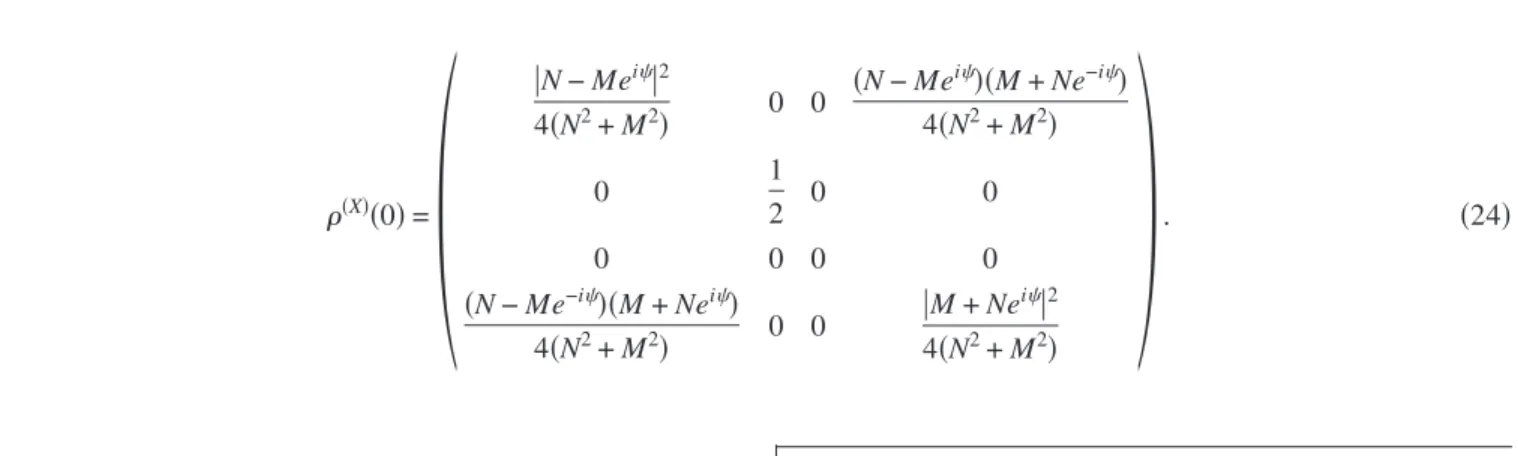
(3) PHYSICAL REVIEW A 75, 012107 共2007兲. LOCAL QUANTUM MEASUREMENT DISCRIMINATION. If Bob performs a measurement on ␴zB long after Alice did hers, i.e., over the stationary state, he obtains the following nonzero mean value: 1 1 N2 − M 2 . 具␴zB典s = 具␾1兩␴zB兩␾1兩典 + 具␾2兩␴zB兩␾2兩典 = 2 2 2共N2 + M 2兲共22兲 In Fig. 1 one can see the evolution of the mean value of ␴zB when Alice does not measure and when she does. Bob can do the discrimination without Alice’s help by simply observing the stationary mean value of ␴zB, if it is zero or different from zero implies that Alice did not or did measure ␴zA, respectively.. 共X兲. ␳ 共0兲 =. 冢. V. LOCAL DISCRIMINATION OF TWO OBSERVABLES. Now we will consider the local discrimination of measurements of two different observables. We assume again that the initial state of the composed system is 兩␾2典. If Alice measures ␴zA, the state after the measurement is given by Eqs. 共19兲 and 共20兲. On the contrary, if Alice measures ␴Ax the state after the measurement becomes. ␳共X兲共0兲 = 41 兵兩 + + 典具+ + 兩 − 兩 + + 典具− − 兩 + 兩 + − 典具+ − 兩 − 兩 + − 典 ⫻具− + 兩 − 兩− + 典具+ − 兩 + 兩− + 典具− + 兩 − 兩− − 典具+ + 兩 + 兩− − 典具− − 兩其.. In the ⌽ basis this state has the following matrix representation:. 兩N − Mei␺兩2 4共N2 + M 2兲. 0 0. 共N − Mei␺兲共M + Ne−i␺兲 4共N2 + M 2兲. 0. 1 0 2. 0. 0. 0 0. 0 兩M + Nei␺兩2 4共N2 + M 2兲. 共N − Me−i␺兲共M + Nei␺兲 0 0 4共N2 + M 2兲. One can observe from Eqs. 共17兲, 共20兲, and 共24兲, that these two different measurements 共␴zA vs ␴Ax 兲 produce the same stationary state at the end of the evolution. However the time evolutions differ. In Fig. 2 we show the evolution of 具␴zB典 for the two measurements when ␺ = 0. In Fig. 3 we show the same quantity for ␺ = ␲. If one considers mean values of ␴zB at finite time it is possible to discriminate the initial measure-. 共23兲. 冣. 共24兲. .. ment. In particular for ␺ = ␲ the discrimination becomes more evident. It is also possible to discriminate the two observables in the stationary state regime. In order to do that, one must take a different initial state: 兩⌿共0兲典AB = 兩␺1典 = 兩␭+典A 丢兩␭−典B .. 共25兲. If Alice measures ␴zA the state after measurements is. 0.2 Alice does not measure Alice measures σz A stationary value <σz B>s. 0.1. 0.1. 0. -0.1. <σz B>(t). <σz B>(t). 0. Alice measures σz A Alice measures σx A. -0.2 -0.3. -0.1. -0.2. -0.4. -0.3. -0.5 -0.6 0. 2. 4. 6. 8. 10. -0.4. γ t. 0. FIG. 1. 具␴zB典共t兲 when Alice does not measure 共solid line兲, Alice measures ␴zA 共line with hollow squares兲. N = 0.1, ␺ = 0. We also show the stationary value 具␴zB典s 共dashed line兲.. 1. 2. 3. 4. 5. γ t. FIG. 2. 具␴zB典共t兲 when Alice measures ␴zA 共solid line兲, Alice measures ␴Ax 共dashed line兲. N = 0.5, ␺ = 0. The initial state is 兩␾2典.. 012107-3.

(4) PHYSICAL REVIEW A 75, 012107 共2007兲. D. MUNDARAIN AND M. ORSZAG. ␳共Z兲共0兲 =. 冉. 冊. N M 兩 + 典AA具+ 兩 + 兩− 典AA具− 兩丢兩␭−典BB具␭−兩. N+M N+M. 共26兲. In the ⌽ basis this state has the following structure:. 共Z兲. ␳ 共0兲 =. 冢. iei␺/2冑NM共N2 + M 2兲. N4 + M 4 共N2 + M 2兲共N + M兲2 − ie. −i␺/2. 冑NM共N. 2. 冑2共N + M兲. +M 兲 2. 冑2共N + M兲 −i␺/2冑 NM共N − M兲 ie 冑2共N + M兲冑N2 + M 2 2. − iei␺/2冑NM共N − M兲. 冑2共N + M兲冑N. 2. 2. NM 共N + M兲2. 0. 0. NM 共N + M兲2. 共N − M兲NM 共N + M兲共N2 + M 2兲. +M. 共N − M兲NM 共N + M兲共N2 + M 2兲. 2. 0 i冑2e−i␺/2冑NM共N − M兲共N + M兲2冑N2 + M 2. − i冑2ei␺/2冑NM共N − M兲. 0. 2N2M 2 共N + M兲2共N2 + M 2兲. 共N + M兲2冑N2 + M 2. and the stationary state associated to this initial state is. ␳共Z兲 S =. 冢. iei␺/2冑NM共N2 + M 2兲. NM 共N + M兲2. 冑2共N + M兲2. 0 0. 冑2共N + M兲2. NM 共N + M兲2. 0 0. 0. 0. 0 0. 0. 0. 0 0. 1−. − ie−i␺/2冑NM共N2 + M 2兲. After some algebra one can obtain the stationary mean value of ␴zB, 具␴zB典共Z兲 S. 共N + M兲共N2 + NM + M 2兲 . = 共N − M兲共N2 + M 2兲. 冋. 1 3共N2 − M 2兲 4共N + M 2兲. 冉冊册. NM共N − M兲 ␺ sin2 N+M 2. 共30兲. .. In Fig. 4 we show the difference between these two mean values for ␺ = 0 and in Fig. 5 the analogous results for ␺ = ␲. As in the previous cases, the discrimination with ␺ = ␲ is a better choice. -0.5. Alice measures σz A Alice measures σx A. 0. Alice measures σz A Alice measures σx A. -0.55. -0.1. <σz B>(t). <σz B>(t). 共27兲. 共28兲. .. 2. −4. 共29兲. We find similar results when Alice measures initially ␴Ax . In this case, after a rather long calculation, we obtain 0.1. 具␴zB典共X兲 S =. 冣. 冣. ,. -0.2. -0.6. -0.65. -0.3 -0.7. -0.4 0. 1. 2. 3. 4. 5. 0. γ t. 2. 4. 6. 8. 10. γ t. FIG. 3. 具␴zB典共t兲 when Alice measures ␴zA 共solid line兲, Alice measures ␴Ax 共dashed line兲. N = 0.5, ␺ = ␲. The initial state is 兩␾2典.. FIG. 4. 具␴zB典共t兲 when Alice measures ␴zA 共solid line兲, Alice measures ␴Ax 共dashed line兲. N = 0.1, ␺ = 0. The initial state is 兩␺1典.. 012107-4.

(5) PHYSICAL REVIEW A 75, 012107 共2007兲. LOCAL QUANTUM MEASUREMENT DISCRIMINATION -0.4. Alice measures σz A Alice measures σx A. -0.45. <σz B>(t). -0.5 -0.55 -0.6 -0.65 -0.7 0. 2. 4. 6. 8. 10. γ t. FIG. 5. 具␴zB典共t兲 when Alice measures ␴zA 共solid line兲, Alice measures ␴Ax 共dashed line兲. N = 0.1, ␺ = ␲. The initial state is 兩␺1典 VI. CONCLUSIONS. In the present work, we have included a global operation, the evolution of the two particles in a common squeezed bath, in order to allow one part of the system to be able to discriminate previous measurements, via Bob’s local measurements only. Without this global evolution the discrimination is only possible by global measurements. In our case we can interpret the evolution process as a measurement process done by one particle over the other one, thus allowing the. 关1兴 N. Herbert, Found. Phys. 12, 1171 共1982兲. 关2兴 W. K. Wootters and W. H. Zurek, Nature 共London兲 299, 802 共1982兲. 关3兴 D. Dieks, Phys. Lett. 92A, 271 共1982兲.. flow of information between the two subsystems. This fact is the central feature of the present local discrimination. It is also interesting to observe that the squeezed bath is particularly convenient for the present discrimination for several reasons. First, it makes the system phase sensitive and one can find the most convenient phase for the optimal discrimination. Also, if we compare, for example with a thermal bath 共T = 0兲, and taking the singlet state, which is the only decoherence free state in this case, we get curves similar to Fig. 2, without the possibility of optimizing with a phase. Also the best discrimination, like in Figs. 4 and 5 are not possible. Finally, it is important to remark that since we have used a common bath, the two particles must be separated a distance not larger than the correlation length of the bath. Also the two local measurements are separated by a time interval of the order of the decay time of the system. If we call lD and ␶D the decoherence length and time, respectively 共lD = c␶D兲, and ␶ = ␥−1, the decay time of the system, and since ␶D Ⰶ ␶, the information transfer velocity between the atoms during a c␶ typical evolution time is of the order of v = ␶D Ⰶ c. Thus, our scheme is not a proposal of superluminal communication like Herbert’s scheme. ACKNOWLEDGMENTS. One of the authors 共D.M.兲 was supported by Did-Usb Grant No. Gid-30 and by Fonacit Grant No. G-2001000712. One of the authors 共M.O.兲 was supported by Fondecyt Grant No. 1051062 and Nucleo Milenio ICM 共P02-049兲. 关4兴关5兴关6兴关7兴. 012107-5. A. Peres, e-print, quant-ph/0205076. C. W. Gardiner, Phys. Rev. Lett. 56, 1917 共1986兲. D. Mundarain and M. Orszag, e-print, quant-ph/0611090. G. S. Agarwal and R. R. Puri, Phys. Rev. A 41, 3782 共1990兲..

(6)