11
APPLICATION OF MARKOV CHANGE DETECTION
TECHNIQUE FOR DETECTING LANDSAT ETM DERIVED
LAND COVER CHANGE OVER BANTEN BAY
Oleh : Antonius B. Wijanarto1
ABSTRACT
Change detection is one of multi temporal analysis in remote sensing that is important for studying the dynamics of environment. Change detection is useful in many applications such as land use changes, habitat fragmentation, rate of deforestation, coastal change, urban sprawl, and other cumulative changes through spatial and temporal analysis techniques such as GIS and Remote Sensing along with digital image processing technique. Markov Change Detection is one application of change detection that can be used to predict future changes based on the rates of past change. The method is based on probability that a given piece of land will change from one mutually exclusive state to another. These probabilities are generated from past changes and then applied to predict future change.
Key words: Change detection, Markov, GIS, Trend analysis
INTRODUCTION
Change detection is a task to compare two sets of imagery to identify changes. The use of satellite data enables change detection to be done over broad spatial scales. This is important, especially when ground measurement of specific map is done rarely. A sensor system used should
have systematic orbital period,
record imagery at the same geographic location and time of the day, maintain the same scale and look angle geometry,
reduce relief displacement as much as possible, use useful spectral regions, and
have consistent reflected radiant flux.
1
Other requirements in change detection techniques are
accurate spatial registration for at least 0.25 to 0.5 of a pixel accuracy of one image to another,
depth of information at a given resolution,
what dates are used in order to minimize difference in reflectance anniversary dates are usually used, and
“what change is really a change?”.
Change detection is useful in many applications such as land use changes, habitat fragmentation, rate of deforestation, coastal change, urban sprawl, and other cumulative changes through spatial and temporal analysis techniques such as GIS (Geographic Information System) and Remote Sensing along with digital image processing technique. The objective of this research is to detect changes of land cover maps that will be derived from two seasonal different of dry season and wet season in Banten Bay Area, Banten.
AVAILABLE DATA AND STUDY AREA
Landsat 7 Enhanced Thematic Mapper (ETM+) images were used for this study. Landsat ETM+ scene has an instantaneous field of view (IFOV) of 30 meters by 30 meters in bands 1 through 5 and band 7, and an IFOV of 60 meters by 60 meters on the ground in band 6, and 15 meters by 15 meters in band 8.
The study area is located in Serang, Banten (Figure 1). The first image is a cropped Landsat 7 ETM+ that was acquired in April 14th, 2000 and the second was
acquired in August 7th, 2001. The seasonal difference of the two date of acquisition is
expected to give understanding on how Markov will provide the information about the real change and the change due to seasonal conditions.
Cropped Landsat 7 ETM+, April 14th,
2000 Cropped Landsat 7 ETM+, August 7
th,
2001
13
METHODOLOGY
For the purpose of this study, there were three general procedures used including applied dark pixel correction, image registration, Markov model of change detection of seasonal land cover change.
Dark Pixel Correction
The effect of atmospheric condition gives the minimum value of a band in image is not zero. The dark pixel correction is the kind of atmospheric correction that is performed by subtracting each band in the image by its minimum digital number value. Hence each band will have a minimum DN of zero. The dark pixel correction has been applied to data set Landsat ETM+ of Serang, Banten.
Image Registration
In order to create a meaningful difference image from change detection, pixel to pixel registration between images is of most importance, as even half a pixel in error between images will produce erroneous results. To reduce the likelihood of this occurring, the remaining raster images should be registered to the first rectified image to select corresponding pixels on two raster images (Jensen 2000).
To determine the average error in each pixel can be achieved by dividing of the total RMS error by the number of control points. The average error should ideally never be above one pixel (Lillesand & Kiefer 1994). For change detection purposes, less than half a pixel average error is highly desirable.
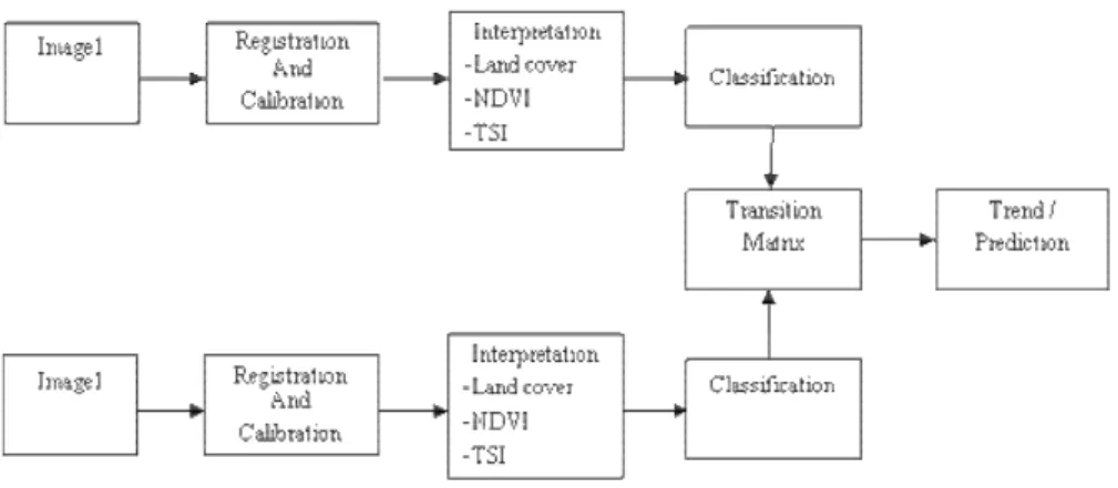
Markov model of change detection of Seasonal Land Cover change in Serang, Banten
Figure 2: Flowchart of Markov change detection technique.
Transitional Matrix and Probability Matrix
Build Markov Model of Change Detection Use 6 by 6 matrix for transitional matrix and probability matrix analyses (6 by 6 indicates a number of land cover classes). To be note, that this classification must apply the same to the other images. Counted the number of pixel in each classes of each image and generated the probability matrix.
RESULTS AND DISCUSSION
Land Cover Classification
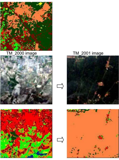
In this task aim is to see the changing in land, not in the ocean. Unfortunately, the oceans in these two images have their own reflectance, so the ocean cannot classify as one object as water body. Like it can see from the picture in Figure 3.
15
This image has been through the unsupervised classification, and the ocean has three different classes (purple, dark blue, and light blue). The analysis of ocean remote sensing will be discussed in next task, it will not discussed now. This image is the image from year 2000. Since it only wanted to detect the change in land, which is contain of 6 classes (forest, plantation, paddy field, bareland, residential, fishpond), while the ocean itself has make 3 classes, so in this image it will made 9 classes so in the land there will be 6 classes of object. The unsupervised classification is used, instead of supervised classification, because it is hard to determine the bareland, residential area, and the paddy field.The image acquired in April, the end of rainy season. In this month farmer usually begin the seedling activity. In this condition, the paddy field will full content of wet soil that has close reflectance to the bareland. Especially when the image is capture after raining, the different between paddy field and the bareland that is also wet, will be more difficult to determine. Especially because this is Landsat image which have low resolution (30m x 30m). The determining of classes is by looking the pattern of the classification. Fishpond, forest, plantation is easier to identify, while bareland, paddy field, and residential is harder to determine.
After seeing the pattern of the class and comparing it to image in 2001, it may be concluded that for residential area, the pattern is usually spread long the road. Residential area also cannot change to another land cover instantly (the interval of two images is only 16 months), so if it is compared to image 2001, there will be a pattern that are similar. It is represent in dark red color (Figure 4).
TM_2000 image TM_2001 image
Figure 4: Defining the residential class.
Dark Pixel Corrected Images
17
Markov model of change detection has been applied to model of change detection of seasonal land cover change from 2000 to 2001 in Serang, Banten. To generate land cover classification, supervised classification was applied, and 20 spectral clusters were generated. The 20 spectral classes created by the algorithm were assigned to informational classes, and aggregated into six classes: forest / plantation, based on the available point data for the region. The information classes defined in this classification were forest, rangeland, crop land, streambed, bare soil, and inundated.As results of such Markov model including Transition Matrix of land cover changes from year 2000 to 2001, Transition Probability Matrix of land cover changes from year 2000 to2001 are shown in
Table 1 and
Table 2, respectively, from which the occurrences of land cover changes from a certain class to different classes in pixels can be interpreted. From this table revealed that the number of forest or plantation area increased during the period, which is approximately 55% of bare land changed to forest or plantation.
Table 1: Land Cover Changes: Transition Matrix of year 2000 to 2001 (in ha)
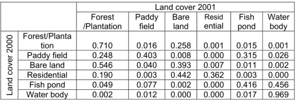
Table 2: Land Cover Changes: Transition Probability Matrix of year 2000 to 2001
Land cover 2001
/Plantation Forest
Paddy field
Bare land
Resid
ential pond Fish
Water body Forest/Planta
tion 0.710 0.016 0.258 0.001 0.015 0.001
Paddy field 0.248 0.403 0.008 0.000 0.315 0.026 Bare land 0.546 0.040 0.393 0.007 0.011 0.002
Residential 0.190 0.003 0.442 0.362 0.003 0.000
Fish pond 0.049 0.077 0.002 0.000 0.416 0.456
La nd co ve r 20 00
Water body 0.002 0.012 0.000 0.000 0.017 0.969 Land cover 2001
Plantation Forest / Paddy field Bare land Resid ential pond Fish Water body
Total
Forest/Plantati
on 6535 146 2373 5 135 10 9204
Paddy field 503 820 17 0 639 53 2032
Bare land 4154 305 2993 54 87 15 7609
Residential 23 0 54 44 0 0 121
Fish pond 95 149 4 0 802 879 1929
Land cover 20
00
Water body 50 306 8 0 426 24518 25308
Forest Change
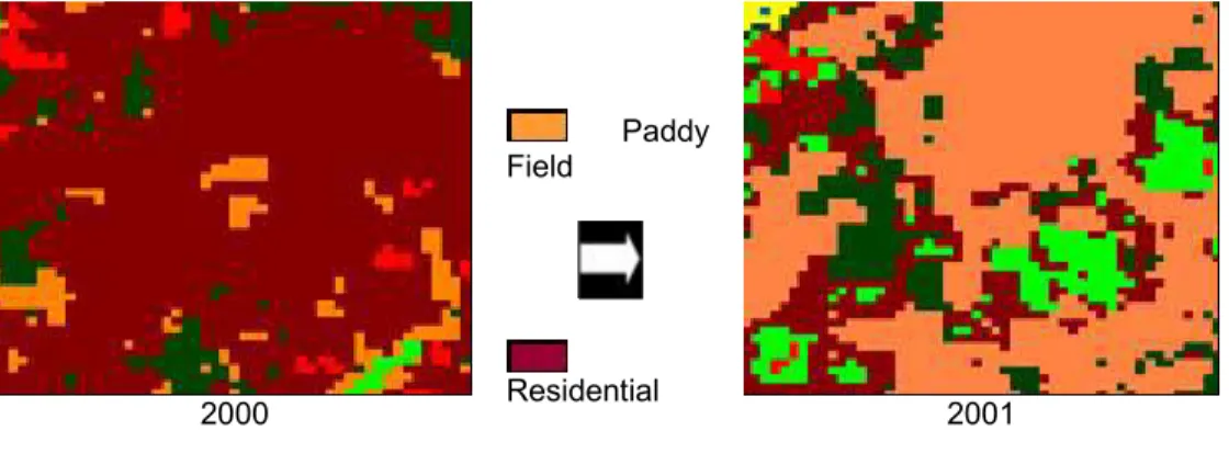
From transition matrix we can see that forest in 2000 is change into two major classes in 2001 (Figure 5): paddy field and residential; 33 % of forest is changing to residential, while 20 % changing to paddy field. This kind of change is logic, because the societies in that area are possibly growing, so they need the new residential area and more paddy field to work on.
2000
Forest
Residential
2001
Figure 5: Forest and residential changes.
Plantation Change
The plantation areas in 2000 have totally changed into other coverages (Figure 6). It was only 1 % that still remains plantation, where about 47% became paddy field, 27% fishpond, and 22 % forest. This change is not a bad change, because the changing is useful for society. Maybe in year 2000 the paddy plant that is still growing becomes one class into plantation. The reflectance of plantation and growing paddy are becoming near value of digital number so it will become one class. It will explain reason why the biggest change is into paddy field. Plantation become forest, after 16 months, the growth of plantation make the density of the plant higher, and will be catch by the sensors of satellite as forest. Plantation become fishpond, maybe because the expansion of society in building the fishpond.
2000
Plantation
Paddy Field
19
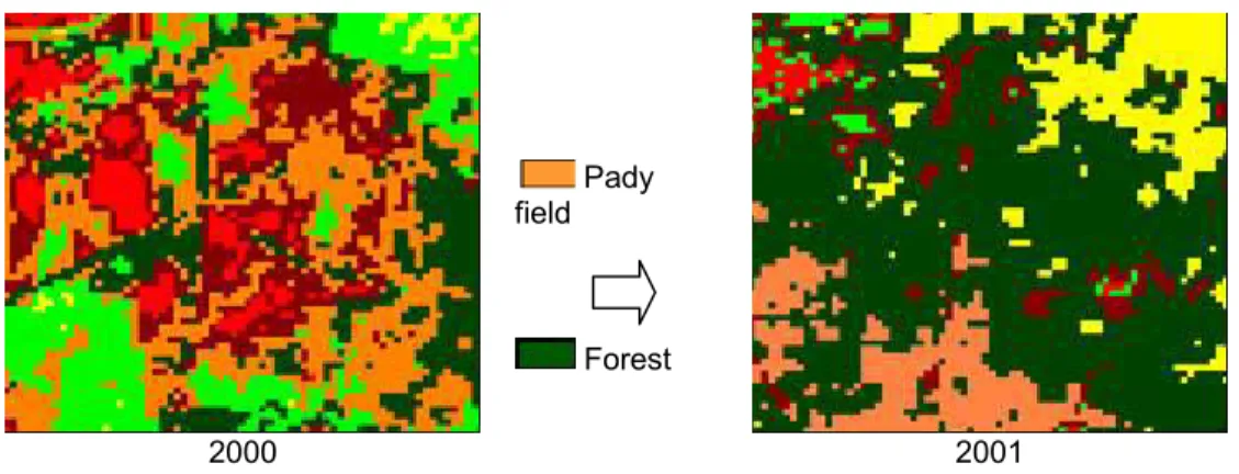
Figure 6: Plantation and Paddy Field changes.Paddy Field
In 2000 like have discuss above, It was very difficult to determine the difference between paddy field, residential, and bare land. This is possibly because when the image was captured, the objects on earth were wet because of the rain. This condition would effect the reflectance of the objects to sensors of satellite. In the transition probability matrix, it said that in this case the paddy field in 2000 changing into forest 24 % and residential 22 %. It might happen when the paddy plant grow in high density so the reflectance was near to the forest’s reflectance. The paddy fields became residential. This could also happen because of the growth of the society. See Figure 7.
2000
Pady field
Forest
2001
Figure 7: Paddy Field Changes.
Bareland
Because in 2000 the paddy field still in early cultivation period, some of the paddy field will look like bareland (Figure 8). It is shown from the matrix that 42 % of bareland changed into paddy field while 23 % changed into plantation.
2000
Bareland
Paddy Field
Figure 8: Bareland Changes.
Residential
The residential changed by 34 % into paddy field, and 24 % into plantation (Figure 9). Like we discuss above, residential in 2000 might be bareland or paddy field. So, if the residential suddenly change 34 % to paddy field in just 16 months (which is almost impossible in Indonesia, usually paddy field that is changed into residential), it might be happens because it was paddy field in 2000 but because of the condition, it was classed as residential. And residential changing 24 % into plantation can possibly happen because it is not residential but bareland that become plantation area, or paddy field that contains of paddy plants in middle density.
Fish pond
Compare to another class, the fishpond is not change much. The much change only happens 7 % into paddy field. Changing fishpond to paddy field is usually happens when the water is no longer enough to fill the pond, so the farmer will change it into paddy field.
2000
Paddy Field
Residential
2001
Figure 9: Residential Changes.
SUMMARY
Few factors might have caused errors in the classification of land cover using satellite images, especially when it is faced with multi temporal images having different spectral characteristic due to scanning in different seasons. Another factor, such as relief can lead to image distortions in mountainous regions, while slope and aspect can influence the natural variability.
21
the change information from satellite data relies on effective and accurate change detection techniques.Markov is a good technique having great capability on generating information relating to changes of specific themes. Markov is one application of change detection that can be used to predict future changes based on the rates of past change.
REFERENCES
Aavikson, K. 1995. Simulating Vegetation Dynamics and Land Use in a Mire Landscape Using a Markov Model. Landscape and Urban Planning, 31: 129 – 142.
Jensen, J.R. 2000. Remote Sensing of the Environment. An Earth Resource Perspective. Prentice-Hall. Upper Saddle River, New Jersey. 542pp.