Seasonal changes in the PM1 chemical composition north of Mexico City

(1)

Seasonal changes in the PM

1

chemical composition north of Mexico City

Franco GUERRERO,1_{Harry ALVAREZ-OSPINA,}2_{Armando RETAMA,}3_{Alfonso LÓPEZ-MEDINA,}3

Telma CASTRO4_{and Dara SALCEDO}1*

1_{UMDI-Juriquilla, Facultad de Ciencias, Universidad Nacional Autónoma de México, Boulevard Juriquilla 3001,} 76230 Juriquilla, Querétaro, México

2_{Facultad de Ciencias, Universidad Nacional Autónoma de México, Circuito Exterior s/n, Ciudad Universitaria, 04510} Ciudad de México, México

3_{Dirección de Monitoreo Atmosférico, Secretaría del Medio Ambiente, Av. Tlaxcoaque 8 piso 6, 06090 Ciudad de} México, México

4_{Centro de Ciencias de la Atmósfera, Universidad Nacional Autónoma de México, Circuito de la Investigación} Científica s/n, Ciudad Universitaria, 04510 Ciudad de México, México

* Corresponding author; email: dara.salcedo@ciencias.unam.mx

Received:December 16, 2016; accepted: May 25, 2017

RESUMEN

Se instaló un Monitor de Especiación Química de Aerosoles (ACSM, por sus siglas en inglés; Aerodyne Inc.) en un sitio al norte de la Ciudad de México del 13 de noviembre de 2013 al 30 de abril de 2014, con el objetivo de investigar la variabilidad estacional de la composición química del aerosol menor a 1 µm. El ACSM determina la concentración en masa, en tiempo real, de las especies más importantes (nitrato, sulfato,

amonio, cloruro y compuestos orgánicos) del material particulado no refractario menor a 1 µm (NR-PM1),

con una resolución temporal de 30 min. Durante dicho periodo también se midieron variables meteorológicas (temperatura, humedad relativa, y dirección y velocidad del viento), y las concentraciones de carbono negro,

PM1, PM2.5, CO, SO2, NO, NO2 y O3. La concentración en masa de NR-PM1 sumada a la concentración

del carbono negro (que debe ser cercana a la concentración total de PM1) tuvo una buena correlación con la

concentración medida con un equipo de microbalanza de elemento oscilatorio, lo cual indica la buena calidad de los datos del ACSM. En promedio, la composición del aerosol, así como su variabilidad diurna fueron similares a lo encontrado en campañas anteriores en las que se usó instrumentación similar (MCMA-2003 y MILAGRO). Sin embargo, el aerosol mostró un carácter ácido durante noviembre y diciembre, probablemente debido a una mayor humedad relativa, menor temperatura, y vientos más frecuentes del noroeste (donde se encuentra el complejo industrial Tula) durante este periodo. Una baja concentración de amoniaco en la fase

gas (NH3) también puede tener un efecto importante en la acidez observada. Estos resultados sugieren un

cambio estacional en la química del aerosol, el cual debe verificarse llevando a cabo más estudios a largo plazo.

ABSTRACT

An Aerodyne Aerosol Chemical Speciation Monitor (ACSM; Aerodyne Inc.) was deployed at a site north of Mexico City from November 13, 2013 to April 30, 2014 to investigate the seasonal variability of the chemical composition of submicron particles. The ACSM provides real time information on mass concentration of the non-refractory main species (nitrate, sulfate, ammonium, chloride and organic compounds) in particulate

mat-ter less than 1 μm (NR-PM1) with a 30-min time resolution. Meteorological variables (temperature, relative

humidity, and wind speed and direction), as well as concentrations of black carbon, PM1, PM2.5, CO, SO2, NO,

NO2, and O3, were also measured. The total NR-PM1 mass concentrations plus black carbon (which must be

close to the PM1 total mass) showed a good correlation with PM1 mass concentration measured with a Tapered

(2)

similar instruments (MCMA-2003 and MILAGRO). However, it was observed that the aerosol was persistently acidic during November and December probably due to a higher relative humidity, lower temperature, and more frequent winds from the NW, where the Tula industrial complex is located. A lower concentration of ammonia

(NH3) in the gas phase might affect the PM acidity too. These results suggest a seasonal variability in the aerosol

chemistry in Mexico City, which should be verified with more long-term studies.

Keywords: ACSM, NR-PM1 chemical composition, aerosol acidity, Mexico City.

1. Introduction

The Mexico City Metropolitan Area (MCMA) is on average 2240 masl at 19º 29’ N and 99º 90’ W, in a basin surrounded by mountains, but relatively open to the north. There are more than 21 million inhabitants,

and every year are emitted close to 27 706 ton of PM10

and 9 847 ton of PM2.5 to the atmosphere (SEDEMA,

2016a). Being one of the largest megacities in the world, the MCMA can have significant impacts on human and ecosystems health, as well as on global change (Baklanov et al., 2016). Because of this, two major campaigns in the city have been organized focusing on understanding the processes and global effects of the city emissions: MCMA-2003 (Molina et al., 2007) and MILAGRO (Molina et al., 2010). MCMA-2003 was carried out in the spring of 2003 and, among other instruments, an Aerodyne Aerosol Mass Spectrometer (AMS) was deployed for the first time in Mexico with the objective of studying the chemical composition of the aerosol with a high time resolution. In such study, Salcedo et al. (2006) found that the organic fraction of the Mexico City aerosol was the largest, followed by the inorganic fraction (nitrate, sulfate, ammonium, and chloride). In general, sulfate and nitrate were neutralized by ammonium, except for some short periods with high sulfate concentration, which showed an acidic nature. The diurnal variability of the aerosol components was also analyzed showing that nitrate concentration was dependent on the photochemical activity, while sulfate concentration had a regional character. The variabil-ity shown by the organic fraction was explained by a combination of primary emissions and secondary production. During MILAGRO, in the spring of 2006, Aiken et al. (2009) again deployed an aerosol mass spectrometer in Mexico City. Their observations were consistent with those from MCMA-2003. In addition, they performed a detailed analysis of the organic fraction of the aerosol, identifying four components: a primary hydrocarbon-like component (HOA); an

oxygenated component, probably of secondary origin (OOA); a component corresponding to biomass burn-ing (BBOA); and a small local nitrogen-containburn-ing fraction (LOA). Both campaigns took place during the spring, for only few weeks, in one specific site each one. Since 2006, there has not been another similar study. Hence, on spite of all the knowledge generated during MCMA-2003 and MILAGRO, there is still a lack of information regarding the seasonal variability of the aerosol chemical properties in Mexico City.

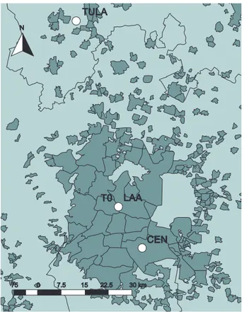
In this paper, we present the results from ground-based measurements at a site north of Mexico City (very close to the MILAGRO supersite, T0) for a period of almost six months, during the winter of

2013-2014. PM1 chemical concentrations and

com-position were measured with an Aerosol Chemical Speciation Monitor (ACSM), the most robust version of the AMS. This data, together with criteria pollut-ants concentrations and meteorological variables, was analyzed in order to look for seasonal changes in the aerosol chemistry. The ACSM data was compared to results from Salcedo et al. (2006) and Aiken et al. (2009) from MCMA-2003 and MILAGRO cam-paigns, respectively.

2. Methodology 2.1 Site

(3)

2.2 Aerosol Chemical Speciation Monitor

The Aerosol Chemical Speciation Monitor (ACSM; Aerodyne Research Inc., Billerica MA) is an aero-sol mass spectrometer (AMS) capable of measuring chemical composition of non-refractory submicron

particulate matter (NR-PM1) (Ng et al., 2011),

which includes all species that can evaporate in

few seconds at ~600 o_{C under vacuum (the}

tem-perature of the vaporizer within the instrument). Specifically, the ACSM detects nitrate, sulfate, ammonium, chloride, and the organic fraction of the aerosol; it does not detect components such as sea salt, soil dust, and elemental carbon (Jiménez et al., 2003). For this study, the ACSM was calibrated following the procedures described by Ng. et al. (2011), using ammonium nitrate and ammonium sulfate. Air was sampled at the roof of the principal building at LAA (4.5 m above ground level) using a Teflon coated aluminum cyclone with a 2.5 µm

cut point at 5 LPM (model 1270; URG corporation, Chapel Hill NC). A multi-tube Nafion dryer (model PD-50T-12-MSS; Perma Pure LLC, Lakewood NJ) was installed right before the ACSM inlet to dry the aerosol. The data acquisition program was set for a time resolution of ~30 min. For the data analysis, a collection efficiency (CE) equal to 0.5 was used because this value was successfully used in previous campaigns in Mexico City using AMS

technology. The uncertainties for the NR-PM1 are

estimated to be –30 to +10% (Salcedo et al., 2006; Aiken et al., 2009).

2.3 Other instruments

Along with the ACSM, other instruments were located on the roof of the LAA building from No-vember 13, 2013 until March 31, 2014. Particulate matter total concentration was measured using two Tapered Element Oscillating Micro-Balances (TEOM, model 1400AB equipped with a Filter Dynamics Measurement System 8500C; Thermo Scientific, Franklin MA), with 2.5 and 1 µm cut point cyclones (VSCC; BGI, Butler NJ) for size

selection. TEOM has a precision of ±2.5 μg m–3

for 1-h averages. Additionally, en aethalometer (AE33 2008; Magee Scientific, Berkeley CA) with

a selective inlet for PM2.5 (SCC1.829; BGI, Butler

NJ) was used to detect black carbon (BC). The BC mass concentration was calculated from the change in optical attenuation at the 880 nm channel using

a mass absorption cross section of 7.77 m2_g–1_{. The}

precision of this measurement was < 10%.

In addition to the particle instruments, the

follow-ing gases were measured: CO, SO2, NO and NO2,

and O3 (Serinus30, Serinus50, Serinus40, Serinus10,

respectively; Ecotech Pty Ltd, Knoxfield Australia). Temperature (T) and relative humidity (RH) were measured using a sensor (083E; Met One Instruments, Grants Pass OR) located inside an aspirated radiation shield positioned 4 m above ground level on a mete-orological tower. For wind speed (WS) and direction (WD) a lightweight three-cup anemometer and vane (010C and 020C; Met One Instruments, Grants Pass OR) were placed on top of the 10-m tower.

Figures S1 and S2, in the supplemental material, show the time series of the above meteorological variables and pollutants concentrations during the campaign.

0 7.5 15 22.5

TULA

N

30 km 75

T0 LAA

CEN

(4)

2.4 General remarks

All concentrations are reported in local temperature and pressure conditions. The time used corresponds to Coordinated Universal Time minus 6 h (UTC-6). Before April 6 this time corresponded to local time. However, Daylight Savings Time started on April6; after that, local time corresponded to UTC minus 5 h (UTC-5). We used the built-in fitting routines included in Igor Pro 6.36 data analysis software (Wavewmetrics, 2014) for the statistical analysis. In all cases, we use Pearson´s r (r) to describe the linear dependence between two variables.

3. Results and discussion 3.1 PM concentrations

The ACSM only detects the non-refractory material

in PM1; hence, assuming that BC was mainly in the

submicrometric fraction (Schwarz et al., 2008), we added the ACSM total (sum of nitrate, sulfate, am-monium, chloride and organics) and the black carbon concentrations (ACSM + BC) in order to obtain a

bet-ter estimate of the PM1 mass concentration. The result

was compared to the PM1 TEOM measurements in

Figure 2. There is a good linear correlation between

ACSM + BC and PM1 (r = 0.91), which is a sign of

the soundness of the data. ACSM + BC concentration

is ~20% lower than the PM1 (the slope of the fitted

line is 0.81), probably because of the refractory ma-terial (dust and metals) not accounted for in ACSM + BC. For example, in previous similar studies in Mexico City (MCMA-2003 and MILAGRO) it was estimated that the mineral material (which included metals and soil) accounted for approximately 7-8 % of the fine aerosol (Salcedo et al., 2006; Aiken et al.,

2009). Experimental uncertainties of each instrument, as well as differences in inlets design and position, might also contribute to the difference observed.

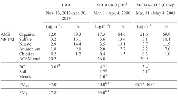
Average concentrations of total NR-PM1, BC, and

PM concentrations measured in this study are shown in Table I. The average concentrations and mass

fractions of the main NR-PM1 components from this

campaign, as well as from the MCMA-2003 (Salcedo et al., 2006) and MILAGRO (Querol et al., 2008; Aiken et al., 2009) campaigns are also included in the table, showing that all comparable values are on the same order of magnitude during the three campaigns. The differences observed might be explained by year-to-year variability and site location. The yearly variability of the PM concentrations in Mexico City is illustrated in Figure S3 in the supplemental

mate-rial, where PM2.5 monthly concentrations measured

in two sites of the Mexico City’s Red Automática de Monitoreo Atmosférico (Air Quality Monitoring Network) from 2003 to 2015 are plotted (SEDE-MA, 2016b). Camarones (CAM; 19º 28’ 06.18’’ N, 99º 10’ 10.95’’ W) and UAM Iztapalapa (UIZ; 19º 21’ 38.90’’ N, 99º 04’ 25.96’’ W) sites were chosen because they are the nearest stations to LAA and CEN sites, respectively. The standard deviations of the concentrations for the same month in the same site were in the range of 10 to 20%, depending on the month; differences between the two sites were as large as 30% for the same monthly period. It is also important to note that PM concentrations shown in Table I for different campaigns were measured using different instruments such as TEOMs, optical particle counters (OPC, Grimm; Ainring, Germany), and Dusttrak Aerosol Monitors (TSI Inc.; Shoreview, 160

120

80

40

0

13/11/13 4/12/13 25/12/13 15/1/14 5/2/14 26/2/14 19/3/14

a b

TEOM PM1 (µg m–3)

ACSM +BC (µg

m

–3)

Day/Month/Year

Mass concentration (µg

m

–3)

0

1:1

Linear fit y = 0.81x r = 0.91

40 80 120

0 40 80 120 ACSM+BC

TEOM PM1

Fig. 2. Time series and scatter plot of ACSM + BC and PM1 mass concentrations at LAA. The vertical dotted

(5)

MN). The variety of instruments used might also affect the comparisons among campaigns due to the inherent uncertainties of each of them. Finally, con-centrations of the non-refractory material measured in the previous campaigns are also shown in Table I as a reference for the material that was not accounted for by the ACSM. Unfortunately, we do not have information on this fraction of the aerosol for the 2013-2014 campaign.

Data in Table I show that the average

composi-tion of NR-PM1 during the campaign was similar to

previous campaigns: i.e., the organic component is the largest one, followed by sulfate, nitrate, and am-monium. Chloride comprises only 1% of the mass. Figure 3 shows the time series of the concentrations

of the main NR-PM1 components and their mass

fraction. In general, nitrate and ammonium showed a diurnal trend that was not as clear for the rest of the components. Nitrate concentration was higher in November and December compared to the rest of the campaign. Sulfate displayed periods of elevated concentrations that lasted few hours to several days; these periods were more common during the first half of the campaign. In general, chloride was pres-ent in very low concpres-entrations; however, two large spikes were observed on December 25 and January

1, which were accompanied by high concentrations of sulfate, probably due to the Christmas and New Year’s fireworks (Drewnick et al., 2006).

3.2 PM1 acidity

In order to determine the acidity of the NR-PM1,

we calculated the predicted ammonium needed to completely neutralize the sulfate, nitrate and chloride present in the aerosol, using the following equation:

NH4_pred = 18

(

+

)

2[SO42–]

96

[NO3–]

62 +

[Cl–_]

35.5 (1)

where [SO42–], [NO3–], and [Cl–] are the

concentra-tions of sulfate, nitrate, and chloride in µg m–3_{. This}

equation assumes that the inorganic anions are in

the form of neutralized ammonium salts: NH4NO3,

(NH4)2SO4, NH4Cl. We also calculated the missing

ammonium for neutrality using the following equa-tion:

NH4_miss = NH4_pred - NH4_meas (2)

where NH4_meas is the measured ammonium

con-centration in µg m–3_{. The time series of NH}

4_miss

Table I. Average PM mass concentrations and percent composition from this study (LAA), and from MILAGRO and MCMA-2003 campaigns.

LAA MILAGRO (T0)1 _{MCMA-2003 (CEN)}2

Nov. 13, 2013-Apr. 30,

2014 Mar. 1 - Apr. 4, 2006 Mar. 31 - May 4, 2003

(µg m−3₎ _% _{(µg m}−3₎ _% _{(µg m}−3₎ _%

AMS

NR-PM1

Organics 12.0 59.3 17.3 64.6 21.6 69.9

Sulfate 3.2 16.1 3.6 13.4 3.1 10.1

Nitrate 2.9 14.4 3.5 13.1 3.7 11.9

Ammonium 1.8 9.0 2.0 7.7 2.2 7.0

Chloride 0.2 1.2 0.4 1.5 0.3 1.0

ACSM total 20.2 26.8 30.9

BC 3.03Ŧ _4.2* _3.4*

Soil 1.7§ _2.1Ŧ

Metals 1.0Ŧ

PM2.5 37.0a 40.0b,3 35.7a, 40.0c

PM1 27.8a 33.0b,3

Ŧ _PM

2.5; * PM2.0; § PM1; a TEOM; bOPC; c Dusttrak; 1 Aiken et al., 2009; 2 Salcedo et al., 2006; 3 Querol

(6)

is presented in Figure 4a, where it is evident that

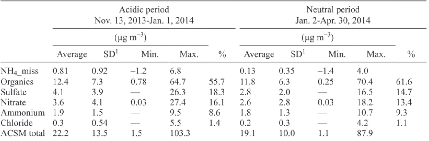
NH4_miss was persistently higher at the beginning

of the campaign than at the end (see also Table II and

Fig. 5). In fact, when plotting NH4 vs NH4_pred, the

data points before January 2, 2014 (Fig. 4b) lie below the 1:1 line, indicating that there is not enough am-monium to neutralize the sulfate, nitrate and chloride; i.e. the aerosol is acidic. In fact, we recalculated the predicted ammonium assuming that sulfate is in the

form of ammonium bisulfate (NH4HSO4):

NH4_pred_bs = 18

(

+

)

[SO42–]

96

[NO3–]

62 +

[Cl–_]

35.5 (3)

When NH4_pred_bs is plotted vs. NH4_meas

(Fig. 4c), the fitted line has a slope closer to 1. After January 2, 2014 (Fig. 4d), the aerosol can be con-sidered neutral.

The results for the second period of the campaign are consistent with observations during MCMA-03 and MILAGRO campaigns, when the aerosol was also found to be neutral in March and April 2003

and 2006 (except for one week in 2003) (Salcedo et al., 2006; Aiken et al., 2009). However, this is the first report of a persistent acidity in the Mexico City aerosol. It would be important to repeat this kind of long-term campaigns for several years in order to determine if this is a yearly trend.

Table II includes the average concentrations of ACSM components during the acidic and neutral pe-riods, as described in the previous paragraph. During the acidic period, sulfate and nitrate concentrations were larger than during the neutral period, while am-monium concentrations were similar, which explains the difference in acidity observed.

In order to look for the conditions that might be responsible for the observed change in acidity, the Kruskal-Wallis (KW) test was used (with a confidence level of 99%) to determine if there were statistically significant differences in the parameters measured during the two periods. We also draw box-and-whisker plots of the same parameters for an easier visualization of the differences. Figure 5 shows the plots for the parameters that might be more related with aerosol acidity, and Figure S4 for the 120

0

13/11/13 4/12/13 25/12/13 15/1/14 5/2/14 26/2/14 19/3/14 9/4/14 30/4/14

Day/Month/Year 10

5

0 20

0

1

0

Mass fraction

6

0 20

0

chloride

ammonium

sulfate

nitrate

ACSM total / organics

m

–3)

Fig. 3. Time series of the main NR-PM1 components and their mass fraction at LAA. The vertical dotted

(7)

rest. The KW test indicated that all parameters were statistically different between periods, except for ammonium, organics, and wind speed. These results confirm the discussion regarding concentrations of

NH4_miss, nitrate, sulfate and ammonium discussed

above. SO2 and NOx concentrations, precursors of

sulfate and nitrate respectively, were higher during the acidic period. In addition, the RH was higher, and the T lower; both of which conditions can be related

to higher concentrations of sulfate and nitrate due

to faster oxidation rates, and the HNO3 gas-particle

equilibrium shifting to the condensed phase (Seinfeld and Pandis, 2012). Finally, the wind roses shown in Figure 6 reveal more frequent, and faster winds from the NW affecting the LAA during the acidic period. These winds might also affect the amount of sulfate observed because they come from the direction of the Tula industrial complex (see Fig. 1), which is one of 8

6 4 2

0 –2

13/11/13 4/12/13 25/12/13 15/1/14 5/2/14 26/2/14 19/3/14 9/4/14 30/4/14 Day/Month/Year

acidic period neutral period

a NH4_miss

12 8 4 0

NH4_pred_bs (µg m–3₎ 1:1 c

Linear fit y=0.94x r=0.97

12 8 4 0

NH4_pred (µg m–3₎ 1:1

Linear fit y=0.94x r=0.96 d

12

8

4

0

12 8 4 0

NH4_pred (µg m–3₎ 1:1

Linear fit y=0.68x r=0.95 b

m

–3)

NH4_meas (µg

m

–3)

Fig. 4. (a) Time series of NH4_miss (Eq. 2). (b) and (c) NH4_meas vs. NH4_pred, and vs. NH4_pred_bs (Eqs. 1 and 3) during the acidic period. (d) NH4_meas vs. NH4_pred (Eq. 1) during the neutral period. The solid lines in panels b-d correspond to the fitted lines, and the dotted lines to 1:1 lines.

Table II. Summary of the composition of NR-PM1 for the acidic and neutral periods at LAA. Minimum values without

a value indicate signals within the noise level. Acidic period

Nov. 13, 2013-Jan. 1, 2014 Jan. 2-Apr. 30, 2014Neutral period

(µg m−3₎ _{(µg m}−3₎

Average SD1 _Min. _Max. _% _Average _SD1 _Min. _Max. _%

NH4_miss 0.81 0.92 –1.2 6.8 0.13 0.35 –1.4 4.0

Organics 12.4 7.3 0.78 64.7 55.7 11.8 6.3 0.25 70.4 61.6

Sulfate 4.1 3.9 — 26.3 18.3 2.8 2.0 — 16.5 14.7

Nitrate 3.6 4.1 0.03 27.4 16.1 2.6 2.8 0.03 18.2 13.4

Ammonium 1.9 1.5 — 9.5 8.6 1.8 1.3 — 10.7 9.3

Chloride 0.3 0.54 — 5.5 1.4 0.2 0.3 — 4.2 1.1

ACSM total 22.2 13.5 1.5 103.3 19.1 10.0 1.1 87.9

(8)

the most important SO2 sources in Mexico City (de Foy et al., 2009). In conclusion, the higher acidity observed at the beginning of the campaign might be

related to higher SO2 and NOx concentrations, higher

RH, lower T, and more frequent winds from the NW. In fact, high relative humidity and northerly winds were also observed during the week in 2003 when acidic aerosols were detected during MCMA-2003 (Salcedo et al., 2006).

In Figure 7 we plotted NH4_miss vs. sulfate and

nitrate. While NH4_miss shows a good correlation

with sulfate (r = 0.9093), it does not correlate at all with nitrate, which can be explained by the complex

5 4 3 2 1 0 ammonium 12 8 4 0 nitrate 12 10 8 6 4 2 0 sulfate 250 200 150 100 50 0 ppb ºC NOx 40 30 20 10 0 ppb SO2 3.0 2.0 1.0 0.0 NH4_miss 25 20 15 10 T 80 60 40 20 % RH

m

–3)

m

–3)

m

–3)

m

–3)

Fig. 5. Box-and-whisker plots for several parameters measured during the acidic (grey) and neutral (black) periods. Whiskers correspond to 5 and 95 percentiles; vertical lines to 25, 50, and 75 percentiles; and circles to the average value. KW tests indicated that all parameters shown here were sta-tistically different between periods, except for ammonium.

1 N S W E 0. N S W E 0.05 0. 0.15 0.05 1 0.15

wind speed (m/s) 0-1 1-2 2-3 3+

acidic period neutral period

Fig. 6. Wind roses during the acidic and neutral periods. The radial axes in the wind rose indicate frequency of winds.

30 20 10 0

nitrate (µg m–3₎ 8 6 4 2 0 30 20 10 0

sulfate (µg m–3₎ linear fit r = 0.9093

NH

4

_miss (µg

m

–3)

(9)

phase and acid-base equilibriums of the system

(H2SO4 + HNO3 + NH3 + H2O) (Seinfeld and Pandis,

2012). Sulfuric acid is non-volatile and exists mainly in the condensed phase (solid or liquid); on the other hand, nitric acid and ammonia partition between the gas and the condensed phases, depending on the RH, temperature, and the total concentration of all the species in the system. In general, under ammonia-rich

conditions, NH3 will neutralize H2SO4 and HNO3

to form sulfate, nitrate, and ammonium, which can be aqueous or forming salts depending on the RH.

However, in the case of insufficient NH3 the sulfuric

acid will tend to be partially neutralized (as bisulfate) and the nitric acid will be forced to the gaseous phase. During the MILAGRO campaign, Fountoukis et al. (2009) found that the atmosphere in the MCMA was unusually ammonia-rich, which was used to explain the neutrality of the aerosol back then. In contrast, Figure 7 suggests that, during November and De-cember 2013, the ammonia present in the atmosphere was not enough to neutralize the nitric and sulfuric acids. This suggestion is consistent with results from

Cady-Pereira et al. (2017), who calculated NH3

concentrations over Mexico City during 2013-2015 using the Tropospheric Emission Spectrometer (TES)

instrument on the NASA AURA satellite, and found

a seasonal trend in NH3 concentrations, with a

min-imum during September-November and a maxmin-imum in March-May. Cady-Pereira et al. (2017) results not only shed light on the reason for the aerosol acidity observed during 2013, but indicate a probable yearly trend. Again, it would be important to perform more campaigns to verify this hypothesis.

The acidity of the aerosol has wide implications that span from effects to human and ecosystems health, to measures to control particle concentra-tions through emissions regulation. Also, the pH of aerosols can change the chemistry occurring in the atmosphere through heterogenous acid-catalyzed re-actions, and increase solubility of material associated with mineral dust (Weber et al., 2016). Hence, it is important to better understand the variability of the PM acidity, as well as the factors that determine it, which can only be done with more long-term studies such as this one.

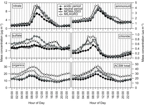
3.3 NR-PM1 diurnal cycles

Average diurnal plots of the main NR-PM1

compo-nents in 2013-2014, 2006 (Aiken et al., 2009), and 2003 (Salcedo et al., 2006) are shown in Figure 8.

6

4

2

0

sulfate 1.0

0.8 0.6 0.4 0.2 0.0 chloride

30

20

10

0

00:00 02:00 04:00 06:00 08:00 10:00 12:00 14:00 16:00 18:00 20:00 22:00

Hour of Day organics

12

8

4

0

nitrate 5₄

3 2 1 0 ammonium

50 40 30 20 10 0

00:00 02:00 04:00 06:00 08:00 10:00 12:00 14:00 16:00 18:00 20:00 22:00

Hour of Day

ACSM total acidic period

neutral period MCMA-2003 MILAGRO

m

–3)

m

–3)

Fig. 8. Average diurnal cycles of the NR-PM1 components at LAA (acidic and neutral

(10)

The plots show the hourly average concentrations of all the data available for each period. Figures S5 and S6 show the diurnal box-and-whisker plots for the diurnal concentrations during the acidic and neutral periods, respectively. In general, as for the average concentrations discussed in section 3.1, the behavior of all the components were similar during the three campaigns. Nitrate shows a maximum concentration in the morning, which corresponds to the photochem-ical activity, and it is closely followed by ammoni-um. The organic fraction also shows a maximum at midday, but the raise starts earlier in the morning due to the primary emissions by vehicles; i.e., its diurnal cycle is a combination of primary aerosols emitted during the early rush hour, and secondary aerosols formed during the morning. Chloride maximum concentrations occur in the early morning due to its relatively high volatility. Finally, the diurnal cycle of sulfate is determined by its regional nature. The diurnal cycles during acidic and neutral periods are qualitatively similar; however, the absolute values are different, especially for nitrate and sulfate, as discussed in section 3.2.

The sulfate diurnal cycle is compared to the

NH4_miss cycle in Figure 9, where it is evident

that there is a close relation between the acidity of the aerosol and the sulfate concentration during the

acidic period. Such relation is not observed during the neutral period, which is consistent with the dis-cussion in section 5.2.

4. Conclusions

Mass concentration and composition of the NR-PM1

was measured with a 30-min time resolution in a site north of Mexico City for a period of almost six

months. Average PM1 concentrations and

composi-tion in 2013-2014 were in the same order of magni-tude as observed in previous campaigns during the spring of 2003 and 2006. The differences observed might be explained by yearly variability and the dif-ferent location of sites. However, in November and December 2013 the aerosol showed a persistent acidic behavior due to a larger concentration of sulfate and nitrate with respect to ammonium. This observation is consistent with higher RH and lower T during these two months, which promote faster oxidation rates

and the HNO3 gas-particle equilibrium shifting to the

condensed phase. More frequent winds from the NW, where Tula industrial complex is located, might also affect the acidity of the aerosol, because Tula

rep-resents one of the main SO2 sources in Mexico City.

Finally, a seasonal reduction in the concentration of gas phase ammonia during November and December probably inhibited the neutralization processes of the aerosol.

This study represents the longest continuous campaign measuring aerosol composition in Mexico City with a high time resolution. The results suggest a seasonal variability in aerosol acidity that had not been reported before, which could have important implications on human and ecosystems health, as well as on the chemistry occurring in the atmosphere. It would be necessary to perform more long-term campaigns in order to determine if this is a yearly trend. Furthermore, this study exposes the little knowledge that exists regarding chemical processes occurring under different atmospheric conditions in Mexico City, and indicates the importance of long-term studies.

Acknowledgments

This research was supported by program UN-AM-DGAPA-PAPIIT IA100514. F. Guerrero thanks Consejo Nacional de Ciencia y Tecnología (CONA-CyT, México) for his doctoral scholarship.

Fig. 9. Average diurnal cycles of the NH4_miss and sulfate concentrations for the acidic and neutral periods.

2.0

1.5

1.0

0.5

0.0

–0.5 2.0

1.5

1.0

0.5

0.0

–0.5

6

4

2

0 acidic period

00:00 02:00 04:00 06:00 08:00 10:00 12:00 14:00 16:00 18:00 20:00 22:00

Hour of day

6

4

2

0 neutral period sulfate

NH4_miss

NH4_miss (µg

m

–3)

NH4_miss (µg

m

–3)

sulfate (µg

m

–3)s

ulfate (µg

m

(11)

References

Aiken A.C., D. Salcedo, M.J. Cubison, J.A. Huffman, P.F. DeCarlo, I.M. Ulbrich, K.S. Docherty, D. Sueper, J.R. Kimmel, D.R. Worsnop, A. Trimborn, M. Northway, E.A. Stone, J.J. Schauer, R.M. Volkamer, E. Fortner, B. de Foy, J. Wang, A. Laskin, V. Shutthanandan, J. Zheng, R. Zhang, J. Gaffney, N.A. Marley, G. Pare-des-Miranda, W.P. Arnott, L.T. Molina, G. Sosa and J.L. Jiménez, 2009. Mexico City aerosol analysis during MILAGRO using high resolution aerosol mass spectrometry at the urban supersite (T0) – Part 1: Fine particle composition and organic source apportion-ment. Atmos. Chem. Phys. 9, 6633-6653.

doi: 10.5194/acp-9-6633-2009

Baklanov A., L.T. Molina and M. Gauss, 2016. Megacities, air quality and climate. Atm. Environ. 126, 235-249. doi: 10.1016/j.atmosenv.2015.11.059

Cady-Pereira K.E., V.H. Payne, J.L. Neu, K.W. Bowman, K. Miyazaki, E.A. Marais, S. Kulawik, Z.A. Tzom-pa-Sosa and J.D. Hegarty, 2017. Seasonal and Spatial Changes in Trace Gases over Megacities from AURA TES Observations. Atmos. Chem. Phys. Discuss. 2017, 1-31. doi: 10.5194/acp-2017-110.

De Foy B., N.A. Krotkov, N. Bei, S.C. Herndon, L.G. Huey, A.P. Martínez, L.G. Ruiz-Suárez, E.C. Wood, M. Zavala and L.T. Molina, 2009. Hit from both sides: tracking industrial and volcanic plumes in Mexico City with surface measurements and OMI SO2 retrievals during the MILAGRO field campaign. Atmos. Chem. Phys. 9, 9599-9617.

doi: 10.5194/acp-9-9599-2009.

Drewnick F., S.S. Hings, J. Curtius, G. Eerdekens and J. Williams, 2006. Measurement of fine particulate and gas-phase species during the New Year’s fireworks 2005 in Mainz, Germany. Atm. Environ. 40, 4316-4327. doi: 10.1016/j.atmosenv.2006.03.040.

Fountoukis C., A. Nenes, A. Sullivan, R. Weber, T. Van Reken, M. Fischer, E. Matías, M. Moya, D. Farmer and R.C. Cohen, 2009. Thermodynamic characterization of Mexico City aerosol during MILAGRO 2006. Atmos. Chem. Phys. 9, 2141-2156.

doi: 10.5194/acp-9-2141-2009.

INEGI, 2014. Cartografía Geoestadística Urbana. Cierre de los Censos Económicos 2014, DENUE 01/2015, Instituto Nacional de Estadística y Geografía.

Jiménez J.L., J.T. Jayne, Q. Shi, C.E. Kolb, D.R. Worsnop, I. Yourshaw, J.H. Seinfeld, R.C. Flagan, X. Zhang, K.A. Smith, J.W. Morris and P. Davidovits, 2003.

Ambient aerosol sampling using the Aerodyne Aerosol Mass Spectrometer. J. Geophys. Res.: Atmos. 108 doi: 10.1029/2001JD001213

Molina L.T., C.E. Kolb, B. de Foy, B.K. Lamb, W.H. Brune, J.L. Jiménez, R. Ramos-Villegas, J. Sarmien-to, V.H. Paramo-Figueroa, B. Cardenas, V. Gutier-rez-Avedoy and M.J. Molina, 2007. Air quality in North America’s most populous city – overview of the MCMA-2003 campaign. Atmos. Chem. Phys. 7, 2447-2473. doi: 10.5194/acp-7-2447-2007

Molina L.T., S. Madronich, J.S. Gaffney, E. Apel, B. de Foy, J. Fast, R. Ferrare, S. Herndon, J.L. Jiménez, B. Lamb, A.R. Osornio-Vargas, P. Russell, J.J. Schauer, P.S. Stevens, R. Volkamer and M. Zavala, 2010. An overview of the MILAGRO 2006 Campaign: Mexico City emissions and their transport and transformation. Atmos. Chem. Phys. 10, 8697-8760.

doi: 10.5194/acp-10-8697-2010

Ng N.L., S.C. Herndon, A. Trimborn, M.R. Canagaratna, P.L. Croteau, T.B. Onasch, D. Sueper, D.R. Worsnop, Q. Zhang, Y.L. Sun and J.T. Jayne, 2011. An Aerosol Chemical Speciation Monitor (ACSM) for Routine Monitoring of the Composition and Mass Concen-trations of Ambient Aerosol. Aerosol Sci. Tech. 45, 780-794. doi: 10.1080/02786826.2011.560211 Querol X., J. Pey, M.C. Minguillón, N. Pérez, A. Alastuey,

M. Viana, T. Moreno, R.M. Bernabé, S. Blanco, B. Cárdenas, E. Vega, G. Sosa, S. Escalona, H. Ruiz and B. Artíñano, 2008. PM speciation and sources in Mex-ico during the MILAGRO-2006 Campaign. Atmos. Chem. Phys. 8, 111-128. doi: 10.5194/acp-8-111-2008 Salcedo D., T.B. Onasch, K. Dzepina, M.R. Canagaratna, Q. Zhang, J.A. Huffman, P.F. DeCarlo, J.T. Jayne, P. Mortimer, D.R. Worsnop, C.E. Kolb, K.S. Johnson, B. Zuberi, L.C. Marr, R. Volkamer, L.T. Molina, M.J. Molina, B. Cardenas, R.M. Bernabé, C. Márquez, J.S. Gaffney, N.A. Marley, A. Laskin, V. Shutthanandan, Y. Xie, W. Brune, R. Lesher, T. Shirley and J.L. Jiménez, 2006. Characterization of ambient aerosols in Mexico City during the MCMA-2003 campaign with Aerosol Mass Spectrometry: results from the CENICA Super-site. Atmos. Chem. Phys. 6, 925-946.

doi: 10.5194/acp-6-925-2006

(12)

optical size of individual black carbon particles in urban and biomass burning emissions. Geophys. Res. Lett. 35. doi: 10.1029/2008GL033968

SEDEMA, 2016a. Inventario de Emisiones de la CDMX 2014. Contaminantes criterio, tóxicos y de efecto inver-nadero. Secretaría del Medio Ambiente del Gobierno de la Ciudad de México. Available at: http://www.aire. cdmx.gob.mx/descargas/publicaciones/flippingbook/ inventario-emisiones-cdmx2014-2/.

SEDEMA, 2016b. Sistema de Monitoreo Atmosférico. Secretaría del Medio Ambiente del Gobierno de la Ciudad de México. Available at: http://www.aire. cdmx.gob.mx/.

Seinfeld J.H. and S.N. Pandis, 2012. Atmospheric chemis-try and physics: From air pollution to climate change. John Wiley & Sons, 1152 pp.

doi: 10.1021/ja985605y

Wavemetrics, 2014. IGOR Pro V6.36 User’s Guide. Wavemetrics Inc.

(13)

Supplemental material

100

50

20 10 0 4

2

0 13/11/13

WS (ms

–1)T

(ºC)

%RH

4/12/13 25/12/13 15/1/14 Day/Month/Year

5/2/14 26/2/14 19/3/14 0

Fig. S1. Time series of the relative humidity (% RH), temperature (T), and wind speed (WS) at LAA. The vertical dotted arrow separates the acidic and neutral periods (see section 3.2).

4

0 400 200 0 150

0 150

150 0

0 20

0

13/11/13 4/12/13 25/12/13

Day/Month/Year

15/1/14 5/2/14 26/2/14

CO

NO,NO2

SO2

O3

PM2.5

BC

PM1

19/3/14

µg

m

–3

ppb

ppm

(14)

50 40 30 20 10 0

1/04

PM

2.

5

(µg

m

–3)

1/05 1/06 1/07 1/08 Month/Year

1/09 1/10 1/11 1/12 1/13 1/14 UIZ CAM

Fig. S3. Time series of the average PM2.5 monthly concentration, at

two sites of Mexico City’s Red Automática de Monitoreo Atmosféri-co (Air Quality Monitoring Network) (SEDEMA, 2016). UIZ is the closest site in the network to CEN; CAM is the closest to T0 and LAA.

25 20 15 10

10 100

1.2 ₅₀

60

40

20

0 40

30 20 10 0

2.5 2.0 1.5

0.5 0.0 1.0

2.5 2.0

m

s

–1

m

–3)

m

–3)

m

–3)

m

–3)

m

–3)

ppm

ppb 1.5

0.5 0.0 1.0 1.0

0.8 0.6 0.4 0.2 0.0

80 60 40 20 0 8

6 4 2 0 5 0

organics

BC O3 CO WS

chloride total PM1

(15)

nitrate _{ACIDIC PERIOD} ammonium

20 8

6

4 2

0

15

10

5

0

m

–3)

m

–3)

sulfate chloride

Hour of day 20

2

1

0

15 10

5 0

organics ACSM total

20

0:00 2:00 4:00 6:00 8:00 _10:0

0

12:0

0

14:0

0

16:0

0

18:0

0

20:0

0

22:0

0

Hour of day

0:00 2:00 4:00 6:00 8:00 _10:0

0

12:0

0

14:0

0

16:0

0

18:0

0

20:0

0

22:0

0

60

40

20

0

40

0

Fig. S5. Diurnal box-and-whisker plots of the NR-PM1 main species mass concentration, during

(16)

Fig. S6. Diurnal box-and-whisker plots of the NR-PM1 main species mass concentration, during

the neutral period. Whiskers correspond to 5 and 95 percentiles; vertical lines to 25, 50, and 75 percentiles; and circles to the average value.

nitrate _{NEUTRAL PERIOD} ammonium ₆

4

2

0

15

10

5

0

m

–3)

m

–3)

sulfate chloride

Hour of day

1.5

1.0

0.5

0.0

10

5

0

organics _{ACSM total}

20

0:00 2:00 4:00 6:00 8:00 _10:00 _12:00 _14:00 _16:00 _18:00 _20:00 _22:00

Hour of day

0:00 2:00 4:00 6:00 8:00 _10:00 _12:00 _14:00 _16:00 _18:00 _20:00 _22:00

50 40

20

0

40

0

30