(will be inserted by the editor)
Eigenvalues and constraints in mixture modeling:
geometric and computational issues
Luis-Angel Garc´ıa-Escudero · Alfonso Gordaliza · Francesca Greselin ·
Salvatore Ingrassia · Agust´ın Mayo-Iscar
Received: date / Accepted: date
Abstract This paper presents a review about the usage of eigenvalues restric-tions for constrained parameter estimation in mixtures of elliptical distribu-tions according to the likelihood approach. These restricdistribu-tions serve a twofold purpose: to avoid convergence to degenerate solutions and to reduce the onset of non interesting (spurious) maximizers, related to complex likelihood sur-faces. The paper shows how the constraints may play a key role in the theory of Euclidean data clustering. The aim here is to provide a reasoned review of the constraints and their applications, along the contributions of many au-thors, spanning the literature of the last thirty years.
Keywords Mixture Model · EM algorithm · Eigenvalues · Model-based clustering
1 Introduction
Finite mixture distributions play a central role in statistical modelling, as they combine much of the flexibility of non parametric models with nice analytical properties of parametric models, see e.g. Titterington et al. (1985), Lindsay (1995), McLachlan and Peel (2000). In the last decades such models have
Luis-Angel Garc´ıa-Escudero, Alfonso Gordaliza, Agust´ın Mayo-Iscar Department of Statistics and Operations Research andIMUVA University of Valladolid, Valladolid, Spain
E-mail: [lagarcia, alfonsog, agustinm]@eio.uva.es
Francesca Greselin
Department of Statistics and Quantitative Methods Milano-Bicocca University, Milan, Italy
E-mail: francesca.greselin@unimib.it
Salvatore Ingrassia
Department of Economics and Business, University of Catania Corso Italia 55, 95128 Catania, Italy
attracted the interest of many researchers and found a number of new and interesting fields of application. For parameter estimation in mixture models several approaches may be considered, as the ones exposed in McLachlan and Krishnan (2008a). The maximum likelihood (ML) framework is among the most commonly used approaches to mixture parameter estimation, and it is the approach we consider here. In the case of Gaussian mixtures, it is well-known that the likelihood function increases without bound if one of the mixture means coincides with a sample observation and if the corresponding variance tends to zero or, in the multivariate situation, if the variance matrix tends to a singular matrix.
This paper presents a review about the usage of eigenvalues restrictions for constrained estimation, that serves a twofold purpose: to avoid convergence to degenerate solutions and to reduce the onset of non interesting (spurious) maximizers, related to complex likelihood surfaces. From the seminal paper of Hathaway (1985), we will see how the constraints may play a key role in the theory of Euclidean data clustering. The aim here is to provide a reasoned review of the constraints and their applications, along the contributions of many authors, spanning the literature of the last thirty years. Applications of the constraints in robustness, jointly with trimming techniques, requires an extensive discussion per se, hence it will be the argument of a further paper, see Garc´ıa-Escuderoet al.(2017). The plan of the paper is the following. Max-imum likelihood estimation for mixture models is briefly recalled in Section 2, along with conditions assuring the existence and consistency of the esti-mator, in Section 3 different constrained formulations of maximum-likelihood estimation are presented, in Section 4 degeneracy of the maximum likelihood estimation is investigated. The last part of the paper is devoted to the role of eigenvalues in parsimonious models: Gaussian parsimonious clustering models are summarized in Section 5 while in Section 6 mixture of factor analyzers are presented. Finally, conclusions are given in Section 7.
2 Maximum likelihood estimation of parameters in mixture models LetXbe a random vector defined on a heterogeneous populationΩwith values in a d-dimensional Euclidean space. Here, we consider mixtures of elliptical distributions, having density function
p(x;ψ) =π1f(x;θ1) +· · ·+πGf(x;θG) x∈Rd (1)
whereπ1, . . . , πG are themixing weightsand
f(x;θg) =ηg|Σg|−1/2h{(x−µg)Σ−g1(x−µg)} (2)
denotes the density of the elliptical distribution (for more details see, e.g., Fang and Anderson, 1990) whereµg∈Rd andΣg are positive definite matrices in Rd×Rd
the dimensiondof the Euclidean space. Moreover,θg={νg,µg,Σg}belongs
to the same parameter spaceΘ, i.e.θ1, . . . ,θG ∈Θ. Finally, we denote byK
the number of parameters ofψ.
The most popular case of (1) is given byGaussian mixtures, i.e., mixtures with multivariate Gaussian components:
p(x;ψ) =π1φ(x;µ1,Σ1) +· · ·+πGφ(x;µG,ΣG), (3)
where φ(x;µg,Σg) is the density function of the multivariate normal
distri-bution with parameters (µg,Σg). Finally, we set ψ = {(πg,µg,Σg), g =
1, . . . , G} ∈Ψ, whereΨis the parameter space:
Ψ={(π1, . . . , πG,µ1, . . . ,µG,Σ1, . . . ,ΣG)∈RG[1+d+(d
2+d)/2]
: π1+· · ·+πG = 1, πg>0,|Σg|>0 forg= 1, . . . , G}.
(4)
Thus,K= (G−1) +G[1 +d+ (d2+d)/2].
A more general family is given by mixtures of multivariatet distributions, with densities in (2) taking the form
f(x;θg) =
Γ(νg2+d)|Σg|−1/2
(πνg)d/2Γ( νg
2){1 +d(x;µg,Σg)/νg}(νg+d)/2
, (5)
with location parameterµg, a positive definite inner product matrixΣg,
de-grees of freedomνg, and where
d(x;µg,Σg) = (x−µg)Σ−g1(x−µg) (6)
denotes the Mahalanobis distance betweenxandµg, with respect to the
ma-trix Σg. t distributions are progressively becoming popular in multivariate
statistics, providing more realistic tails for real-world data with respect to the alternative Gaussian models. They are a robust alternative able to cope with moderate outliers, as the Mahalanobis distance in the denominator of (5) downweight the contribution of data mildly deviating from the assumed model. For the sake of simplicity, throughout this paper we will generally consider Gaussian mixtures defined in (3). The extension to mixtures oft dis-tributions, and to more general mixtures with elliptical components is usually straightforward.
For a given sample X = {x1, . . . ,xN} of size N drawn from (1), let us
consider the log-likelihood function ofψ,
L(ψ) =
N
n=1
log
G
g=1
πgφ(xn;µg,Σg)
(7)
and denote by
ˆ
ψ= argψ∈ΨmaxL(ψ) (8)
the maximum likelihood estimator (MLE) ofψ.
heterogeneous population and letEP() denote the expectation with respect to P. The aim is to maximize
L∗(ψ) =EP
log
G
g=1
πgφ(·;µg,Σg
(9)
in terms of parameters ψ ∈ Ψ, given in (4). If PN stands for the empirical
measure, PN = (1/N)
N
n=1δ{xn}, where δ{xn} denotes the Dirac function
with probability 1 inxn and 0 elsewhere, we recover the original problem (7)
by replacingP byPN.
The maximum likelihood estimate is usually attained through the EM al-gorithm, that is an iterative procedure for maximizing a likelihood function, in the context of partial information, see e.g. Dempsteret al.(1977); McLach-lan and Krishnan (2008b) for details. The algorithm generates a sequence of estimates{ψ(r)}r– starting from some initial guessψ(0) – so that the
corre-sponding sequence{L(ψ(r))}ris not decreasing. In particular, for multivariate
Gaussian mixtures, on the (r+ 1)th iteration the EM algorithm computes the quantities
τng+ =
π−gφ(xn;µ−g,Σ−g)
G
j=1π−j φ(xn;µ−j,Σ−j )
where the superscript− denotes the estimate on the previousrth iteration. In the M-step the parametersµg,Σgare updated according to the following rule
µ+ g =
N
n=1τng+xn
N
n=1τng+
Σ+g =
N
n=1τng+(xn−µ+g)(xn−µ+g)
N
n=1τng+
Under some regularity assumptions for the likelihood function, in Boyles (1983) it is proved that the sequence{ψ(r)}rconverges to a compact set of local
max-ima of the likelihood function; moreover, this limit set may not be a singleton. We have already said that, in general, the method of maximum likelihood in the case of mixtures of elliptical distributions (2) leads to an ill-posed op-timization problem. The observed data log-likelihood of Gaussian mixtures
L(ψ) is unbounded (Day, 1969), as it can be easily seen by posing µ1 =x1 and σ1 → 0 (or µ1 = x1 and |Σ1| → 0 in the multivariate case). Thus, the definition of estimate of maximum likelihood as the absolute maximum ofL(ψ) lacks mathematical sense. In particular, the unboundedness ofL(ψ) causes the failure of optimization algorithms, like the EM, and the occurrence ofdegeneratecomponents.
Formally, letΨbe the closure of the parameter space Ψand consider the set
ψ∈Ψ : ∃j0∈ {1, . . . , G}andn∈Nsuch thatµj0 =xn,|Σj0|= 0
The component corresponding toj0 in (10) will be referred to as adegenerate
component hereinafter, and the corresponding solution provided by the EM algorithm is a degenerate solution, see Biernacki and Chr´etien (2003) and Ingrassia and Rocci (2011).
Secondly, the likelihood function may present local spurious maxima which occur as a consequence of a fitted component having a very small variance or generalized variance (i.e., the determinant of the covariance matrix) compared to the others, see e.g. Day (1969). Such a component usually corresponds to a cluster containing few data points either relatively close together or almost lying in a lower-dimensional subspace, in the case of multivariate data.
In this paper, the focus will be to compare methods to maximize the like-lihood function in some constrained subset of the parameter space, through the EM algorithm.
Alternative strategies can be adopted to deal with the two aforementioned issues, and we will briefly give some references, without entering into details. One option is to employ stochastic algorithms for global optimization, like the simulated annealing (see, e.g., van Laarhoven and Aarts, 1988). With this approach, on the one hand, the procedure converges with uniform distribu-tion, at a slow rate, to the maximizing points, and on the other, the optimal tuning of the annealing parameter requires additional effort in time. Overall, no overwhelming superiority has been demonstrated with respect to the EM algorithm (Ingrassia, 1992).
A second very practical strategy is to monitor the relative size of the fit-ted mixing proportions (McLachlan and Peel, 2000). In the same context of avoiding degeneracy, but with a Bayesian point of view, Ciupercaet al.(2003) introduced a bounded penalized likelihood, that does not degenerate in any point of the closure of the parameter space and, therefore, assures the exis-tence of the penalized maximum likelihood estimator. They also provide statis-tical asymptotic properties of the penalized MLE, namely strong consistency, asymptotic efficiency, and rate of convergence.
Fraley and Raftery (2007) proposed a Bayesian regularisation, and sug-gested replacing the MLE by the maximum a posteriori estimate. They em-ployed the normal inverse gamma conjugate priors for the conditional mean and the variance, a uniform prior distribution for the vector of component proportions, and derived the prior hyperparameters, assumed to be the same for all components. Their approach has also been implemented in MCLUST as described in Fraleyet al. (2012).
Resuming now our main stream, the following examples show how singu-larities and spurious maximizers can undermine the estimation:
following parameters:
π= (0.3,0.4,0.3) µ1= (0,3) µ2= (1,5) µ3= (−3,8)
Σ1= 1 0 0 2
Σ2= −1 −1 1 2
Σ3= 2 1 1 2
.
Figure 1 shows the sample data (panel a) and two obtained classifications, the first derived from the MLE ˆψ (panel b), and the second from a local maximum ψ∗ (panel c). Further, panel d) plots the log-likelihood along thesegment joining ˆψ with ψ∗, to reveal a local mode w.r.t. the absolute maximum in the log-likelihood surface.
−6 −4 −2 0 2 4
05
1
0
−6 −4 −2 0 2 4
05
1
0
a) b)
−6 −4 −2 0 2 4
05
1
0
log
−
lik
elihood
−
1280
−
1260
−
1240
−
1220
−
1200
−
1180
−
1160
ψ^ ψ*
c) d)
Fig. 1 Simdata 1:a) original data; b) classification based on the MLE ˆψ; c) classification
based on a local maximumψ∗; d) plot of the log-likelihood function along the direction ˆ
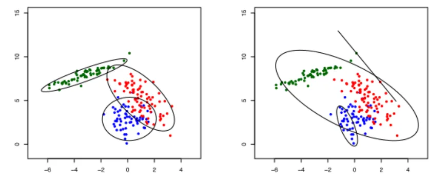
– Simdata 2:A second example is provided by considering a smaller subset (of size 100) drawn from the same set of parameters we considered before. Figure 2 shows the original data in panel a), a first classification based on the MLE ˆψ in panel b), a second classification based on a local maximum ψ∗ in panel c), and finally a third classification based on a spurious
max-imizer (in panel d), where one component is overfitted to a set composed by 4 data points).
−6 −4 −2 0 2 4
05
1
0
−6 −4 −2 0 2 4
05
1
0
a) b)
−6 −4 −2 0 2 4
05
1
0
−6 −4 −2 0 2 4
05
1
0
c) d)
Fig. 2 Simdata 2:a) original data; b) classification based on the MLE ˆψ; c) classification
based on a local maximumψ∗; d) classification based on a spurious solution.
one for the “true” mixture parameters. McLachlan and Peel (2000) offers a 11 pages analysis, applied to different synthetic and benchmark datasets, to show how the issue arises. In particular, the well-known Iris data set is analyzed to evaluate whether the “virginica” species should be split into two subspecies or not. To provide hints for distinguishing spurious from useful solutions, 15 possible local maxima were considered, together with different quantities sum-marizing clusters as the size of the smallest cluster, the determinants of the scatter matrices, the value of the smallest eigenvalue, and the intercomponent mean distances.
The likelihood estimate ψ must be one of the roots of the equation
∂L(ψ)
∂ψ =0. (11)
In a quite general framework (i.e. not restricted to mixture distributions), Cram´er (1946) showed that a unique consistent root exists for the equation (11) in the univariate case under certain conditions. The proof has been extended to the multivariate case by Chanda (1954), with a corrected version of Theorem 2 there provided by Tarone and Gruenhage (1975, 1979). See also Kiefer (1978) and Redner and Walker (1984).
Theorem 1 (Redner and Walker, 1984) Letp(x;ψ)be a probability den-sity function depending on some parameter ψ and assume we are provided with a sample {x1, . . . ,xN} drawn from p(x;ψ). Let ψ0 be the true value of the parameter ψ and exists at some point in the parameter space Ψ. Then, given the existence of, and certain boundedness conditions on, derivatives of the mixture density p(x;ψ), of orders up to 3, there exists a unique consis-tent estimatorψN corresponding to a solution of the likelihood equation (11). Further,√N(ψN−ψ0)is asymptotically normally distributed with mean zero and covariance I−1(ψ0), where I(ψ0)is the Fisher information matrix.
In the following, by maximum likelihood estimate (MLE), we shall mean such a point ofΨ and it will be denoted by ˆψ.
3 Constrained formulations of maximum-likelihood estimation The MLE ˆψ is usually computed by means of suitable optimization proce-dures which generate a sequence of estimates {ψ(r)}r – starting from some
initial guessψ(0) – so that the corresponding sequence {L(ψ(r))}r is not
de-creasing. To this end, the EM algorithm is usually implemented for parameter estimation in mixture modeling, see e.g. McLachlan and Krishnan (2008b). However, the convergence towards ˆψ is not guaranteed because of the nu-merical issues associated to the maximization of the log-likelihood function
3.1 Hathaway’s approach
The idea of a constrained estimation became popular due to Hathaway (1985), in the framework of Gaussian mixtures. In the univariate case, the Gaussian mixture has density
p(x;ψ) =π1φ(x;µ1, σ21) +· · ·+πGφ(x;µG, σ2G), (12)
whereψ∈Ψ andΨis the parameter space
Ψ={(π1, . . . , πG, µ1, . . . , µG, σ1, . . . , σG)∈R3G :
π1+· · ·+πG= 1, πg>0, σg>0 forg= 1, . . . , G}. (13)
For somec >0, letΨc be the subset ofΨsuch that σg2≥cσ2j forg=j, i.e.,
such that
min
g=j
σg2
σj2
≥c > 0. (14)
Hathaway (1985) pointed out that the first mention of constraints like (14) is found in Dennis (1981) who, in turn, gives credit to Beale and Thompson (oral communication). For this reason, Gallegos and Ritter (2009) called them the Hathaway-Dennis-Beale-Thompson (HDBT) constraints.
The following result states that the constraint (14) yields an optimization problem having a global solution in a constrained parameter space with no singularities and at least with a smaller number of local maxima.
Theorem 2 (Hathaway, 1985) Let X = {x1, . . . , xN} be a sample drawn with law (12) containing at least G+ 1 distinct points. Then for c ∈ (0,1]
there exists a constrained global maximizer ofL(ψ)over the setΨc defined by
(14).
Moreover, also strong consistency of the constrained estimator has been proven in Hathaway (1985), by applying existing maximum-likelihood theory due to Kiefer and Wolfowitz (1956). From a practical point of view, Hath-away (1996) provides an algorithm for building a consistent estimator under a slightly different kind of constraints:
σ2g
σg2+1
≥c for all g= 1, . . . , G−1 and σ
2 G
σ21 ≥c > 0.
Strong consistency is shown in Hathaway (1985) for the univariate case by applying existing maximum-likelihood theory due to Kiefer and Wolfowitz (1956), see Theorems 3.1 and 3.2.
Consider now the multivariate Gaussian mixture
p(x;ψ) =π1φ(x;µ1,Σ1) +· · ·+πG(x;µG,ΣG) (15)
whereψ∈Ψ with
Ψ={(π1, . . . , πG,µ1, . . . ,µG,Σ1, . . . ,ΣG)∈RG[1+d+(d
2+d)/2]
To generalize results in themultivariate case, Hathaway (1985) states only the following sentence in the concluding remarks: “For a mixture ofG d-variate normals, constraining all characteristic roots ofΣgΣ−j1 (1 ≤g =j ≤G) to
be greater than or equal to some minimum value c >0 (satisfied by the true parameter) lead to a constrained (global) maximum-likelihood formulation”. Being just a brief statement, this sentence motivated research summarized in Section 3.3.
3.2 Constraints on the determinants of the covariance matrices
The natural multivariate generalization of (14) appears to be a constraint on the ratio of the component generalized variances, i.e. of the determinants of the covariance matrices, which are required not to be too disparate:
min
g=j |Σg| |Σj|
= min
g=j|ΣgΣ −1
j | ≥c , (17)
for somec >0. The maximization of the loglikelihood function (7) under the constraint (17) is discussed in McLachlan and Peel (2000, Section 3.9.1).
Recalling that the volume is proportional to the square root of the deter-minant, we see that this type of constraint limits the relative volumes of the aforementioned equidensity ellipsoids, but not the cluster shapes. The use of this constraint is particularly advisable when affine equivariance is required. Constraints (17) have been implemented in the R package tclust, see Fritz
et al.(2012).
Finally, we recall that in the framework of the trimming approach to robust modeling, Gallegos (2002) implicitly assumed the stronger condition |Σ1| =
|Σ2|=· · ·=|ΣG|.
3.3 Constraints on the eigenvalues of the covariance matrices
As we recalled in Section 3.1, Hathaway (1985) proposed the constraint
min
g=j λ(ΣgΣ −1
j )≥c > 0, (18)
stating that it leads to a constrained (global) maximum-likelihood formulation, without any further development. The constantcin (18) is still referred to as the HDBT constant.
It is worth to note that, while this bound can be easily checked, as far as we know, it cannot be directly implemented in optimization procedures like the EM algorithm, where the estimates are iteratively updated. To this end, different approaches have been pursued.
Proposition 3 (Ingrassia, 2004) LetA,Btwod×dsymmetric and positive definite matrices. Then we have:
λmax(AB−1)≤ λmax(A)
λmin(B) (19)
λmin(AB−1)≥ λmin(A)
λmax(B) (20)
where λmin(M) and λmax(M) are respectively the smallest and the largest eigenvalue of the matrix M.
The proof is based on the properties of the spectral norm A 2of a matrix A. Denote byλig =λi(Σg) the ith eigenvalue of the gth covariance matrix.
For givena, b >0, such thata/b≥c, wherecsatisfies the relation (18), assume that the eigenvalues of the covariance matricesΣg satisfy the constraints:
a≤λi(Σg)≤b i= 1, . . . , d g= 1, . . . , G. (21)
Then for any pair of covariance matricesΣg,Σj, the inequality (20) yields:
λmin(ΣgΣ−j1)≥
λmin(Σg)
λmax(Σj) ≥
a
b ≥c >0, 1≤g=j≤G,
assuring that
λ∗min
λ∗max ≥c (22)
where
λ∗min= min
g=1,...,Gi=1min,...,dλi(Σg) (23)
λ∗max= max
g=1,...,Gi=1max,...,dλi(Σg). (24)
Finally, according to (21), we introduce the following constrained parame-ter space
Ψa,b =
(π1, . . . , πG,µ1, . . . ,µG,Σ1, . . . ,ΣG)∈RG[1+d+(d
2+d)/2]
:
G
g=1
πg= 1, πg>0, a≤λig≤b, g= 1, . . . , G , i= 1, . . . , d
. (25)
Theorem 4 Let X = {x1, . . . ,xN} be a sample drawn from a multivariate Gaussian mixture containing at leastG+ddistinct points. Then, for any pos-itive real numbersa, b, witha < b, there exists a constrained global maximizer of L(ψ)over the setΨa,b defined by (25).
Proof. To maximizeL(ψ) means to jointly maximize|Σg|−1/2 and minimize
the argument of the exponential, i.e. (xn−µg)Σg−1(xn−µg), for each g =
1, . . . , G. Hence, firstly we will show that, for a givenΣg, the mean vectorµg
has to lie in a compact subset in Rd. Let C be the convex hull of X, i.e. the
intersection of all convex sets containing the N points, given by
C(X) =
N
n=1
unxn| N
n=1
un= 1, un≥0
. (26)
Suppose now that ¯ψ ∈Ψa,b satisfiesµg ∈/ C(X). Then L( ¯ψ)≤ L(ψ∗) where
ψ∗∈Ψa,b is obtained from ¯ψ by changing thegth mean component toµ∗ g =
αµg for some α ∈ (0,1) (i.e., along the line joining 0 and µg) such that
µ∗
g∈C(X).
Let us set S ={ψ ∈Ψa,b|µg ∈C(X); 0< a≤λi(Σg)≤b <+∞ g =
1, . . . , G}. Then, it follows that
sup
ψ∈Ψa,b
L(ψ) = sup
ψ∈S L(ψ).
By the compactness ofSand the continuity ofL(ψ), there exists a parameter ˆ
ψ∈Ψa,b satisfying
L( ˆψ) = sup
ψ∈Ψa,b
L(ψ) = sup
ψ∈SL(ψ)
by Weierstrass’ theorem.
The above recipes obviously require some a priori information on the co-variance structure of the mixture throughout the bounds a and b in such a way thatΨa,b contains the maximum likelihood estimate ˆψintroduced at the
end of Section 2 and, at least, a reduced number of spurious maximizers. When we lack such information, this position introduce subjectivity and this is a drawback. Hence, in Ingrassia and Rocci (2007), a weaker constraint is directly imposed on the ratio a/b, setting a/b ≥ c, and using a suitable parameterization forΣg. Let us rewrite them as Σg =η2Ωg (g = 1, . . . , G),
where minigλi(Ωg) = 1 and impose the constraints
1≤λi(Ωg)≤
1
c, (27)
fori= 1, . . . , d andg = 1, . . . , G. The constraints (27) are weaker than (21), in fact if (21) are satisfied and we setη2= minigλi(Σg) and Ωg =Ση2j then,
by noting thatλi(Ωg) =η−2λi(Σg), we obtain
1≤λi(Ωg)≤
b a ≤
Constraints (27), in turn, are stronger than (18). In fact, if the former are satisfied then
λmin(ΣgΣ−j1)≥
λmin(Σg)
λmax(Σj)
= λmin(Ωg) λmax(Ωj) ≥
c, 1≤g=j≤G .
Other similar constraints are proposed in Ingrassia and Rocci (2007).
The constraints (21) (as well as the constraints (27) and others of the same kind) can be implemented quite easily in the EM algorithm, using the spectral decomposition theorem. It is well known that any symmetric matrixAcan be decomposed as:
A=ΓΛΓ (28)
whereΛis the diagonal matrix of the eigenvalues ofA, andΓis an orthogonal matrix whose columns are standardized eigenvectors. Based on the formula (28), at ther-th iteration of the EM algorithm we can build an estimateΣ(gr)
of the covariance matrixΣg such that the eigenvaluesλ( r)
ig =λi(Σ(gr)) satisfy
the constraints (21), by setting:
λ(igr)= min
b,max
a, l(igr)
(29)
where l(igr) is the update of λi(Σg) computed in the unconstrained M-step
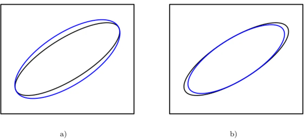
of the EM algorithm. The behaviour of (29) is illustrated in Figure 3. These constraints have been implemented in Ingrassia (2004), Ingrassia and Rocci (2007) and in Greselin and Ingrassia (2010), both for mixtures of multivariate Gaussian distributions and mixtures of multivariatetdistributions. We remark that the approach (29) is not scale invariant.
An important issue concerns themonotonicity of the constrained EM al-gorithms described above. To this end, the following results hold.
Theorem 5 (Ingrassia and Rocci, 2007) LetL(ψ)be the loglikelihood func-tion for a mixture of elliptical distribufunc-tions (2), given a sample X of size N. Denote by {ψ(r)}
r the sequence of the estimates generated by the EM algo-rithm, whereψ(r)∈Ψ
a,b, forr≥1. Then, the resulting sequence of the loglike-lihood values{L(ψ(r))}
r is not decreasing, once the initial guess ψ(0)∈Ψa,b.
The proof relies on the following inequality, due to Theobald (1975, 1976). Let A,Bbe two real symmetricd×dmatrices and letΛA,ΛBbe the corresponding
diagonal matrices of the eigenvalues. Then, it results tr(AB−1)≥tr(ΛAΛ−B1).
We remark that, even if the constraint (29) leads to a monotone EM algo-rithm, the choice ofa, bis quite critical.
3.4 Equivariant constraints based on eigenvalues of the covariance matrices
Very recently, Rocciet al.(2017) proposed a generalization of the constraint (21) that enforces the equivariance with respect to linear affine transformation of the data. LetAbe ad×dnon singular matrix and b∈Rd and consider
a) b)
Fig. 3 Results of enforcing constraints (29) on the eigenvalues of the covariance matrix at
r-th step: a) Iflig(r)< a(the covariance ellipse in dashed black) then the lowest eigenvalue should be forced to be equal to constant a(the covariance ellipse in blue). On the other hand, in b), ifl(igr) > b(covariance ellipse in dashed black), then the greatest eigenvalue should be shrunk to constantb(the covariance ellipse in blue).
We easily see that
φ(x;µ,Σ) =|A|φ(x∗;µ∗,Σ∗) (31) where µ∗ =Aµ+bandΣ∗ =AΣA. If we consider Gaussian mixtures, it can be easily proven that the relation between the loglikelihood of the original data (7) and the loglikelihood of the transformed data is given by
L(ψ) =Nlog|A|+L(ψ∗) (32)
where L(ψ∗) =Nn=1logGg=1πgφ(x∗n;µ∗g,Σ∗g)
is the loglikelihood based on the transformed data. Moreover, it can be proved that the classification of units, based on the maximum posterior probabilities, is invariant under this group of linear affine transformations.
It can be easily shown that constraints of kind (21) do not preserve the equivariance and this implies that the clustering depends on the choice of the matrix A in (30). In particular, constraints of kind (21) are sensitive to change in the units of data measurement. To overcome this drawback, Rocci
et al.(2017) recently proposed to generalize the constraint (21) by considering
a≤λi(ΣgΞ−1)≤b (33)
this constraint implies (18), indeed we have
λmin(ΣgΣ−j1)≥λmin(ΣgΞ−1)λmin(ΞΣ−j1) =
λmin(ΣgΞ−1)
λmax(ΞΣ−j1) ≥ a
b ≥c.
The constraint (33) is shown to lead to an affine equivariant maximum likeli-hood function. Rocciet al.(2017) discuss also some data-driven choices forΞ andcand propose an algorithm for maximizing (7) under the constraint (33).
3.5 Constraints on the ratio between maximum and minimum eigenvalues of the covariance matrices
A fully developed approach based on controlling the ratio between the max-imum and the minmax-imum eigenvalues of the groups scatter matrices has been proposed in Garc´ıa-Escuderoet al.(2015). It is based on the robust classifica-tion framework previously developed by the same authors in Garc´ıa-Escudero
et al.(2008), where a proportion of contaminating data was also discarded, to guarantee the robustness of the estimation.
The crucial feature introduced in Fritzet al.(2012) is that the optimum of the eigenvalues in the constrained space is obtained in closed form at each step of the EM algorithm. All previous attempts only offered approximations for it. For instance, Garc´ıa-Escuderoet al.(2008) was based on the Dykstra (1983) algorithm. Ingrassia and Rocci (2007) and Greselin and Ingrassia (2010) were just based on truncating the scatter matrices eigenvalues to assure monotonic-ity of the likelihood throughout (29). They implemented the constraint
λ∗max λ∗min ≤c
(34)
wherec≥1 is a fixed constant, andλ∗min andλ∗max have been defined in (23) and (24), respectively. Note that the constraint (34) is equivalent to the one introduced in (22), withc = 1/c.
Let Ψ∗c be the set of mixture parameters obeying that eigenvalues ratio constraint for constantc= 1/c≥1.
We take the opportunity of discussing in more depth this type of constraints here. They simultaneously control differences between groups and departure for sphericity. Note that the relative length of the equidensity ellipsoids axes, based onφ(·;µg, Σg), is forced to be smaller than√c, see Figure 4. The smaller
c, the more similarly scattered and spherical the mixture components are. For instance, for c = 1 these ellipsoids reduce to balls with the same radius, so extending k-means, in the sense of allowing different component weights.
l1, 1
l1, 2
l2, 1
l2, 2
Fig. 4 If{lh,g}denotes the length of the semi-axes of the equidensity ellipsoids based on
the normal densityφ(·;µg,Σg) forh= 1,2 andg= 1,2, we set max{lh,g}/min{lh,g} ≤√c by (34).
thatP is completely inappropriate for a mixture fitting approach by requiring that the distributionP is not concentrated onGpoints.
Proposition 6 (Garc´ıa-Escuderoet al., 2015) If P is not concentrated onGpoints andEP[ · 2]<∞, then there exists some ψ∈Ψ∗c such that the maximum of (9)under the constraint (34)is achieved.
The following consistency result also holds under similar assumptions.
Proposition 7 (Garc´ıa-Escuderoet al., 2015) Let us assume that P is not concentrated on G points and EP[ · 2] < ∞, and let ψ0 be the unique maximum of (9) under the constraint (34). If ψN ∈ Ψ∗c denotes a sample version of the estimator based on the empirical measurePN, then ψN →ψ0 almost surely, asN → ∞.
The consistency result presented in Garc´ıa-Escuderoet al.(2008) needed an absolutely continuous distributionP with strictly positive density function (in the boundary of the set including the non-trimmed part of the distribu-tion). This condition was needed due to the “trimming” approach considered by the TCLUST methodology. On the other hand, Propositions 6 and 7 do not longer need this assumption, it instead requires the finite second order moments hypothesis to control the tails of the mixture components.
are involved. Results in Hennig (2004), Ingrassia (2004), Ingrassia and Rocci (2007) and Greselin and Ingrassia (2010) may be seen as first steps toward the theoretical results presented in Garc´ıa-Escuderoet al. (2015).
The constraints (34) have been firstly implemented in a Classification EM algorithm by solving several complex optimization problems at each iteration of the algorithm, through Dykstra’s algorithm (Dykstra, 1983), to minimize a multivariate function on Gd parameters under Gd(Gd−1)/2 linear con-straints. This original problem is computationally expensive, even for moder-ately high values ofGorp. After introducing an efficient algorithm for solving the constrained maximization of the M step (Fritz et al., 2013), besides the singular-value decompositions of the covariance matrices, only the evaluation of a univariate function 2Gd+1 times is needed in the new M-step, with afford-able computing time with respect to standard EM algorithms. More recently, the versions for constrained mixture estimation (Garc´ıa-Escuderoet al., 2015) and robust mixture modeling (Garc´ıa-Escudero et al., 2014) have also been developed by the same authors.
It is important to note that the estimator in Garc´ıa-Escuderoet al.(2015) is well defined as a maximum of the likelihood in the constrained space. The proposed algorithm tries to find this maximum by applying the constrained EM algorithm with multiple random initializations. Proposition 7 shows that the solution of the sample problem converges to the solution of the population one. The consistency result in Redner and Walker (1984) states that there is a sequence of local maxima of the likelihood converging to the optimum. Un-fortunately, it does not provide a constructive way to choose the right optimal local maximum, for a fixed sample problem of sizeN, to obtain the consistent sequence.
We have seen that constraining the ratio between the scatter matrices eigenvalues to be smaller than a fixed in advance constant c leads to an approach with nice theoretical properties (existence and consistency results) and a feasible algorithm for its practical implementation. Now we still may wonder on how to properly select the c constant. In Garc´ıa-Escudero et al.
3.6 Affine equivariant constraints on covariance matrices based on L¨owner partial ordering
A different kind of constraints on the eigenvalues of the covariance matrices has been considered in Gallegos and Ritter (2009), resorting to the L¨owner matrix ordering, in the framework of robust clustering. This approach is affine equivariant, as it can be easily seen.
Let A andB be symmetric matrices of equal size. We say that A is less than or equal to B w.r.t. L¨owner’s (or semi-definite) order, and we denote it by A B, if B−A is positive semi-definite. Analogously, if B−A is positive definite, then we will write A ≺ B. Puntanen et al. (2011) remark that the L¨owner matrix ordering is a surprisingly strong and useful property. In particular, we recall that ifAB, then it resultsλi(A)≤λi(B), implying
that trace(A)≤trace(B) and det(A)≤det(B).
To be more specific, Gallegos and Ritter (2009) constrained the scatter matrices to satisfy
cΣjΣg for every j =g= 1, . . . , G, (35)
wherec≥0 is the HDBT constant, introduced in (18). It can be proved that the constraint (35) can be equivalently written as
λ(Σ−1/2
j ΣgΣ−1 /2
j )≤c for every g, j= 1, . . . , G. (36)
Differently from the previous cases, the constraint (35) depends also on the orientation of the covariance matrices. To see it, let A be a positive definite matrix and B =VAV be its rotation, under some orthonormal matrix V. Then, in general,B−Ais not positive definite, i.e. A≺B. In Figure 5 the matrix A = diag(1,4) and some rotations ofA are considered according to the rotation matrix
Vθ=
cosθ−sinθ sinθ cosθ
For instance, let
Biπ/6=Viπ/6AViπ/6,
for i = 1,2,3. Different suitable values of constant c are required in order to ensure that cBiπ/6 A. In other words, the ordering depends not only
on the eigenvalues but also on the relative rotation between the ellipsoids of equidensity. The largest values ofc such that cBiπ/6 Aarec∗π/6 = 0.4802,
a)θ= 0,c0= 1 b)θ=π/6,c∗π/6= 0.4802
c)θ=π/3,c∗π/3= 0.2947 d)θ=π/2,c∗π/2= 0.2499
Fig. 5 The L¨owner order is related to the relative sizeand the rotation between ellipsoids
of equidensity. The blue ellipse in panel a) is comparable with the blue ellipses in panels b), c) and d). The relationcBθAholds forc≤c∗θ wherec∗θ are the indicated thresholds.
4 On the degeneracy in the maximum likelihood estimation
Convergence properties of the EM algorithm nearby stationary point has been investigated in many papers. See e.g. Boyles (1983), Wu (1983), Meng (1994) and Nettleton (1999). Here we consider convergence properties of the EM towards a solution containing degenerate components, as introduced in Sec-tion 2. Let {ψ(r)}
r be a sequence of the estimates ofψ provided by the EM
and let{L(ψ(r))}
rbe the corresponding sequence of the loglikelihood values.
Throughout this section, for simplicity, the superscript “−” will denote the estimation at iteration r and the superscript “+” denotes the estimation at iterationr+ 1.
The behaviour of the EM algorithm near degenerate components has been first investigated in Biernacki and Chr´etien (2003) for mixtures of univariate Gaussian distributions. In particular, they prove the existence of a domain of attraction leading the EM algorithm to degeneracy.
Consider the sequence of the estimates{ψ(r)}rprovided by the EM
−6 −4 −2 0 2 4
0
5
10
15
−6 −4 −2 0 2 4
0
5
10
15
Fig. 6 Example of degenerate components
distributions (12), whereψ(r)∈Ψ, withΨdefined in (13). Let us set
fng(r)=πg(r)φ(xn;µ(gr), σ(gr) 2
), (37)
and assume that, at the current iteration of the EM algorithm, the component g0 (1≤g0 ≤G) is close to degeneracy at the unitxn0 (1≤n0≤N). Such a
situation is equivalent to a high densityfn(r0)g0 of componentg0 at xn0 and to
small densitiesfng(r)0 at other unitsxn (n =n0) (this occurs with probability
one, assuming all individuals to be different with probability one). Afterwards, set the vector
v0=
1/fn0g0,{fng0}n=n0
. (38)
For a degenerate component, the Euclidean norm v0 is small. Finally, denote byv(0r)the value ofv0 evaluated at steprof the EM algorithm. An example of degenerate component is given in Figure 6.
In this framework, Biernacki and Chr´etien (2003) prove two results that we summarize below, see Theorems 8 and 9.
Theorem 8 (Biernacki and Chr´etien, 2003) There existsε >0such that if v0 ≤ε then v(0r) =o v0 with probability one.
The proof follows from the Taylor expansions for parameters πg+0, µ+g0 and
σg2+0 . This results states that, if v0 is small enough, than the EM mapping is
contracting and, therefore, EM is convergent and its fixed point is degenerated The second results concerns the speed towards degeneracy.
Theorem 9 (Biernacki and Chr´etien, 2003) There exists ε > 0, α > 0
andβ >0 such that if v0 ≤εthen, with probability one
σg2+0 ≤α
exp(−β/σg20−)
σ2g−0
The proof follows again from the Taylor expansions. In particular, this results establishes that the variance of a degenerated component tends to zero with an exponential rate. Since the likelihood tends to infinity as fast as the inverse of the standard deviation, the divergence of the likelihood is exponential too. These results have been extended to the multivariate case in Ingrassia and Rocci (2011). In this case, a degenerate solutions occurs at some subset ofX containingq ≤d points. Thus, let Dbe a subset of {1,2, . . . , N} containing q≤dunits and consider the vector
v0=
{1/fng0}n∈D,{fng0}n∈D
(40)
which generalizes (38) in the multivariate setting. The following result extends Theorem 9 to the multivariate case.
Theorem 10 (Ingrassia and Rocci, 2011) Let g0 be a degenerate compo-nent of the mixture (3)), with 1≤g0≤G. LetΣ(gm0+1) be the estimate of the
covariance matrix Σj0 at iteration m+ 1∈N. There existε >0 andβ > 0 such that if v0 ≤εthen
λmin(Σ+g0)<
δ [λmin(Σ−g0)]d/2
exp
− β
4λmin(Σ−g0)
+ o||v0||. (41) The proof follows again from arguments based on the Taylor expansion.
The relation (41) suggests that, near degeneracy, the smallest eigenvalue decreases very fast. Based on this result, in Ingrassia and Rocci (2011) is conjectured that such bad behavior should be prevented by bounding the eigenvalues variations between two consecutive iterations. Thus, the idea is to control the speed of variation of both the smallest and the largest eigenvalues at each iteration and the following constraints have been proposed
λmin(Σ−j )/ϑa≤λ+ij ≤ϑbλmax(Σ−j), (42)
withϑa, ϑb>1 and thus from (42) we get
λ(ijm+1)= min
ϑbλmax(Σ( m) j ),max
λmin(Σ(jm))/ϑa, l( m+1) ij
. (43)
We refer to such constraints as “dynamic constraints” to point out that the bound on the eigenvalue at the current iteration depends on the value of the eigenvalue computed at the previous step of the algorithm. On the contrary, we shall refer to the type of constraints like in (21) as “static” because the interval remains fixed during the whole computation.
A monotone algorithm implementing (42) can be easily derived by us-ing the constrained EM algorithm of Ingrassia and Rocci (2007) previously described. We remark that this implementation does not lead to an EM al-gorithm, because in the “M-step” the complete log-likelihood function is not necessarily maximized. However, by noting that at iterationm+1 the complete log-likelihood is increased by every update ofλij lying in the interval
[min(λmij, l (m+1)
ij ),max(λ m ij, l
in the M-step the complete log-likelihood is always increased. This kind of algorithm, where the complete log-likelihood is increased instead of maximized, has been referred to asgeneralizedEM in Dempster et al.(1977).
We point out that such constraints have a different background with respect to (21), (27) and others proposed in Ingrassia and Rocci (2007). The latter are based on a constrained formulation of the likelihood function for mixture models; the constraints proposed here are in some sense of an algorithmic type being based on the convergence properties of the EM algorithm.
Our results highlighted that, in some way, the convergence of the EM algo-rithm to some spurious maximum is also due to the properties of the algoalgo-rithm itself. Indeed, since in the near degeneracy case the covariance matrices con-verge at exponential rate toward singularity, this implies that in such cases such a covariance matrix could model some spurious small group of data quite quickly and this amounts to an increase in the probability of the algorithm to get stuck into some spurious maximum.
In general, dynamic constraints performed always at least as good as the unconstrained EM algorithm and good performances were attained when both bounds on the variation of the eigenvalues were implemented.
5 Gaussian parsimonious clustering models
In literature, intermediate component covariance matrices lying between ho-moscedasticity and heteroscedasticity, have been proposed by Banfield and Raftery (1993) and Celeux and Govaert (1995). They proposed a general framework for geometric cross-cluster constraints in multivariate normal mix-tures by parameterizing covariance matrices through eigenvalue decomposition in the form
Σg=λgDgAgDg g= 1, . . . , G (44)
where Dg is the orthogonal matrix of the eigenvectors ofΣg, describing the
scatterorientation,Ag is a scaled (|Ag|= 1) diagonal matrix whose elements
are proportional to the eigenvalues ofΣgin decreasing order, giving theshape,
and λg is an associated constant of proportionality, related to the volume of
the clusters, which is proportional to λd/g 2 = |Σg|1/2. The idea is to treat
λg,Dg and Ag as independent sets of parameters and either constrain them
to be the same for each cluster or allow them to vary among clusters, see Table 1. In a quite different context, similar ideas have been introduced in Greselin
et al.(2011).
Hence, we allow the volumes, the shapes and the orientations of clusters to vary or to be equal between clusters. Variations on assumptions on the parametersλg,Dg and Ag (g = 1, . . . , G) lead to fourteen general models of
interest, plus two models for the univariate case. For instance, we can assume different volumes and keep the shapes and orientations equal by requiring that Ag = A (A unknown) and Dg = D (D unknown) for g = 1, . . . , G.
Model ID Model Distribution Volume Shape Orientation # parameters
E univariate equal 1
V univariate variable G
EII [λI] spherical equal equal NA α+ 1 VII [λgI] spherical variable equal NA α+d EII [λA] diagonal equal equal coordinate axes α+d VEI [λgA] diagonal variable equal coordinate axes α+d+G−1 EVI [λAg] diagonal equal variable coordinate axes α+dG−G+ 1 VVI [λgAg] diagonal variable variable coordinate axes α+dG EEE [λDAD] ellipsoidal equal equal equal α+β VEE [λgDAD] ellipsoidal variable equal equal α+β+G−1 EVE [λDAgD] ellipsoidal equal variable equal α+β+ (G−1)(d−1) VVE [λgDAgD] ellipsoidal variable variable equal α+β+ (G−1)d EEV [λDgADg] ellipsoidal equal equal variable α+Gβ−(G−1)d
VEV [λgDgADg] ellipsoidal variable equal variable α+Gβ−(G−1)(d−1) EVV [λDgAgDg] ellipsoidal equal variable variable α+Gβ−(G−1)
VVV [λgDgAgDg] ellipsoidal variable variable variable α+Gβ
Table 1 Parameterizations of the covariance matrixΣg. We haveα=Gdin the restricted
case (equal weights,πg= 1/G) andα=Gd+G−1 in the unrestricted case.βdenotes the number of parameters of each covariance matrix, i.e.β=d(d+ 1)/2.
EEE VEE EVE EEV
VVE VEV EVV VVV
Fig. 7 Example of covariance matrices having different patterns according to Table 1.
[λDgADg] means that we consider the mixture model with equal volumesλ,
equal shapes A and different orientations Dg. All these models can be
esti-mated by the MCLUST software (Fraley and Raftery, 1999, 2003, 2006; Fraley
This approach has been extended to multivariate t-distributions by An-drewset al. (2011).
We see that all models with equal volume and equal shape offer a good alternative when looking at covariance constraints to avoid singularities and reduce spurious solutions. For the other cases, “NA” values could appear in MCLUST results, due to failure in the EM computations caused by singu-larity and/or shrinking components, meaning that a particular model cannot be estimated. Hence a constraint on the eigenvalues is still needed, and the function emControlhas been added to MCLUST.
6 Mixtures of factor analyzers
The general Gaussian mixture model (3) is a highly parameterized model, with a total of (G−1) +G[d+d(d+ 1)/2] parameters. Looking for parsi-mony, it is of interest to develop some methods for reducing the covariance matrices parametrizationΣg, requiringGd(d+ 1)/2 parameters. To this
pur-pose, Ghahramani and Hinton (1997) and Tipping and Bishop (1999) proposed Gaussian Mixtures of Factor Analyzers (MFA), able to explain multivariate observations, by explicitly modeling correlations between variables.
This approach postulates a finite mixture of linear sub-models for the dis-tribution of the full observation vector X, given the (unobservable) factors U. Hence, it provides local dimensionality reduction by assuming that the distribution of the observationXn is given by
Xn=µg+ΛgUng+eng g= 1, . . . , G, n= 1, . . . , N, (45)
with probabilityπg, whereΛgis a d×qmatrix offactor loadings, thefactors
U1g, . . . ,UN g areN(0,Iq) distributed independently of theerrors eng, which
are N(0,Ψg) distributed, andΨg is a d×ddiagonal matrix (g = 1, . . . , G).
The diagonality of Ψg is one of the key assumptions of factor analysis: the
observed variables are independent given the factors.
Note that the factor variables Ung model correlations between the
ele-ments of Xn, while the eng variables account for independent noise for Xn.
We suppose thatq < d, which means thatq unobservable factors are jointly explaining the dobservable features of the statistical units. Under these as-sumptions, the mixture of factor analyzers model is given by (3), where the g-th component-covariance matrixΣg has the specific form
Σg =ΛgΛg+Ψg (g= 1, . . . , G). (46)
The parameter vectorθ =θM F A(d, q, G) now consists of the elements of the
component meansµg, theΛg, and theΨg, along with the mixing proportions
πg (g= 1, . . . , G−1), on puttingπG= 1−
G−1
g=1 πg. Note that, in the case of
q >1, there is an infinity of choices forΛg, since model (45) is still satisfied
if we replaceΛg by ΛgH, where H is any orthogonal matrix of order q. As
q(q−1)/2 constraints are needed forΛg to be uniquely defined, the number
Model ID Loading matrixΛg Error varianceΨg IsotropicΨg=ψgI # parameters
CCC Constrained Constrained Constrained [pq−q(q−1)/2] + 1 CCU Constrained Constrained Unconstrained [pq−q(q−1)/2] +p CUC Constrained Unconstrained Constrained [pq−q(q−1)/2] +G CUU Constrained Unconstrained Unconstrained [pq−q(q−1)/2] +Gp UCC Unconstrained Constrained Constrained G[pq−q(q−1)/2] + 1 UCU Unconstrained Constrained Unconstrained G[pq−q(q−1)/2] +p UUC Unconstrained Unconstrained Constrained G[pq−q(q−1)/2] +G UUU Unconstrained Unconstrained Unconstrained G[pq−q(q−1)/2] +Gp
Table 2 Parsimonious covariance structures introduced for mixtures of factor analyzers.
Parameters in mixtures of factor analyzers are usually estimated according to the likelihood approach, based on the AECM algorithm (Meng and van Dyk, 1997). AECM is a variant of the EM procedure, where two E and conditional M steps are alternated, acting on a partition of the parameter space, particularly suitable for ML for Gaussian factors.
McNicholas and Murphy (2008) extended the idea of patterned covari-ance matrices to mixture of factor analyzers by considering constraints across groups on theΛg andΨgmatrices and on whether or notΨg=ψgIp. The full
range of possible constraints provides a class of eightparsimonious Gaussian mixture of factor analyzer models, which are given in Table 2. These models provide a unified modeling framework which includes the mixtures of prob-abilistic principal component analyzers and mixtures of factor of analyzers models as special cases. This approach has been extended in different direc-tions: Andrews and McNicholas (2011) generalized this family of models to multivariatetdistributions while Subediet al.(2013) and Subediet al.(2015) introduced their version for cluster-weighted models.
To discuss these models from their ability to deal with singularity and spu-rious solutions along the ML estimation, we observe that the error matrices are either “unconstrained isotropic”Ψg=ψgIwith differentψgfor each
com-ponent, or “constrained isotropic”, sayΨg =Ψ=ψI. This parameterization
choice leads the covariance matricesΣg=ΛgΛg+Ψg far from singularities.
In a different approach, Greselin and Ingrassia (2015) constraints of type (21) have been proposed for mixtures of factor analyzers. Due to the structure of the covariance matrixΣg given in (46), bound in (21) yields
a≤λ(ΛgΛg+Ψg)≤b, g= 1, . . . , G . (47)
Concerning the squared×dmatrix ΛgΛg (g = 1, . . . , G), we can get its
eigenvalue decomposition, i.e. we can findΛg andΓg such that
ΛgΛg=Γg∆gΓg (48)
where Γg is the orthonormal matrix whose columns are the eigenvectors of
of ΛgΛg, sorted in non increasing order, i.e.δ1g ≥δ2g ≥. . . ≥δqg ≥0, and
δ(q+1)g=· · ·=δdg= 0.
Now, let us consider the singular value decomposition of thed×q rectan-gular matrixΛg, so givingΛg=UgDgVg, whereUgis ad×dunitary matrix
(i.e., such thatUgUg=Id) andDgis ad×qrectangular diagonal matrix with
qnonnegative real numbers on the diagonal, known assingular values, andVg
is a q×q unitary matrix. The dcolumns of U and theq columns of V are called theleft singular vectors and right singular vectors of Λg, respectively.
Now we have that
ΛgΛg= (UgDgVg)(VgDgUg) =UgDgIqDgUg=UgDgDgUg (49)
and equating (48) and (49) we getΓg=Ug and∆g=DgDg, that is
diag(δ1g, . . . , δqg) = diag(d21g, . . . , d2qg)., (50)
withd1g≥d2g≥ · · · ≥dqg≥0. In particular, it is known that only the firstq
values ofDg are non negative, and the remainingd−qterms are null.
Denoting now by ψig the i-th eigenvalue of Ψg, then constraint (47) is
satisfied when
d2ig+ψig≥a i= 1, . . . , d (51)
dig≤
b−ψig i= 1, . . . , q
ψig≤b i=q+ 1, . . . , d (52)
for g = 1, . . . , G. In particular, we remark that condition (51) reduces to ψig≥afori= (q+ 1), . . . , d.
The two-fold (eigenvalue and singular value) decomposition of theΛg
pre-sented above, suggests how to modify the EM algorithm in such a way that the eigenvalues of the covariancesΣg(forg= 1, . . . , G) are confined into suitable
ranges. Details are given in Greselin and Ingrassia (2015). Finally, we observe that only constraints onΨgare needed to discard singularities and to reduce
spurious maximizers, as it has been done in a robust approach for estimating Mixtures of Gaussian factors in Garc´ıa-Escuderoet al.(2016).
7 Concluding remarks
In the maximum likelihood approach for model based clustering and classifi-cation, based on mixtures of elliptical components, we have recalled here the need of considering a constrained parameter space for the covariance matrices, to yield a well posed optimization problem.
recent contributions in the literature that allows for milder conditions, and arriving to dynamic and/or affine equivariant constraints. We developed a detailed comparison of the advantages of each proposal, also in view of ob-taining a sound theoretical framework assuring existence and consistency to the obtained estimator.
Usually, the ML estimation is performed by using the EM algorithm. The latter is a powerful iterative process, leading deterministically to a specific solution, depending from the initial step. This makes the choice of the starting points a very delicate matter. Many efforts have been made in the literature to devise smart initialization methods, mainly to avoid convergence toward singularities or spurious solutions. We have seen that the constrained approach with a reasonable number of random initializations, on the other hand, yields to a reduced set of meaningful solutions. The researcher can devise among them the most convincing one, or the more interesting from the point of view of the obtained clustering, in view of his knowledge of the field of application. We argue that the clustering of a dataset should not be based solely on a single solution of the likelihood equation, but rather on the various solutions considered collectively and analyzed with care.
Finally, we discussed along the paper that the constrained approach in mixture modelling, beyond allowing a proper mathematical setting of the op-timization problem, at the same time provides stability to the obtained solu-tions.
As we stated in the introduction, the role of constrained estimation within robust statistical methods needs a longer discussion and will be the object of a further paper.
References
Andrews, J. L. and McNicholas, P. D. (2011). Extending mixtures of multi-variatet-factor analyzers. Statistics and Computing, 21, 361–373.
Andrews, J. L., McNicholas, P. D., and Subedi, S. (2011). Model-based classifi-cation via mixtures of multivariatet-distributions.Computational Statistics & Data Analysis, 55, 520–529.
Banfield, J. D. and Raftery, A. E. (1993). Model-based Gaussian and non-Gaussian clustering. Biometrics,49, 803–821.
Biernacki, C. and Chr´etien, S. (2003). Degeneracy in the maximum likeli-hood estimation of univariate gaussian mixtures with the EM. Statistics & Probability Letters,61, 373–382.
Boyles, R. A. (1983). On the convergence of the EM algorithm. Journal of the Royal Statistical Society B,45, 47–50.
Celeux, G. and Govaert, G. (1995). Gaussian parsimonious clustering models.
Pattern Recognition,28, 781–793.