Avoiding order reduction when integrating nonlinear Schrödinger equation with Strang method

Avoiding order reduction when integrating nonlinear

Schr¨

odinger equation with Strang method

B. Canoa,∗, N. Reguerab

a_{IMUVA, Departamento de Matem´atica Aplicada, Universidad de Valladolid, Facultad de}

Ciencias, Paseo de Bel´en 7, 47011 Valladolid, Spain.

b_{IMUVA, Departamento de Matem´aticas y Computaci´on, Escuela Polit´ecnica Superior,}

Universidad de Burgos, Avda. Cantabria, 09006 Burgos, Spain

Abstract

In this paper a technique is suggested to avoid order reduction when using Strang method to integrate nonlinear Schr¨odinger equation subject to time-dependent Dirichlet boundary conditions. The computational cost of this technique is negligible compared to that of the method itself, at least when the timestepsize is fixed. Moreover, a thorough error analysis is given as well as a modification of the technique which allows to conserve the symmetry of the method while retaining its second order.

Keywords: nonlinear Schr¨odinger equation, Strang method, symmetry, avoiding order reduction in time

1. Introduction

Exponential methods have been proved to be efficient in the numerical time integration of partial differential equations [16] although some times they show order reduction [4, 14]. Moreover, they have been usually used when considering homogeneous boundary conditions and the analysis has been performed under that assumption. Just some recent research [5, 6, 13] has been done to include non-homogeneous boundary conditions. Moreover, the techniques which are suggested there manage to avoid order reduction for both homogeneous and non-homogeneous boundary conditions. ([5] and [6] deal with Lawson and splitting methods whenintegrating linear problems and [13] with splitting methods for reaction-diffusion ones.)

In this paper, we will focus on the numerical integration of the nonlinear Schr¨odinger equation subject to Dirichlet boundary conditions. More precisely,

∗_{Corresponding author}

we search for the functionu∈C1([0, T], H2(Ω,C)) such that

ut(x, t) = i(∆u(x, t) +f(|u(x, t)|2)u(x, t)), t∈[0, T], x∈Ω,

u(x,0) = u0(x), x∈Ω,

∂u(t) = g(t), (1)

for a bounded domain Ω with smooth enough boundary ∂Ω, where ∂ is the Dirichlet trace operator in H2_{(Ω) [12], f is a smooth enough real function,}

u0 ∈H2(Ω,C) and g ∈ C1([0, T], H 3

2(∂Ω),C). (The precise conditions which are sufficient to assure the existence, uniqueness and well-posedness of such a solution, until a certain time T > 0, are non-trivial [7].) This problem has applications, for example, in ionospheric modification experiments [8].

For the time integration we will focus on Strang method, which is a sym-metric splitting method with classical order 2. The great advantage of using a splitting method for the nonlinear Schr¨odinger equation is that, as firstly noticed in[18], each part resulting from the decomposition

ut = i∆u, (2)

ut = if(|u|2)u, (3)

can be solved as linear, which leads to a very easy and cheap implementation. This comes from the fact that the solution of (3) leaves|u|invariant. (In fact, neglecting the error coming from the space discretization, both equations are exactly solvable.)

We shall offer a cheap technique to discretize (1) with Strang method in such a way that order reduction is completely avoided. The procedure is as cheap as that suggested, among other papers, in [1, 2, 3] to avoid order reduc-tion with Runge-Kutta type methods when integrating linear problems. Notice, however, that the technique here is different because the stages are not elliptic problems any more. Moreover, for Strang method, we will suggest a slight mod-ification of the procedure which even conserves symmetry while also avoiding order reduction.

The paper is structured as follows. Section 2 gives some preliminaries on the space discretization, Strang method and the drawbacks of dealing the problem in other different ways. Section 3 describes the technique which is suggested and gives the final formula to be implemented. In Section 4, the local error is studied with such a technique. Section 5 describes how to modify the method in order to conserve symmetry without losing order. Section 6 gives a thorough analysis of the global error ofthetime semidiscretization and, finally, in Section 7 some numerical experiments are shown which corroborate the previous results.

2. Preliminaries

and some other nodes on the boundary. More precisely, we will suppose that the discretization of the elliptic problem

∆u(x) = F(x), x∈Ω,

∂u = g,

whereF ∈L2_{(Ω,C) andg∈H}3

2(Ω,C),is done by solving the following system

Ah,0Rhu+Chg=PhF, (4)

where Ph is just the nodal projection on the interior grid nodes, Rhu is the

approximation to the values ofuin them,Ah,0is an invertible matrix which de-fines the discretization of the Laplacian with vanishing boundary conditions and

Chg is a vector which contains information on the values ofg in the boundary

grid nodes. We will consider the following hypotheses:

(H1) For a certain constant M, which is independent of h, and the discrete

L2_{-norm, the matricesA}

h,0 satisfy

||eitAh,0||

L2

h(Ω)≤M, t∈[0, T].

(H2) There exists a subspaceZ ofL2_{(Ω), such that, foru∈Z,} (a) ∆−₀1u∈Z, where ∆0= ∆|H2_(Ω)∩H1

0(Ω). (b) for someεh which is small withh,

∥Ah,0(Ph−Rh)u∥_L2

h(Ω)≤εh∥u∥Z. (5)

(That is, whenu ∈Z, this hypothesis means that, by doing (4), a consistent approximation of the Laplacian at the interior grid nodes is achieved.)

When the boundary conditions are homogeneous (g= 0), a space discretization of (1) leads to a system like

U_h′ = i(Ah,0Uh+f(|Uh|.2).Uh),

Uh(0) = Phu0, (6)

where . denotes pointwise vectorial multiplication. In this case of vanishing boundary conditions, no order reduction of the splitting method turns up. That can be observed in the numerical experiments and will also be shown in the subsequent analysis. (In fact, numerical results in [10] also confirm that when using a pseudospectral space discretization.) More precisely, when applying Strang method to (6), the following scheme turns up

U_hn+1=ek2iD2,n_ekiAh,0_ek2iD1,n_Un

h, (7)

whereUn

h approximatesu(·, tn) fortn=nk, withk the time stepsize,

D1,n= diag(f(|Uhn|.

2_{)), D}

2,n= diag(f(|Whn|.

2_{)), W}n

h =e

kiAh,0_ek2iD1,n_Un

h.

(i) If we first integrate (1) in space and then in time, a differential system like this turns up

U_h′(t) =iAh,0Uh(t) +iChg(t) +if(|Uh|.2).Uh, (8)

As we will describe in an example in Section 7, Chg(t) grows when h

diminishes. As Strang method applied to

U′=A1U+A2U+F(t) leads to

Un+1=ek2A1_ek2A2_(ek2A2_ek2A1_Un_+kF(t

n+

k

2)), when integrating (8),

U_hn+1=ek2iD2,n_ek2iAh,0_(ek2iAh,0_ek2iD1,n_Un

h +ikChg(tn+

k

2)), where

D1,n= diag(f(|Uhn|.

2_)),

D2,n= diag(f(|Whn|.

2_{)), W}n

h =e

k

2iAh,0_(ek2iAh,0_ek2iD1,n_Un

h +ikChg(tn+

k

2)). As we will see in Section 7, this leads to very poor results. The reason for that is thatChg take very big values whenh→0.

(ii) Another possibility which has been used in the literature for Runge-Kutta methodsonlinear problems [9] and splitting methods in diffusion-reaction problems [13] is to consider the solution of

∆z(x, t) = 0, x∈Ω,

∂z(t) = g(t), (9)

which is usually denoted as K∆(0)g(t). Then, making the difference with (1), the following initial boundary value problem with homogeneous boundary conditions turns up forw=u−z:

wt = i∆w−zt+if(|w+z|2)(w+z),

w(x,0) = u0(x)−z(x,0), x∈Ω, ∂w(t) = 0.

When decomposing the equation as

wt = i∆w+if(|z|2)z−zt, (10)

wt = if(|w+z|2)(w+z)−if(|z|2)z, (11)

has the following drawbacks: On the one hand, at each step, the calcu-lation of z through (9) is necessary. In the one-dimensional case, that just corresponds to a straight line and can be calculated analytically, as well aszt. However, in more dimensions, that would mean to solve two

elliptic problems at each step (one forzand another forztwith boundary

gt) when the boundary conditions and their derivatives depend on time.

On the other hand, the linear part (10) is not as directly solvable as (2) because a source term turns up now and what is more serious,|w+z|2_is not an invariant of (11) and therefore, that equation cannot be solved as if it were linear. Therefore, to integrate each of those parts, an additional time integrator would have to be used.

In the description and analysis of the procedure which is suggested here to avoid order reduction, we will useφ1(it∆0), φ2(it∆0) andφ3(it∆0), where

{φj}are the standard functionswhich areused in exponential methods [16]and

which are defined by

φj(tA) =

1

tj

∫ t

0

e(t−τ)A τ

j−1

(j−1)!dτ, j≥1. (12) Besides, the following is well-known to be satisfied [16]:

φ1(z) =e

z₋₁

z , φ2(z) =

φ1(z)−1

z , φ3(z) =

φ2(z)−1₂

z . (13)

These functions are bounded in the imaginary axis, which is the place where the eigenvalues ofit∆0lay, because ∆0is a selfadjoint operator inL2(Ω). Therefore,

eit∆0_{,φ1(it∆0),φ2(it∆0) andφ3(it∆0) are operators which are bounded inL}2 -norm for realt.

3. Description of the technique

In this section, we describe how to apply directly Strang exponential method to nonlinear Schr¨odinger equation with nonhomogeneous and possibly time-dependent Dirichlet boundary conditions in such a way that no order reduction is shown. The main idea is to integrate (1) firstly in time with suitable boundary values for the evolutionary partial differential equation and just then, to apply the space discretization to the problemsthat turn up.

3.1. Time semidiscretization

Starting from the numerical approximationun at timetn, for the time

inte-gration of (1), we firstly tackle the nonlinear part of the problem (3) and then solve

vn′(s) = if(|un|2)vn(s),

vn(0) = un,

considering its value ats=k/2. Secondly, in order to integrate the linear part (2), apart from an initial condition, we must also suggest a boundary. As we take as initial condition for this problemvn(k₂), for the boundary we consider

the first-order Taylor expansion ats= 0 of the searched functionwn satisfying

(2). More precisely,

wn(0) +sw′n(0) =vn(

k

2) +si∆vn(

k

2). (15)

On the other hand, in order to approximate this from the datawhich are given in the original problem (1), we will consider the following approximation for

vn(k₂), which comes from (14),

vn(

k

2)≈u(tn) +

k

2if(|u(tn)| 2_)u(t

n). (16)

Neglecting then terms of second order in k and s, when u ∈ H4_{(Ω) and}

f(|u|2_)u∈H2_{(Ω), we consider the solution of}

w_n′(x, s) = i∆wn(x, s), x∈Ω, (17)

wn(x,0) = vn(x,

k

2), x∈Ω,

∂wn(s) = ∂[u(tn) +

k

2if(|u(tn)| 2_)u(t

n) +si∆u(tn)],

= g(tn) +

k

2if(|g(tn)| 2_)g(t

n) +s[gt(tn)−if(|g(tn)|2)g(tn)].

Here (17) is understood in a generalized sense, in the same way thateit∆0_u 0 is understood when∂u0 ̸= 0 (see [6, 17]). Notice also that the last equality just comes from (1) considering that

∂[i∆u(tn)] =∂[ut(tn)−if(|u(tn)|2)u(tn)] =gt(tn)−if(|g(tn)|2)g(tn). (18)

Finally, evaluatingwn at s=kand integrating again the nonlinear part of the

problem (3), we get

z_n′(s) = if(|wn(k)|2)zn(s),

zn(0) = wn(k),

(19)

and then we consider

un+1=zn(

k

2). (20)

Remark 1. Notice that higher order terms of asymptotic expansion for the boundary ofwn(s)cannot be calculated from data since

vn(

k

2)≈u(tn) +

k

2if(|u(tn)| 2

)u(tn)−

k2

4 f(|u(tn)| 2

and then,

wn(0) +swn′(0) +

s2 2w

′′

n(0) =vn(

k

2) +si∆vn(

k

2)−

s2 2∆ 2_v n( k 2)

≈ u(tn) +

k

2if(|u(tn)| 2_)u(t

n)−

k2

4 f(|u(tn)| 2₎2_u(t

n)

+si∆u(tn)−

sk

2 ∆(f(|u(tn)| 2_)u(t

n))−

s2 2 ∆

2_u(t

n).

The trace of all these terms can be calculated except for ∂∆(f(|u(tn)|2)u(tn))

and∂∆2_u(t

n) at the same time. Notice that, from (18),

∂∆ut(tn) =−igtt(tn)−

d

dt[f(|g(t)|

2_)g(t)]|

t=tn, and from (1),

∂∆ut(tn) = i∂∆2u(tn) +i∂∆(f(|u(tn)|2)u(tn)).

Therefore, the sum of both terms can be calculated but not both of them sepa-rately.

3.2. Final formula after space discretization

When the space discretization is applied to (14),(17),(19), the following sys-tems turn up:

Vh,n′ (s) =idiag(f(|U n h|.

2

)Vh,n(s),

Vh,n(0) =Uhn,

Wh,n′ (s) =iAh,0Wh,n(s) +iCh[g(tn) +i

k

2f(|g(tn)| 2_)g(t

n))

+s[gt(tn)−if(|g(tn)|2)g(tn)]], (21)

Wh,n(0) =Vh,n(

k

2),

Z_h,n′ (s) =idiag(f(|Wh,n(k)|.2)Zh,n(s),

Zh,n(0) =Wh,n(k).

Notice that the solution of (21) ats=kis

Wh,n(k) =eikAh,0Vh,n(

k

2) +i

∫ k

0

ei(k−s)Ah,0_C

h

[

g(tn) +i

k

2f(|g(tn)| 2_)g(t

n)) +s[gt(tn)−if(|g(tn)|2)g(tn)]

] ds.

Therefore, the final formula for the implementation is the following. Starting fromU_h0=Phu0and denoting ˆVhn=Vh,n(k₂), ˆWhn=Wh,n(k) andUhn+1= ˆZ

n

Zh,n(k₂), from eachUhn we calculate U n+1

h in the following way:

ˆ

V_hn = eik2diag(f(|U

n h|.

2₎₎

U_hn,

ˆ

W_hn = eikAh,0_Vˆn

h +ikφ1(ikAh,0)Ch[g(tn) +i

k

2f(|g(tn)| 2_)g(t

n)]

+ik2φ2(ikAh,0)Ch[gt(tn)−if(|g(tn)|2)g(tn)],

U_hn+1 = eik2diag(f(|Wˆ

n h|.2))_Wˆn

h. (22)

Remark 2. Notice that the information on the boundary for the numerical inte-gration of (1) enters at each step through multiplication by matricesφ1(ikAh,0)

andφ2(ikAh,0). Although one could think that the computational cost of

calcu-lating each of those terms is similar to that of calcucalcu-latingeikAh,0_Vˆn

h, in practice

that is not the case for finite differences. In such a case, the vector Ch[·] has

many vanishing components and therefore just some columns ofφ1(ikAh,0)and

φ2(ikAh,0) are in fact necessary, which are of the order of the number of grid

nodes on the boundary, O(Nd−1_{) against O(N}d_{) for the total number of grid}

nodes where d is the dimension of the problem and N the average number of grid nodes in each direction. (Look at Section 7 for a particular example in one dimension in which just two columns are necessary.) For fixed stepsizek, once those columns are calculated at the very beginning, just a suitable linear com-bination of them must be added to the method at each step with this procedure.

4. Local error

4.1. Local error of the time discretization

In order to study the local error, we consider the valueun+1obtained in (20) starting fromun =u(tn) in (14).

Theorem 3. Let us assume that the solution uof (1) satisfies

(i) u∈C([0, T], H4_(Ω)),

(ii) f(|u|2_{)u∈C([0, T], H}2_(Ω))

(iii) f(|u|2₎2_{u∈C([0, T], L}2_(Ω)).

Then, when integrating (1) with Strang method using the technique (14),(17), (19),(20), the local errorρn+1=u(tn+1)−un+1 satisfies

∥ρn+1∥L2_(Ω)=O(k2).

Proof. Similarly to (14),(17),(19) and (20) and defining

wn,B(s) =u(tn) +i

k

2f(|u(tn)| 2_)u(t

we now consider the solutions of the following problems

v′_n(s) =if(|u(tn)|2)vn(s), vn(0) =u(tn),

w′_n(s) =i∆wn(s), wn(0) =vn(

k

2), ∂wn(s) =∂wn,B(s), (24)

z′_n(s) =if(|wn(k)|2)zn(s), zn(0) =wn(k),

Then,un+1_=z

n(k₂). Notice that

vn(

k

2) =e

ik

2f(|u(tn)|2)_u(t

n) =u(tn) +i

k

2f(|u(tn)| 2

)u(tn) +O(k2), (25)

where the residue is bounded inL2-norm because of hypothesis (iii). Then, for the differencewn(s)−wn,B(s), we have the following:

w′n(s)−w′n,B(s) = i∆wn(s)−i∆u(tn)

= i∆(wn(s)−wn,B(s)) +i∆(wn,B(s)−u(tn))

= i∆(wn(s)−wn,B(s))−

k

2∆(f(|u(tn)| 2_)u(t

n)−s∆2u(tn),

wn(0)−wn,B(0) = ei

k

2f(|u(tn)|2)_u(t

n)−u(tn)−i

k

2f(|u(tn)| 2_)u(t

n),

∂(w(s)−wn,B(s)) = 0.

Then, through a variation-of-constants formula,

wn(s)−wn,B(s) =eis∆0[ei

k

2f(|u(tn)| 2₎

u(tn)−u(tn)−i

k

2f(|u(tn)| 2_)u(t

n)]

−sk

2 φ1(is∆0)∆(f(|u(tn)| 2_)u(t

n))−s2φ2(is∆0)∆2u(tn) =O(k2).(26)

Because of the boundedness ofeik∆0_{, φ}

1(ik∆0) andφ2(ik∆0) and assumptions (i) and (ii), this implies that

wn(k) = u(tn) +

k

2if(|u(tn)| 2_)u(t

n) +ki∆u(tn) +O(k2),

which means that

un+1 = zn(

k

2) =e

ik

2f(|wn(k)|2)_w

n(k)

= u(tn) +kif(|u(tn)|2)u(tn) +ki∆u(tn) +O(k2) =u(tn+1) +O(k2).

4.2. Local error of the full discretization

In order to define the local error after full discretization, we consider

Uh,n+1=Zh,n(

k

2) =e

ik

2diag(f(|Wh,n(k)|.2))_W

whereWh,n(s) solves

W′_h,n(s) =iAh,0Wh,n(s)

+iCh[g(tn) +i

k

2f(|g(tn)| 2_)g(t

n)) +s[gt(tn)−if(|g(tn)|2)g(tn)]],

Wh,n(0) =Vh,n(

k

2) =e

ik

2diag(f(|Phu(tn)|.2)_P

hu(tn). (28)

Then,

Wh,n(k) =eikAh,0ei

k

2diag(f(|Phu(tn)|.2))_P

hu(tn)

+i

∫ k

0

ei(k−s)Ah,0_C

h

[

g(tn) +i

k

2f(|g(tn)| 2_)g(t

n)) +s[gt(tn)−if(|g(tn)|2)g(tn)]

] ds,

which can be inserted in (27).

We now define the local error att=tn as

ρh,n=Phu(tn)−Uh,n,

and study its behaviour in the following theorem.

Theorem 4. Under the same hypotheses of Theorem 3, assuming also thatf is locally Lipschitz continuous, that

u, f(|u|2)u,∆u∈C([0, T], Z), (29)

for the spaceZ which is defined in (H2) and hypotheses (H1)-(H2) for the space discretization, when integrating (1) with Strang method as described in (22),

∥ρh,n+1∥L2

h(Ω)=O(k

2_+kε

h), (30)

whereεh is that in (5).

Proof. Notice that

ρh,n+1=Phu(tn+1)−Uh,n+1=Phρn+1+ (Phun+1−Uh,n+1).

Then, from Theorem 3, the first term isO(k2_{). In order to bound the second} term, we take into account that

Phun+1−Uh,n+1=Phzn(

k

2)−Zh,n(

k

2) =Ph

[

eik2f(|wn(k)| 2₎

wn(k)

]

−eik2diag(f(|Wh,n(k)|. 2₎₎

Wh,n(k)

=eik2diag(Phf(|wn(k)|2))_P

hwn(k)−ei

k

2diag(f(|Wh,n(k)|.2))_W

h,n(k)

=[eik2diag(Phf(|wn(k)|2))−_eik2diag(f(|Wh,n(k)|.2))]_P

hwn(k)

+eik2diag(f(|Wh,n(k)|.2))_[P

Then, considering (23),(25) and (4),

Phw′n,B(s) = iPh∆u(tn)

= i[Ph∆wn,B(s)−i

k

2Ph∆(f(|u(tn)| 2_)u(t

n))−isPh∆2u(tn)]

= iAh,0Rhwn,B(s) +iCh∂wn,B(s) +

k

2Ph∆(f(|u(tn)| 2_)u(t

n))

+sPh∆2u(tn)

= iAh,0Phwn,B(s) +iCh∂wn,B(s) +iAh,0(Rh−Ph)wn,B(s)

+k

2Ph∆(f(|u(tn)| 2_)u(t

n)) +sPh∆2u(tn)

Phwn,B(0) = Phu(tn) +i

k

2f(|Phu(tn)|. 2_).P

hu(tn). (32)

Making now the difference with (28), we have that

Phw′n,B(s)−W

′

h,n(s) = iAh,0[Phwn,B(s)−Wh,n(s)] +iAh,0(Rh−Ph)wn,B(s)

+k

2Ph∆(f(|u(tn)| 2_)u(t

n)) +sPh∆2u(tn),

Phwn,B(0)−Wh,n(0) = Phu(tn) +i

k

2f(|Phu(tn)|. 2_).P

hu(tn)

−eik2diag(f(|Phu(tn)|.2))_P

hu(tn),

which implies that

Phwn,B(k)−Wh,n(k) =eikAh,0O(k2) +i

∫ k

0

ei(k−s)Ah,0_A

h,0(Rh−Ph)wn,B(s)ds

+

∫ k

0

ei(k−s)Ah,0_[k

2Ph∆(f(|u(tn)| 2_)u(t

n)) +sPh∆2u(tn)] =O(kϵh+k2).

The last equality is deduced from (H1) and (5) using also that wn,B(s) ∈ Z

because of (23) and (29). Now, from (26), it isstraightforwardthat

Phwn(k)−Wh,n(k) =O(kϵh+k2). (33)

On the other hand, by considering the component-wise Taylor expansion of the exponential,

eik2diag(Phf(|wn(k)|2))−_eik2diag(f(|Wh,n(k)|.2))

=ik

2[Phf(|wn(k)|

2_)−f(|W

h,n(k)|.2)] +O(k2) =O(k2(ϵh+ 1)),

where we have used (33), the fact thatf is locally Lipschitz continuous and that

wn(k) is bounded because of (26). Inserting this together with (33) in (31), the

5. How to conserve symmetry when avoiding order reduction

Splitting exponential methods integrating nonlinear Schr¨odinger equation have the big advantage of integrating the linear and nonlinear part of the equa-tion in an exact way, except for the error coming from the space discretizaequa-tion or from the boundaries which are implicitly imposed when integrating the lin-ear part. Apart from that, Strang method has the additional attractive feature of being in principle a symmetric method and therefore conserving the time-reversibility of the equation. The technique to avoid order reduction which is described in the previous section implies to lose that symmetry because the boundary forwn which is suggested in (17) is based on an asymptotic

expan-sion of vn(k₂) at s = 0 and therefore depends on values of the boundary of

the solution at tn. If we want to preserve symmetry, when integrating

back-wards fromtn+1, that boundary should be the same. In this section, we will see

how to conserve that symmetry when avoiding order reduction and moreover, independently of the space discretization being used for the Laplacian.

When integrating regular enough solutions of ordinary differential systems, symmetry implies that the local error behaves as O(kp+1) with even p [15]. Unfortunately, this is not the case here and therefore we will not be able to increase the order of the local error by conserving symmetry. The reason which makes that the argument for ODEs cannot be applied here is that we do not have an asymptotic expansion of the local error with a term ink2 _{and another} one in k3_{. (In the proof of Theorem 3 we had to stop at k}2 _{because of the} unboundedness of the operator ∆0.)

5.1. Modification of the technique and proof of symmetry

Instead of approximatingvn(k2) as in (16), we can consider

vn(

k

2)≈u(tn+12)−

k

2i∆u(tn+12),

which just differs from (16) in O(k2_{) because of (1). Then, substituting this} expression in (15) and neglecting terms of second order ink ands, we suggest the following for the boundary ofwn, which can again be calculated in terms of

data because of (18):

∂wn(s) = ∂u(tn+1

2) + (s−

k

2)i∂∆u(tn+12) = g(t_n+1

2) + (s−

k

2)[gt(tn+12)−if(|g(tn+ 1 2)|

2_)g(t

n+1

2)]. (34) Inserting this in (17) and applying afterwards the space discretization, the fol-lowing formula is obtained for ˆWn

h, which is the only one which must be changed

in (22): ˆ

W_hn=eikAh,0_Vˆn

h +ikφ1(ikAh,0)Ch

[ g(t_n+1

2)

−k

2[gt(tn+12)−if(|g(tn+ 1 2)|

2_)g(t

n+1 2)]

]

+ik2φ2(ikAh,0)Ch[gt(tn+1

2)−if(|g(tn+12)| 2_)g(t

n+1

The following theorem states the symmetry for the time semidiscretization. Theorem 5. The procedure given by (14), (17) with boundary (34), (19) and (20) to integrate (1) with Strang method is symmetric.

Proof. It suffices to see that, starting from un+1 and advancing with stepsize

−k with the same procedure, we arrive at un. For that, notice that un+1 =

eik2f(|wn(k)|2)_w

n(k) and therefore |un+1| = |wn(k)|. Now, for the backwards

integration we will use tilde notation and, in a similar way to (14), we have ˜

vn′+1(s) =if(|un+1|2)˜vn+1(s),

˜

vn+1(0) =un+1.

Therefore, ˜vn+1(−k₂) = e−i

k

2f(|u

n+1_|2₎

eik

2f(|wn(k)|2)_w

n(k) = wn(k). Then, the

equivalent of (17) with boundary (34) changingkby−kand starting from the latter function is

˜

w′_n+1(s) = i∆ ˜wn+1(s),

˜

wn+1(0) = wn(k),

∂w˜n+1(s) = g(tn+1

2) + (s+

k

2)[gt(tn+12)−if(|g(tn+12)| 2_)g(t

n+1 2)]. It is direct to see that ˜wn+1(s) =wn(s+k) because both functions satisfy the

same equation, have the same value at s = 0 and have the same boundary. As a consequence, ˜wn+1(−k) =wn(0) = vn(k₂). Taking this into account, the

equivalent to (19) would be

˜

z_n′₊₁(s) = if(|vn(

k

2)| 2_)˜z

n+1(s),

˜

zn+1(0) = vn(

k

2), and therefore ˜zn+1(−k₂) =e−i

k

2f(|vn(k2)| 2₎

vn(k₂). As vn(k₂) = ei

k

2f(|u

n_|2₎

un and then|vn(k₂)|=|un|, it follows that ˜zn+1(−k₂) =e−i

k

2f(|u

n_|2₎

eik

2f(|u

n_|2₎

un _=un_,

which implies the result.

The next theorem assures that the symmetry is also conserved exactly after space discretization for any diagonallizable discretization of the Laplacian with vanishing boundary conditions and any operatorChconcerning the boundary.

Theorem 6. WheneverAh,0is diagonallizable, the procedure given by (22) with ˆ

Wn

h substituted by (35) to integrate (1) with Strang method is symmetric.

Proof. As in the previous theorem, we will see that starting from U_hn+1 and advancing with stepsize−k, we arrive atUn

h. AsU

n+1

h =e

ik

2diag(|f( ˆW

n h)|.2)Wˆn

h,

going backwards ˜ ˆ

Vh = e−i

k

2diag(f(|U

n+1

h |.

2₎₎

eik2diag(f(|Wˆ

n h|.

2₎₎ ˆ

Then, considering this in (35) withksubstituted by−k, ˜

ˆ

W_hn+1 = e−ikAh,0_Wˆn

h −ikφ1(−ikAh,0)Ch

[ g(t_n+1

2) +

k

2[gt(tn+12)−if(|g(tn+ 1 2)|

2_)g(t

n+1 2)]

]

+ik2φ2(−ikAh,0)Ch[gt(tn+1

2)−if(|g(tn+ 1 2)|

2_)g(t

n+1 2)]. Substituting then here ˆWn

h by the forward expression (35),

˜ ˆ

W_hn+1 = e−ikAh,0

[

eikAh,0_Vˆn

h +ikφ1(ikAh,0)Ch

[ g(t_n+1

2)−

k

2[gt(tn+12)−if(|g(tn+12)| 2_)g(t

n+1 2)]

]

+ik2φ2(ikAh,0)Ch[gt(tn+1

2)−if(|g(tn+ 1 2)|

2_)g(t

n+1 2)]

]

−ikφ1(−ikAh,0)Ch

[ g(t_n+1

2) +

k

2[gt(tn+12)−if(|g(tn+ 1 2)|

2_)g(t

n+1 2)]

]

+ik2φ2(−ikAh,0)Ch[gt(tn+1

2)−if(|g(tn+ 1 2)|

2_)g(t

n+1 2)]. = Vˆh+ik[e−ikAh,0φ1(ikAh,0)−φ1(−ikAh,0)]Chg(tn+1

2) +ik2[−1

2(e

−ikAh,0_φ1(ikA

h,0) +φ1(−ikAh,0))

+e−ikAh,0_φ2(ikA

h,0) +φ2(−ikAh,0)

]

Ch[gt(tn+1

2)−if(|g(tn+ 1 2)|

2 )g(tn+1

2)]. Now, notice that the coefficients ofkandk2_{vanish whenA}

h,0is diagonallizable since, because of (13),

e−zφ1(z)−φ1(−z) = 0,

−1

2(e

−z_{φ1(z) +φ1(−z)) +e}−z_{φ2(z) +φ2(−z)}

=−φ1(−z) +φ1(−z)−e

−z

z −

φ1(−z)−1

z = 0.

Therefore,W˜ˆ_hn+1= ˆVn

h and considering that ˆV n

h =e

ik

2diag(f(|U

n h|.2))Un

h,

˜ ˆ

Z_hn+1 = e−ik2diag(f(| ˜ ˆ

W_hn+1|.2))_W˜_ˆn+1

h =e−

ik

2diag(f(|Vˆ

n h|.

2₎₎ ˆ

V_hn =U_hn.

5.2. Local error

In a similar way to Theorem 3, we do have the following result:

Theorem 7. Let us assume thatf in (1) is a continously differentiable function and that the solutionu of that problem satisfies, apart from hypotheses (i),(ii) and (iii) in Theorem 3,

Then, when integrating (1) with Strang method using the procedure (14), (17) with boundary (34), (19) and (20), the local errorρn+1=u(tn+1)−un+1satisfies

∥ρn+1∥L2_(Ω)=O(k2).

Proof. This is proved in the same way as Theorem 3 with the difference that now the boundary forwn(s) is given by

wn,SB(s) =u(tn+1

2) + (s−

k

2)i∆u(tn+12), and

wn(0)−wn,SB(0) =ei

k

2f(|u(tn)|2)_u(t

n)−u(tn+1 2) +

k

2i∆u(tn+12). By considering asymptotic expansions onk aroundu(tn), this expression can

be calculated to beO(k2_{) in theL}2_{-norm because of assumptions (i)-(v).} From here, with the same proof as that of Theorem 4, the following result follows.

Theorem 8. Under the same hypotheses of Theorem 7 and assuming also (29) for the spaceZ which is defined in (H2) and hypotheses (H1)-(H2) for the space discretization, when integrating (1) with Strang method as described in (22) with

ˆ

Wn

h substituted by (35),

∥ρh,n+1∥L2

h(Ω)=O(k

2_+kε

h),

whereεh is that in (5).

6. Global error

For the sake of brevity, we willfocushere on the global error coming from the time semidiscretization, which is the main aim of the paper. We will see that, although classically local order 2 leads to global order 1, under assumptions of regularity a summation-by-parts argument applies and global order is also 2. Theorem 9. Under hypotheses of Theorem 3 (resp. 7), assuming also that

f(|u|2)u∈C1([0, T], H4(Ω)), u∈C1([0, T], H6(Ω)), (36)

and that the following functions are well defined inC1_{([0, T], L}2_(Ω)):

f(|u|2)3u, f(|u|2)∆(f(|u|2u), f(|u|2)∆2u, f′(|u|2)u2∆(f(|u|2)u), f′(|u|2)u2∆2u, f′(|u|2)f(|u|2)u2∆u, f′(|u|2)u|∆u|2, f(|u|2)u2∆u,(∆u)2u, f(|u|2)∆u, uttt, (37)

applying the technique which is stated in the above theorems,it happens that

Proof. Firstly, notice that, asf is continuously differentiable, ifu1, u2∈L2(Ω),

eik2f(|u1|2)_u 1−ei

k

2f(|u2|2)_u

2= (u1−u2) +

k

2E(u1, u2), where, for some constantC,

∥E(u1, u2)∥L2_(Ω)≤C∥u1−u2∥L2_(Ω).

Considering the notation en = u(tn)−un for the global error, the standard

argument to relate it to local error gives:

en+1 = u(tn+1)−un+1= (u(tn+1)−un+1) + (un+1−un+1) = ρn+1+

[

eik2f(|wn(k)|2)_w

n(k)−ei

k

2f(|wn(k)|2)_w

n(k)]

= ρn+1+wn(k)−wn(k) +

k

2E(wn(k), wn(k)), (38) Now, making the difference between (17) and (24),

wn(k)−wn(k) =eik∆0(vn(

k

2)−vn(

k

2)) =eik∆0(eik2f(|u(tn)|2)_u(t

n)−ei

k

2f(|u

n_|2₎

un) =eik∆0(en+

k

2E(u(tn), u

n_)),

which, inserted in (38), implies that

en+1=ρn+1+eik∆0en+kF(u(tn), un),

where

∥F(u(tn), un)∥L2_(Ω)≤C′∥e_n∥_L2_(Ω). (39) Applying this inductively, ase0= 0,

en = n

∑

l=1

ei(n−l)k∆0ρl+k n₋1

∑

l=0

ei(n−l−1)k∆0F(u(tl), ul). (40)

Now we use the decomposition

n

∑

l=1

eik(n−l)∆0ρl= ( n₋1

∑

r=1

eirk∆0)ρ1+

n_∑−1

j=2

(j_∑−1

r=1

eirk∆0)(ρn−j+1−ρn−j) +ρn, (41)

and we consider that, as stated in [11], for anyη∈H2(Ω)∩H₀1(Ω),

∥ki∆0

n−1

∑

r=1

eirk∆0_η∥

L2_(Ω)≤T∥η∥_H2_(Ω).

Then, by proving that∥∆−₀1ρ1∥H2_(Ω)=O(k3) and∥∆₀−1(ρn₋j+1−ρn₋j)∥H2_(Ω)=

10−3 10−2 10−1 10−6

10−5 10−4 10−3 10−2 10−1 100

K

ERROR

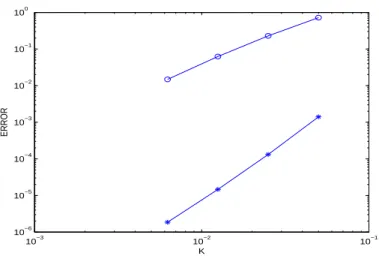
Figure 1: Local error (*) and global error (o) with vanishing boundary conditions

For the sake of brevity, we will restrict the proof of∥∆−₀1ρn∥H2_(Ω)=O(k3) to the case of the assumptions of Theorem 3. Notice that, in such a case, if we allow to use unbounded operators ∆0, by using (13), we can writewn(k) in (26)

as

wn(k) =u(tn) +i

k

2f(|u(tn)| 2_)u(t

n) +ik∆u(tn)

−(I+ik∆0φ1(ik∆0))(

k2

8 f(|u(tn)| 2₎2_u(t

n) +

k3

48f(|u(tn)| 2₎3_u(t

n) +· · ·)

−k2

2 (I+ik∆0φ2(ik∆0))∆(f(|u(tn)| 2_)u(t

n))

−k2(1

2I+ik∆0φ3(ik∆0))∆ 2_u(t

n).

By inserting this in

∆−₀1ρn+1= ∆−01

[

eik2f(|wn(k)| 2₎

wn(k)−u(tn+1)

] ,

and making the corresponding asymptotic expansions on k, it can be checked that the coefficient ofk2 _{vanishes and that ofk}3 _{is bounded inH}2_{(Ω) because} of the hypotheses of regularity. Moreover, because of the same hypothesis,the expression is continously differentiable intn and therefore one more power ofk

can be obtained for the difference∥∆−₀1(ρn₋j+1−ρn₋j)∥H2_(Ω).

7. Numerical experiments

k 0.1 5×10−2 _2.5×10−2 _1.25×10−2

Local order 3.42 3.17 2.97

Global order 1.65 1.87 2.07

Table 1: Orders for the local and global error with vanishing boundary conditions

10−4 10−3 10−2

10−7 10−6 10−5 10−4 10−3 10−2 10−1 100 101

K

ERROR

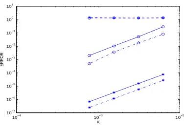
Figure 2: Local error (*) and global error (o) with non-vanishing boundary conditions, avoiding order reduction without conserving symmetry (cont. line), avoiding order reduction conserving symmetry (dash-dotted line) and not avoiding order reduction (discont. line)

k 6.25×10−3 3.125×10−3 1.5625×10−3 7.8125×10−4

Local order 2.26 2.26 2.27

Global order 2.47 2.31 2.40

(1) in Ω = (a, b) withf(x) = 8xand data u0 andg such that the solution is

u(x, t) =eitsech(x)1 + 3 4sech(x)

2_(e8it₋₁₎

1−3₄sech(x)4_sin(4t)2 .

Notice that this solution is very regular and therefore all hypotheses (i)-(v) in Theorems 3 and 7 are satisfied, as well as (29) in Theorems 4 and 8 and (36)-(37) in Theorem 9.

For the space discretization of the Laplacian we will consider the second-order symmetric difference scheme, for which

Ah,0= 1

h2tridiag(1,−2,1), Chg(t) = 1

h2[ga(t),0,· · ·,0, gb(t)]

T_,

wherega(t) andgb(t) are the Dirichlet boundary conditions at the interval

end-points. As Ah,0 is symmetric and its eigenvalues are real, (H1) follows with

M = 1 because the spectral radius of eitAh,0 _{is 1. Moreover, it is well-known} that (5) is satisfied withZ =H4(a, b). Even more, (H2a) is satisfied because if

u∈H4(a, b), ∆−₀1u∈H6(a, b)⊂H4(a, b).

When considering (a, b) = (−50,50), the boundary conditions can be consid-ered as homogeneous and therefore, in such a case, no order reduction is shown when integrating (1) directly through (7) with Strang method. Figure 1, which shows the local and global error against the stepsizekwhen integrating till time

T = 1, corroborates that forh= 1/64. (This value ofhmakes the error in space negligible compared to that in time.) Notice that, in this case, procedure (22) is in fact the same as (7). In fact, Table 1 shows the estimated values of the orders which come from consecutive values of the error and order near 3 can be observed for the local error and near 2 for the global one. Notice that, in this case, the additional values for the boundary ofwn(s) which would be required to

obtain order 3 according to Remark 1, would vanish and therefore this explains that order 3 is observed for the local error.

However, when (a, b) = (0,1), the boundary conditions are not homogeneous any more. Then, applying Strang method directly to (8) as described in the preliminaries gives rise to very bad results which do not even diminish when the considered values of the time stepsizes decrease. That can be observed in Figure 2, whereh= 1/400 has been used for the space discretization. However, when applying the technique (22) which is justified in this paper, order even a bit more than 2 is observed for the local and global errors, as Figure 2 and Table 2 shows. This corroborates Theorems 4 and 9. Moreover, if (22) is applied with

ˆ

Wn

h calculated through (35), the symmetry of the method is conserved and no

order reduction is either shown, as it can be observed in the same figure and in Table 3. Theorem 8 and again Theorem 9 are then corroborated and the numerical results show that the approximation is more accurate.

k 6.25×10−3 _3.125×10−3 _1.5625×10−3 _7.8125×10−4

Local order 2.28 2.27 2.26

Global order 2.17 2.29 2.88

Table 3: Orders for the local and global error with non-vanishing b. c. using procedure (22) with ˆWn

h substituted by (35) and therefore conserving symmetry for Strang method,

h= 2.5×10−3_.

2. In the same way as in that paper, Crank-Nicolson has been used for the integration of (10) and the classical fourth-orderRunge-Kuttamethod for (11). As for the methodswhich are suggested in this paper, we have calculated the terms of the form eikAh,0_U

h by using the fast sine discrete transform, taking

into account that the eigenvalues and eigenvectors of Ah,0 are well-known in this case and that an argument similar to a fast Poisson solver can be applied. It is clear from Figure 3 that the method in [13] also leads to global order around 2. However, the symmetric methodwhich issuggested in this paper manages to get the same error with less computational time. In more dimensions, the comparison would be morefavourablefor the generalizations of Strang method which are suggested here since the calculation ofzin (10)-(11) would not be so direct and would imply an additional cost.

10−2 10−1 100

10−4 10−3 10−2 10−1 100

cpu

error

Acknowledgements

This research has been supported by Ministerio de Ciencia e Innovaci´on project MTM2015-66837-P.

References

[1] I. Alonso–Mallo, Runge-Kutta methods without order reduction for linear initial boundary value problems, Numerische Mathematik 91 (2002), 577–603.

[2] I. Alonso–Mallo and B. Cano, Spectral/Rosenbrock discretizations without order reduction for linear parabolic problems, Appl. Num. Math. 47 (2002), 247-268.

[3] I. Alonso–Mallo, B. Cano and J. C. Jorge, Spectral-Fractional Step Runge-Kutta Discretizations for Initial Boundary Value Problems with Time-Dependent Boundary Conditions, Math. Comput. 73 (2004), 1801-1825.

[4] I. Alonso–Mallo, B. Cano and N. Reguera, Analysis of order reduction when integrating linear initial boundary value problems with Lawson methods, submitted for publication.

[5] I. Alonso–Mallo, B. Cano and N. Reguera, Avoiding order reduction when integrating linear initial boundary value problems with Lawson methods, submitted for publication.

[6] I. Alonso–Mallo, B. Cano and N. Reguera, Avoiding order reduction when integrating linear initial boundary value problems with exponen-tial splitting methods, submitted for publication.

[7] C. Audiard, On the non-homogeneous boundary value problem for Schr¨odinger equation, Discret. Cont. Dyn. Sys. 33 (9) (2013), 3861-3884.

[8] C. Bu, K. Tsutaya and C. Zhang , Nonlinear Schr¨odinger Equation with Inhomogeneous Dirichlet Boundary Data, J. Math. Phys. 46 (2005), 083504.

[9] M. P. Calvo and C. Palencia, Avoiding the order reduction of Runge-Kutta methods for linear initial boundary value problems, Math. Com-put. 71 (1997), 1529–1543.

[10] B. Cano and A. Gonz´alez-Pach´on, Projected explicit Lawson methods for the integration of Schr¨odinger equation, Numerical Methods for Partial Differential Equations 31 (1) (2015), 78–104.

[12] L. C. Evans, Partial Differential Equations, American Mathematical Society, Providence, Rhode Island, 1998.

[13] L. Einkemmer and A. Ostermann, Overcoming order reduction in diffusion-reaction splitting. Part 1: Dirichlet boundary conditions, SIAM J. Scientific Computing 37 (3) (2015), A1577–A1592.

[14] E. Faou, A. Ostermann and K. Schratz, Analysis of exponential split-ting methods for inhomogeneous parabolic equations, IMA J. Numer. Anal. 35 (1) (2015), 161–178.

[15] E. Hairer, S. P. Norsett and G. Wanner, Solving Ordinary Differen-tial Equations I. Nonstiff problems, Springer-Verlag Berlin Heidelberg, 1993.

[16] M. Hochbruck and A. Ostermann, Exponential integrators, Acta Nu-merica (2010) 209-286.

[17] A. Pazy, Semigroups of Linear Operators and Applications to Partial Differential Equations,