Effect of the operating temperature on hydrodynamics and membrane parameters in pressure retarded osmosis

Effect of the operating temperature on hydrodynamic and membrane

parameters in pressure retarded osmosis process.

Khaled Touati

, Fernando Tadeo

, Thomas Schiestel

, Christopher Hänel

a

Department of Systems Engineering and Automatic Control, University of Valladolid, 47011 Valladolid,

Spain.Tel: +34 983423162; Fax: +34 983423161. * fernando@autom.uva.es

b

Fraunhofer Institute for Interfacial Engineering and Biotechnology IGB, Nobelstrasse 12, 70569 Stuttgart, Germany. Tel: +49 711970-4401; Fax: +49 711970-4200.

ABSTRACT

The osmotic energy recovered by Pressure Retarded Osmosis (PRO) from flows of different salinities is affected by the temperature, so the effect of the temperature in different hydrodynamic and membrane parameters is studied here. It is shown that raising the operating temperature of the system leads to a modification of the hydrodynamic characteristics of the feed and draw solutions, and an improvement of the intrinsic membrane parameters. Consequently, the energy recovered is higher at high operating temperatures. These results are validated with laboratory results using solutions at different concentrations and temperatures.

Keywords: Pressure Retarded Osmosis, Osmotic Energy, Temperature effects.

1.

Introduction

Harvesting clean energy to satisfy the ever-growing energy demand of human society is of great importance for the sustainable development of human civilization [1]. Water and energy are inextricably linked and mutually dependent, with each one affecting the other’s availability. Pressure retarded osmosis (PRO) is one of the processes that shows the strong link between water and energy [2]. The PRO process uses the osmotic pressure as a driving force to produce power. The first exploitations of osmotic power via PRO processes were carried about 40 years ago [3]. This is achieved by an asymmetric membrane separating two streams with different salinity. Water molecules are spontaneously transported through a semi-permeable membrane, from a low salinity stream (such as river water, brackish or waste water), at ambient pressure, into a pressurized high salinity stream (seawater or brine), with the aid of the osmotic pressure gradient across the membrane [4]. The diluted draw solution, with a greater volume and/or pressure, moves a turbine to produce electricity. In 2009, Statkraft built the world’s first PRO osmotic power plant [5] showing that power densities higher than 5W/m2 are required for a commercially viable PRO process [6].

1 _{Funded by Mineco Project DPI2014-54530-R}

and FEDER funds

The potential for energy extraction from this “salinity potential” resource (for all river effluents combined) amounts to around 2.4/2.6 TW, close to present day global electricity consumptions [7]. In the near future, PRO systems could be considered an effective form of power production from renewable energy sources, alongside other established renewable technologies (e.g., solar and wind) [7]. However, several challenges have already been identified, especially concerning membrane development [8].

2 PRO background

In PRO, feed and draw solutions are separated by a semi-permeable membrane; so water spontaneously permeates through the Membrane from the feed to the draw solution, driven by the osmotic pressure difference across the membrane [4]. The ideal osmotic process can be described by the thermodynamic equations for the water and salt fluxes. The general equations of transport are [13]:

𝐽𝐽𝑤𝑤 = 𝐴𝐴 (∆𝜋𝜋𝑚𝑚 − ∆𝑃𝑃) (1)

𝐽𝐽𝑠𝑠 =𝐵𝐵(𝐶𝐶𝐷𝐷,𝑚𝑚− 𝐶𝐶𝐹𝐹,𝑚𝑚) (2)

where Jw is the water flux, Js is the salt flux, A is the water permeability coefficient of the membrane, B is the salt permeability coefficient of the membrane, CD,mand CF,m are the solute concentrations at the interface of the active and support layers, respectively, ∆𝜋𝜋_𝑚𝑚 is the difference between osmotic pressures at the surface of the active layer, and ∆P is the hydraulic pressure applied on the draw water side. A schematic of the salt concentration profile across a membrane operating in PRO mode (active layer facing the draw solution) is shown in Figure 1.

With the use of an asymmetric membrane, internal concentration polarization (ICP) occurs in the porous layer of the membrane, which reduces the osmotic driving force across the active layer, and thus the water flux. In PRO, the orientation of the Active dense Layer facing the Draw Solution (AL–DS) is considered to be mechanically more stable, as the external hydraulic pressure is applied on the draw side [11,12]. In this case, concentrative ICP occurs in the porous layer of the membrane.

Due to the ICP within the porous support, reverse salt permeation across the membrane, and the External Concentration Polarization (ECP) in the draw solution, the effective osmotic driving force is lower than the osmotic pressure difference between the bulk draw and feed solutions. Thus, a more realistic water flux expression is:

𝐽𝐽𝑤𝑤 = 𝐴𝐴 (𝜋𝜋𝐷𝐷,𝑚𝑚 – 𝜋𝜋𝐹𝐹,𝑚𝑚− ∆𝑃𝑃) (3) (3)

where πD,m and πF,m are the osmotic pressures at

the surface of the active, and support layers, respectively. Taking into consideration the effect of ICP and ECP on the driving force, and assuming that the osmotic pressure is proportional to the concentration and the temperature (𝜋𝜋=𝛽𝛽𝐶𝐶𝛽𝛽𝛽𝛽), the water flux expression is given by [4]:

𝐽𝐽𝑤𝑤=𝐴𝐴 �𝜋𝜋𝐷𝐷,𝑏𝑏𝑒𝑒𝑒𝑒𝑒𝑒�−

𝐽𝐽𝑤𝑤

𝑘𝑘�−𝜋𝜋𝐹𝐹,𝑏𝑏𝑒𝑒𝑒𝑒𝑒𝑒(𝐽𝐽𝑤𝑤𝐾𝐾)

1+_{𝐽𝐽𝑤𝑤}𝐵𝐵[𝑒𝑒𝑒𝑒𝑒𝑒(𝐽𝐽𝑤𝑤𝐾𝐾)−1] − ∆𝑃𝑃� (4)

where πD,b is the bulk osmotic pressure of the draw solution near the surface of the active layer, πF,b is the bulk osmotic pressure of the feed solution near the surface of the support layer, β is the van’t Hoff coefficient, R is the universal gas constant, and T is the absolute temperature. The mass transfer coefficient k is defined as [7]:

𝑘𝑘=𝑆𝑆ℎ𝐷𝐷_𝑑𝑑

ℎ (5)

where D is the diffusion coefficient of the solute in the draw solution, Sh is the Sherwood number and dh is the hydraulic diameter of the flow channel defined as:

𝑑𝑑ℎ=_𝑃𝑃4𝑆𝑆_𝑤𝑤 (6)

where S is the area of the flow section and Pw is the hydrated perimeter.

The solute resistivity K is defined as [14]:

𝐾𝐾 =𝜏𝜏𝑡𝑡𝑠𝑠_{𝜀𝜀𝐷𝐷}=_𝐷𝐷𝑠𝑠 (7)

where ε, τ , ts and s are, respectively, the porosity, tortuosity, thickness and structure parameter.

The specific salt flux in PRO, defined as the ratio of salt flux to water flux, Js/Jw, is affected by the intrinsic transport properties of the membranes, as follows [15]:

𝐽𝐽𝑠𝑠

𝐽𝐽𝑤𝑤=

𝐵𝐵

𝐴𝐴𝐴𝐴𝐴𝐴𝐴𝐴 �1 +

𝐴𝐴𝐴𝐴𝑃𝑃

𝐽𝐽𝑤𝑤� (8)

where β is the van’t Hoff coefficient, R is the universal gas constant, and T is the absolute temperature.

C

,b

J

C

m

C

m

Feed solution

Draw solution

∆π

x

x

δ

t

C

b

J

Support layer

Fig.1: A schematic representation of the salt concentration profile and water fluxes across a

membrane in PRO at steady state.

3 Effect of the operating temperature on the

feed and draw solution chemistry

3.1 The Osmotic Pressure

The difference in osmotic pressure between bulks is an important factor in PRO: In fact, it is the driving force of the process. The feed solution concentration is in general assumed to have a very low concentration, whereas the draw water solution has a high concentration, so as to achieve an appropriate difference of values between the osmotic pressures. The temperature has a significant impact on the thermodynamic properties of the water. In fact, referring to the van’t Hoff equation (𝜋𝜋=

𝛽𝛽𝐶𝐶𝛽𝛽𝛽𝛽), the osmotic pressure is is directly

proportional to the temperature. It must be pointed out that, for solutions with a very high concentration, the osmotic pressure is not proportional to the concentration; however, the assumption of proportionality between the osmotic pressure and the temperature is still applicable: for example, following the results in [16], the expression of the osmotic pressure at a given temperature T, as a function of the concentration C for a NaCl solution can be approximated by:

𝜋𝜋= 𝛽𝛽𝐴𝐴(3.805𝐶𝐶2+ 42.527𝐶𝐶+ 0.434) (9)

where TR is the normalized temperature:

𝛽𝛽𝐴𝐴= ₂₇₃𝐴𝐴_.15 (10)

For simplicity’s sake, NaCl solutions are now considered: Figure 2 shows the expected effect of the temperature on the osmotic pressure of the draw water for different concentrations.

Fig.2: Osmotic pressure of NaCl solution at different temperatures and concentrations

following Eq.(9).

It can be seen that the osmotic pressure increases when the temperature of the solution increases. However, the effect of the temperature on the osmotic pressure is more significant when the concentration of the water is more important: When the concentration is 0.2 M, the pressure gain is around 1.5 bar when the temperature is raised from 15 to 60°C; whereas the gain is around 7 bars for 1M. Referring to Eq. (1), as the water flux through the membrane is proportional to the difference of osmotic pressures, then, using a high temperature clearly leads to a better driving force to the process. In PRO processes, the driving force is directly related to the draw solution concentration, which explains the enhanced water flux at higher draw solution concentrations. It is clear that much higher power density can be obtained using brines of high osmotic pressures (such as seawater RO brine, MED brine, the Dead Sea water)[25].

3.2 The Diffusion coefficient D

The Diffusion coefficient D is an important parameter in PRO as the mass transfer of feed solution k and solute resistivity K are proportional to D. This coefficient has a strong dependence on the temperature and the concentration of the solution. This diffusion coefficient can be calculated empirically using the Stokes-Einstein relationship [17]:

𝐷𝐷= 𝑘𝑘𝑏𝑏𝐴𝐴

6𝜋𝜋𝜋𝜋𝜋𝜋𝜋𝜋 (11)

where kb is the Boltzmann Constant, µ is the kinematic viscosity of the NaCl solution, T is the temperature of the solution, r is the ion radius and ρ is the density of the solution. The empirical equations have been proposed to estimate the kinematic viscosity as [18]:

𝜋𝜋

𝜋𝜋𝑤𝑤= 1 + 𝑒𝑒𝐶𝐶𝑆𝑆𝑒𝑒𝑒𝑒𝑒𝑒 �

𝐶𝐶𝑠𝑠𝑓𝑓

𝑔𝑔𝐴𝐴𝑅𝑅+𝑖𝑖� (12)

where 𝜇𝜇_𝑤𝑤is the water’s kinematic viscosity at temperature T, where e = 0.12, f = 0.44, g = 3.713, and i = 2.792 are the fitting parameters (values given for NaCl solutions), and CS the molar concentration

The temperature also affects the dynamic viscosity 𝜈𝜈. For example, this dependence was described in [19] for NaCl solutions as follows:

𝜈𝜈(𝛽𝛽) = 2.414 × 10�_{𝑇𝑇−140}247.8−5� ₍₁₃₎

Using Eq. (11)-(13), Fig. 2 shows the effect of temperature on the diffusivity of the water 0

10 20 30 40 50 60 70

10 20 30 40 50 60

O

sm

o

ti

c p

re

ssu

re

(

b

a

r

)

Temperature (°C)

through the membrane. It can be seen that in the range of temperature studied, the value of the diffusion coefficient is almost tripled. At low temperatures (from 15⁰C to 20⁰C), the effect of the solution concentration on the diffusivity is

not significant, as compared to high

temperatures, where it becomes more

considerable. This is due to the fact that the NaCl solution is considered a blending of an attractive interaction between particles when interactions between particles within the solvent took place. When the temperature goes up, the viscosity of the solution decreases and the interaction between the particles is reduced due to thermal agitation. Thus, the diffusion coefficient tends to decrease as concentration increases.

Fig.2: Diffusion coefficient of NaCl solutions at different temperatures and concentrations.

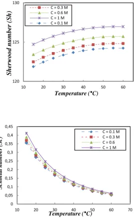
3.3 Reynolds, Schmidt and Sherwood

numbers

The mass transfer coefficient (k) depends on the relevant physical properties of the fluid, the geometry used along with relevant dimensions, and the average velocity of the fluid if we are considering flow in an enclosed conduit, or the approach velocity if the flow is over an object. Dimensional analysis can be used to express this dependence in dimensionless form. The dimensionless version of the mass transfer coefficient is the Sherwood number (Sh). The Sherwood Number depends on the Reynolds number (Re), and the Schmidt number (Sc). The Sherwood number is then defined as [20]:

𝑆𝑆ℎ = 0.04 𝛽𝛽𝑒𝑒0.75_{𝑆𝑆𝑆𝑆}0.33 _{(Turbulent flow) (14)}

𝑆𝑆ℎ= 1.85�𝛽𝛽𝑒𝑒.𝑆𝑆𝑆𝑆𝑑𝑑ℎ

𝐿𝐿� (Laminar flow) (15)

where L is the length of the water channel and dh is the hydraulic diameter of the flow channel. The Reynolds and Schmidt numbers are calculated as follows:

𝛽𝛽𝑒𝑒=𝑉𝑉.𝑑𝑑_𝜋𝜋.𝜋𝜋=𝑉𝑉_𝑣𝑣.𝑑𝑑 (16)

𝑆𝑆𝑆𝑆=_{𝜋𝜋𝐷𝐷}𝑉𝑉 (17)

where V is the velocity of the water, d is the diameter of the pipe, 𝜌𝜌 is the density of the water, 𝑣𝑣 the dynamic viscosity of the fluid, and

𝜇𝜇 is the cinematic viscosity.

As shown in Eqs. (16) and (17), the dimensionless numbers Re and Sc depend on

parameters which also depend on the

temperature, such as the viscosity and the diffusion coefficient. Fig.4 shows that, at high temperatures, the effect of the concentration on Sc is negligible. Contrary to the Sc number, the concentration effect seems to be non-significant at low temperatures. Raising the temperature of the process leads to the modification of the flow regime from laminar to turbulent, because of the strong effect of the temperature on the Re value. In the case of NaCl solutions, the effect of the concentration is not significant. In fact, the variation of the viscosity and density of the water, within the range of concentrations studied, was not so important as to affect the dimensionless parameters Re. For real fluids (seawater, brine wastewater...), the result should be similar, due to the fact that the Reynolds number is not strongly affected by the concentration, as shown in Fig.5-a. However, the matrix complexity of real fluids can affect the viscosity. For seawater and brine, these effects are negligible, because more than 75% of the matrix is NaCl; but for wastewater, the composition of the matrix is generally uncontrollable as it contains organic matter, dissolved polymeric waste, etc…, which strongly affect the viscosity of the flows and their velocities.

2 4 6 8 10

10 20 30 40 50 60

D (

1

0

-9 m 2/s)

Temperature (°C)

C = 0.1 M C = 0.3 M C = 0.6 M C = 1 M

60000 80000 100000 120000 140000 160000 180000

10 20 30 40 50 60

R

eyn

o

ld

s

n

u

m

b

er

(

R

e)

Temperature (°C)

C = 0.1 M C = 0.3 M C = 0.6 M C = 1M

Fig. 5: (a) Reynolds, (b) Schmidt and (c) Sherwood numbers of NaCl solutions at different temperatures, following (14)-(17).

4 Effect of the operating temperature on the

membrane parameters

4.1 The boundary layer thickness δ

It is well known that when a viscous fluid flows along a fixed impermeable wall or past the rigid surface of an immersed body, the velocity at any point on the wall or other fixed surface is zero. The extent to which this condition modifies the general character of the flow depends upon the value of the viscosity. If the body is of a streamlined shape, and if the viscosity is small, the effect appears to be confined within (narrow regions adjacent to the solid surfaces) boundary layers. A boundary layer may be laminar or turbulent. A laminar boundary layer is one where the flow takes place in layers, each layer sliding past the adjacent layers. Laminar boundary layers are found only when the Reynolds numbers are small. A turbulent boundary layer, on the other hand, is marked by mixing across several layers. Thus, there is an exchange of mass, momentum and energy on a much bigger scale as compared to a laminar boundary layer. A turbulent boundary layer forms only at larger Reynolds numbers. Eq.(18) and (19) describe the thickness of the boundary layer for different flow regimes [22]:

𝛿𝛿= 5_{�𝐴𝐴𝑒𝑒}.0×𝑒𝑒

𝑥𝑥 (Turbulent flow) (18)

𝛿𝛿=𝑒𝑒 0.382

(𝐴𝐴𝑒𝑒𝑥𝑥) 1 5

(Laminar flow) (19)

where the distance x is along the membrane (see fig.1) and Rex is the local Reynolds number. It has been shown that, when the thickness of the boundary layer is smaller, the mass transfer is more important [21]. The effect of the temperature on the thickness of the boundary layer was studied. Fig. 6 shows that the effect of the concentration is not really comparable to the effect of the temperature on the boundary layer thickness. The boundary layer has an important dependence on the regime of the flow: as the Reynolds number becomes larger, the viscous effects are not as important at the front of the boundary layer, but become much more important near the end of the boundary layer. Also, the larger the Reynolds number, the thinner the boundary layer becomes. Thus, when the temperature of the water becomes important, the viscosity of the solution is reduced, which leads to an increase in the value of the Reynolds number. In summary, the increase of the operating temperature leads to a thinner boundary layer and a higher mass transfer across it.

Fig.6: The thickness of the boundary for NaCl solutions at different temperatures, following

(18).

4.2 Effect of the temperature on the mass

transfer coefficient k

The process of Mass Transfer across an interface in the bulk of a phase is the result of a chemical potential driving force, which is usually expressed in terms of concentrations of the species. The rate of transfer of a given species per unit area normal to the interface, i.e., the flux, depends on some of the physical properties of the system and on the degree of Turbulence of the phases involved. As the relationship between the flux and these 120

125 130

10 20 30 40 50 60

She

rw

o

o

d

num

b

er

(

Sh)

Temperature (°C)

C = 0.3 M C = 0.6 M C = 1 M C = 0.1 M

0 0,05 0,1 0,15 0,2 0,25 0,3 0,35 0,4 0,45

10 20 30 40 50 60 70

Sc

hm

id

t

num

b

er

(

Sc

)

Temperature (°C)

C = 0.1 M C = 0.3 M C = 0.6 C = 1 M

3 3,5 4 4,5 5

10 20 30 40 50 60

δ

(1

0

-4m)

Temperature (°C)

parameters is not easily developed from fundamentals of mass transfer, coefficients have been defined that lump them all together. These definitions are of the form: Flux = coefficient

×(Concentration difference). [23]

In the PRO case, the mass transfer coefficient (k) characterizes the transport of water from the feed solution to the draw solution through the active layer. The mass transfer coefficient described in Eq. (5) depends on parameters that also depend on the temperature. In this section, the effect of the temperature on the mass transfer coefficient is studied experimentally. Four draw solutions with different concentrations were tested (0.1M, 0.3M, 0.6M and 1M of NaCL), whereas the concentration of the feed water was kept equal to 0.00855M of NaCl. The applied pressure ∆P was half of the osmotic pressure difference between each of the two solutions. Experimental results are shown in figure 7. Similar to the other parameters studied, k is significantly affected by the working temperature. The value of k was quadrupled in the range of temperature studied. However, the effect of the solution concentration is not significant at low temperatures. The experimental result seems to be in correlation with the previous sections. In fact, the mass transfer coefficient depends strongly on the diffusivity and the boundary layer. As shown in figure 2 and 6, high temperatures lead to high diffusivity and low boundary thickness. According to film theory, a high diffusivity with a thin boundary layer enhance the rate of mass transfer [26].

Fig.7: The mass transfer coefficient (k) for NaCl solutions at different temperatures

(experimental results).

4.3 Effect of the temperature on the solute

resistivity K

The solute resistivity (K), described as in Eq. (7), is a parameter used to determine the

influence of the internal concentration

polarization on the water flux. Smaller K value means less ICP, resulting in higher pure water

flux. To determine K experimentally for different operating temperatures, a rearrangement of Eq. (4) was used, as shown below:

𝐾𝐾=_𝐽𝐽1

𝑤𝑤𝑙𝑙𝑙𝑙 �

𝜋𝜋𝐷𝐷,𝑏𝑏𝑒𝑒𝑒𝑒𝑒𝑒�−𝐽𝐽𝑤𝑤� �+_𝑘𝑘 𝐽𝐽𝑤𝑤−𝐵𝐵_𝐴𝐴 +∆𝑃𝑃�1−_{𝐽𝐽𝑤𝑤}𝐵𝐵�

𝜋𝜋𝐹𝐹,𝑏𝑏+𝐵𝐵_𝐴𝐴+∆𝑃𝑃_{𝐽𝐽𝑤𝑤}.𝐵𝐵 � (20)

Experimental results were carried out for two draw solutions (0.6M and 1M of NaCl) and NaCl feed solution (0.00855M). The parameters were calculated using experimental results, performed in the range of temperatures from 15⁰C to 60⁰C. The applied pressure ∆P was always fixed to be half that of the osmotic pressure difference between each of the two solutions.

Fig.8: The solute resistivity (K) for the NaCl solution at different solution temperatures and

concentrations (experimental results).

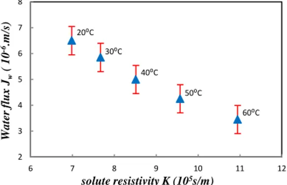
Fig. 8 reveals that, at low temperatures, K is important, and the effect of the concentration of the draw solution on K is clearly considerable. In fact, Eq. (20) shows that K is inversely proportional to the water flux of the membrane, so to reach the best performance, the solute resistivity should be as low as possible. Fig. 9 shows that the solute resistivity tends to reduce the water flux of the process: when K is high, the water flux is significantly smaller. In fact, K depends on the structure parameter s: when s decreases, K decreases too, due to the fact that the membrane becomes thinner when the operating temperature increases. This is due to the simultaneous effect of the temperature and pressure: the increase of the operating temperature makes the membrane polymer softer, so tangential forces caused by the applied pressure reduce s. Thus, to reduce the effect of K on the water flux of the membrane and thus on the energy produced using PRO, it would be better to operate with a high temperature, following the results in Fig. 8 and Fig. 9.

2 4 6 8 10 12 14

10 20 30 40 50 60

k

(

1

0

-4 m

/s)

Temperature (°C)

C = 0.1M C = 0.3M C = 0.6M C = 1M

0,00 0,20 0,40 0,60 0,80 1,00 1,20 1,40 1,60

10 20 30 40 50 60

S

o

lu

te

r

es

is

tiv

ity

K

.

1

0

6 (s

/m

)

Temperature (°C)

Fig.9: Variation of the water flux in PRO with the solute resistivity K (experimental results

with 1M draw and 0.00855M feed NaCl solutions).

4.4 Effect of the temperature on the water

flux (Jw)

The water flux (Jw) at different operating conditions is now studied experimentally: three draw solutions were tested (0.5M, 0.66M and 1M of NaCl) at a range of temperatures varying from 20⁰C to 60⁰C. The feed solution was fresh water (NaCl 0.00855M) and the applied pressure ensured that ∆P was half the osmotic pressure difference between the two solutions. Some experimental results are presented in Fig.10.

As the water flux (Jw) depends on the

concentration of the draw solution, when this concentration is high, the water flux increases due to the high value of the osmotic pressure difference, which is the mean driving force of the system. This can be seen in the experimental results: the water flux increases with the operating temperature for all the tested operating conditions. For example, when the concentration of the draw solution is 1M, the water flux doubled from 20⁰C to 60⁰C, so the energy that can be produced could also be doubled. This result can be attributed to the variation of the transport parameter of the membrane due to the temperature. In fact, this increase of the water flux is due to the improvement of the water permeability of the membrane (A), which depends strongly on the temperature, and the improvement of the mass transport coefficient (k), as shown in section 4.3.

Fig. 10 shows the experimental variation of the salt flux (Js) as a function of the temperature, at different draw solution concentrations. As expected, the salt flux increases when the draw solution concentration is high. It can also be seen that Js increases when the temperature increases. This is a negative effect, as the

reverse solute diffusion can cause a significant reduction in both the PRO water flux and the power density: Draw solutes diffusing through the membrane accumulate in the porous substrate due to the water flux that has the opposite flow direction. This leads to a buildup of draw solute concentration within the porous support layer, contributing to the increase of the ICP at the surface of the support layer, in turn leading to a decrease in the effective osmotic pressure difference and the water flux.

The reverse solute diffusion occurs

simultaneously with the forward water

permeation in the reverse direction. A useful quantity is the specific solute flux (Js/Jw) that describes the amount of draw solutes permeating through the membrane normalized by the volumetric water flux. The study of the ratio (Js/Jw) at different temperatures (see Fig. 11) reveals that, at low temperatures (T< 35⁰C), the increase of the water flux is dominant as compared to the increase of the salt flux. However, when the temperature of the draw is significantly high the plot of (Js/Jw) tends to a horizontal shape which means that the dominance of the water flux is clearly reduced. Thus, the diffusion of salt from the draw solution into the support layer becomes more important which induces a severe internal concentration polarization. This result reveals that working at high temperature still limited by the undesirable effect of the solute diffusion, due to its correlation with ICP and membrane fouling, which increases at high temperatures for a flat sheet membrane.

Fig.10: variation of the water flux Jwand the salt flux Js with the PRO temperature at 2

3 4 5 6 7 8

6 7 8 9 10 11 12

Wa

te

r f

lu

x

Jw

( 1

0

-6.m

/s)

solute resistivity K (105_s/m)

20⁰C

30⁰C

40⁰C

50⁰C

60⁰C

0 1 2 3 4 5 6 7

15 25 35 45 55 65

Wa

te

r f

lu

x

Jw

(1

0

-6 m

/s)

Temperature (⁰ C)

C = 1M C= 0.66 M C = 0.5M

(a)

0 0,5 1 1,5 2 2,5 3 3,5 4

15 25 35 45 55 65

S

a

lt

f

lu

x

J

s

[g

/(s

.m

²)].

1

0

-2

Temperature (⁰ C)

C = 0.5M C =0.66M C = 1M

different draw solution concentrations. (experimental results).

Fig.11: variation of the ratio (Js/Jw) with the PRO temperature at different draw solution

concentrations. (experimental results).

5 CONCLUSION

The effect of the temperature on the Pressure Retarded Osmosis process has been investigated. It was shown experimentally that the temperature affects many parameters of the membrane and the hydrodynamic characteristics of the feed and draw solutions. It has been shown that, in general, working at high temperatures increases the water flux of the process, and consequently the power recovery. The disadvantages of high temperatures are the risk of accumulation of salt at the surface of the membrane support layer, due to the fact that raising the temperature also leads to the increase of the salt reverse flux (Js), and the degradation of the membrane. These can be overcome by the development of specific high-temperature membranes with a high resistance to reverse salt flux.

ACKNOWLEDGEMENTS

This work was co-funded by the seventh

framework program, under grant 288145 (H2OCean), within the ocean of tomorrow joint call 2011.

LIST OF SYMBOLS

A Water permeability coefficient. (m.s-1_.Pa-1₎

B Salt permeability coefficient. (m.s-1₎

CD,m Salt concentration of the membrane surface at the

draw solution side. (g.l-1₎

CF,m Salt concentration on the membrane surface at the side

of the feed side .(g.l-1₎

CD,b Salt concentration of the feed stream.(g.l-1)

CF,b Salt concentration on the membrane surface at the side

of the feed.(g.l-1)

Cs Molar concentration of NaCl solution. (M)

ΔCm Concentration difference on the membrane surface.(g.l -1₎

dh Hydraulic diameter of the flow channel. (m)

D Diffusion coefficient of the solution. (m2_.s-1₎

d Diameter of the pipe.(m)

Jw Water flux that crosses the membrane. (m/s)

Js Salt fluxthat crosses the membrane. (g/m2.s)

k Mass transfer coefficient. (m.s-1₎

K Solute resistivity. (s.m-1) kb Boltzman constant. (-)

Pw The hydrated perimeter. (m)

ΔP Transmembrane Pressure. (Pa)

Δπ Difference of osmotic pressure between the draw water and the feed water. (Pa)

r Ion radius. (m)

R Gas constant. (J.mol·1_K-1₎

Re Reynolds number. (-) Rex local Reynolds number. (-)

s Structure parameter of the support layer. (m) Sc Schmidt number. (-)

Sh Sherwood number. (-) TR The normalized temperature (-)

TD,b Temperature of the draw water bulk. (°C)

TF,b Temperature of the feed water bulk. (°C)

V velocity of the fluid. (m/s)

η Dynamic viscosity of the solution. (Pa.s)

πD,m Osmotic pressure at the surface of the active layer. (Pa)

πF,m Osmotic pressure at the surface of the support layer.

(Pa)

πD,b Osmotic pressure at the draw bulk. (Pa)

πF,b Osmotic pressure at the feed bulk. (Pa)

ts Length of the support layer. (m)

τ Tortuosity of the membrane. (-) ε Porosity of the membrane. (-) β van't Hoff coefficient. (-)

δ Thickness of the boundary layer. (m) ρ Density of the solution. (kg/ m3₎

µw Water kinematic viscosity. (m2/s)

REFERENCES

[1] W. Guo, L. Cao, J. Xia, F.Q. Nie, W. Ma, J. Xue, Y. Song, D. Zhu, Y. Wang, and L. Jiang, Energy Harvesting with Single-Ion-Selective Nanopores: A Concentration-Gradient Driven Nanofluidic Power Source, Adv. Funct. Mater. 20 (2010) 1339–1344.

[2]W. Xu, H. Zhongmai, L. Lei, H. Shusheng, Y. Eileen Hao, K. Scott, Energy generation from osmotic pressure difference between the low and high salinity water by pressure retarded osmosis, J. Technol. Innov. Renew. Energy. 1 (2012) 122-130.

[3] S. Loeb, Production of energy from concentrated brines by pressure retarded osmosis. I. Preliminary technical and economic correlations, J. Membr. Sci. 1 (1976) 49–63. [4] H. Gang, S. Zhang, L. Xue, C. Tai-Shung, High performance thin film composite pressure retarded osmosis (PRO) membranes for renewable salinity gradient energy generation, J. Membr. Sci. 440 (2013) 108–121.

[5] S.E. Skilhagen, J.E. Dugstad, R.J. Aaberg, Osmotic power—Power production based on the osmotic pressure difference between waters with varying salt gradients. Desalination, 220 (2008) 476–482.

0,00 0,20 0,40 0,60 0,80 1,00 1,20

15 25 35 45 55 65

Js /Jw

(g

.m

-1).

1

0

4

Temperature (⁰ C )

[6] B. Simen, Ø. Skråmestø, S. Stein, E. Skilhagen, Osmotic Power From prototype to industry – what will it take? 3rd International Conference on Ocean Energy, Bilbao, October 2010.

[7] A. Achilli, T.Y. Cath, A. E. Childress, Power generation with pressure retarded osmosis: An experimental and theoretical investigation, J. Membr. Sci. 343 (2009) 42–52. [8] Z. Jia, B. Wang, S. Song, Y. Fan, Blue energy: Current technologies for sustainable power generation from water salinity gradient, Renew. Sustainable Energy Rev. 31 (2014) 91– 100.

[9] Q. She, X. Jin, C. Y. Tang, Osmotic power production from salinity gradient resource by pressure retarded osmosis: Effects of operating conditions and reverse solute diffusion, J. Membr. Sci. 401– 402 (2012) 262– 273.

[10] Y. Xu, X. Peng, C.Y. Tang, Q.S. Fu, S. Nie, Effect of draw solution concentration and operating conditions on forward osmosis and pressure retarded osmosis performance in a spiral wound module, J. Membr. Sci. 348 (2010) 298–309.

[11] T.Y. Cath, A.E. Childress, M. Elimelech, Forward osmosis: principles, applications, and recent developments, J. Membr. Sci. 281 (2006) 70–87.

[12] S. Chou, R. Wang, L. Shi, Q. She, C. Tang, A. Gordon Fane, Thin-film composite hollow fiber membranes for pressure retarded osmosis (PRO) process with high power density, J. Membr. Sci. 389 (2012) 25– 33.

[13] K.V. Peinemann, K. Gerstandt, S.E. Skilhagen, T. Thorsen, T. Holt, Membranes for Power Generation by Pressure Retarded Osmosis, in Membranes for Energy Conversion, Volume 2 (eds K.-V. Peinemann and S. Pereira Nunes), Wiley, Weinheim, Germany (2008). [14]C.Y. Tang, Q. She, W.C.L. Lay, R. Wang, A.G. Fane, Coupled effects of internal concentration polarization and fouling on flux behavior of forward osmosis membranes during humic acid filtration,J. Membr. Sci. 354 (2010) 123–133.

[15] Q. She, D. Hou, J. Liu, K. Hai Tan, C.Y. Tang, Effect of feed spacer induced membrane deformation on the performance of pressure retarded osmosis (PRO): Implications for PRO process operation, J. Membr. Sci. 445 (2013) 170–182.

[16] S. Phuntsho, S. Hong, M. Elimelech, H.K. Shon, Osmotic equilibrium in the forward osmosis process: Modelling, experiments and implications for process performance, J. Membr. Sci. 453 (2014) 240–252.

[17] J.S. Collura, D.E. Harrison, C.J. Richards, T.K. Kole, M.R. Fisch, The Effects of Concentration, Pressure, and Temperature on the Diffusion Coefficient and Correlation Length of SDS Micelles, J. Phys. Chem. B 105 (2001) 4846–4852.

[18] S. J. You, X. H. Wang, M. Zhong, Y.-J.Zhong, C. Yu, N. Q. Ren, Temperature as a factor affecting transmembrane water flux in forward osmosis: Steady-state modeling and experimental validation, Chem. Eng. J. 198–199 (2012) 52–60.

[19] A. Tarik, Engineering Fluid Mechanics, first edition (2012), pp. 17–18.

[20] G. Carbonell,Mass transfer coefficients in

coiled tubes, Biotechnology and

Bioengineering, 17 (1975) 1383–1385.

[21] M.C.Y. Wong, K. Martinez, G.Z. Ramon, E.M.V. Hoek, Impacts of operating conditions and solution chemistry on osmotic membrane structure and performance, Desalination 287 (2012) 340–349.

[22] P.J. Pritchard, Introduction to Fluid Mechanics, Wiley, 2011.

[23] A.H.P. Skelland, (1974) Diffusional Mass Transfer. John Wiley.

[24] K. Touati, A. de la Calle, F. Tadeo, L. Roca, T. Schiestel, D.C. Alarcón-Padilla, Energy recovery using salinity differences in a multi-effect distillation system, Desal. Wat. Treat. (2014, in press) 1–8.

[25] L.G. Palacin, F. Tadeo, C. Prada, H. Elfil, K. Touati, Evaluation of the recovery of osmotic energy in desalination plants by using pressure retarded osmosis, Desal. Water Treat. 51 (2013) 360–365.