Reduced Computational Cost in the Calculation of
Worst Case Response Time for Real Time Systems
José M. Urriza, Lucas Schorb
Facultad de Ingeniería- Departamento de Informática Universidad Nacional de la Patagonia San Juan Bosco
Puerto Madryn, Argentina e-mail: [email protected]
Javier D. Orozco, Ricardo Cayssials
Departamento de Ingeniería Eléctrica y Computadoras Universidad Nacional del Sur - CONICET
Bahía Blanca, Argentina e-mail: [email protected]
Abstract— Modern Real Time Operating Systems require reducing computational costs even though the microprocessors become more powerful each day. It is usual that Real Time Operating Systems for embedded systems have advance features to administrate the resources of the applications that they support. In order to guarantee either the schedulability of the system or the schedulability of a new task in a dynamic Real Time System, it is necessary to know the Worst Case Response Time of the Real Time tasks during runtime. In this paper a reduced computational cost algorithm is proposed to determine the Worst Case Response Time of Real Time tasks.
Keywords- Schedulability; Response Time Analysis; RM; DM
I. INTRODUCTION
Nowadays there exist several Real Time Operating
Systems (RTOS). Among the best known we can name:
ChibiOS/RT, eCos, FreeRTOS, Fusion RTOS, Nucleus RTOS, OSE, OSEK, QNX, RT-11, RTEMS, RTLinux, Talon DSP RTOS, Transaction Processing Facility, and VxWorks, among others.
The most popular, probably, is that developed by Wind River Systems, VxWorks, for its use in: The Spirit and Opportunity Mars Exploration Rovers, The Mars Reconnaissance Orbiter, The Deep Impact space probe, Stardust (spacecraft), The Boeing 787 airliner, The Boeing 747-8 airliner, The BMW iDrive system, Linksys WRT54Gxx wireless routers, to name some of the devices that have the RTOS of this company. Its main features are, its simplicity and that can guarantee that a hard Real Time System (RTS) can be scheduled by the discipline of fixed priorities, Rate Monotonic (RM).
In VxWorks, in order to ensure the schedulability of all tasks, the RTOS limits the maximum utilization factor admissible for the system, through an upper bound presented in 1973 by Liu & Layland in [1]. Its main advantage is to have a negligible ComputationalCost (CC), in exchange for providing pessimistic results which imply an over-dimensioning of the system.
The election of this method by Wind River Systems ([2]) is probably due to their low CC, or perhaps because the new
methods, which have been developed, have higher CC in comparison with the one of Liu & Layland. While this statement is true, it also shows a fertile field to explore the discipline in order to obtain the analytical techniques with
low CC, even when they are higher than the bound
established by Liu & Layland. This increase is rewarded by a better utilization of resources or by a better treatment of systems with more complex requirements
Below is a brief introduction to the RTS.
A. Introduction to the Real Time Systems
In the classical definition (Stankovic’s [3]): RTS are those in which results must not be only correct from an arithmetic-logical point of view but also produced before a certain instant, called deadline.
Depending on the deadlines of the tasks, the RTS can be classified into three types. The first one does not allow any task to lose its deadline, so they’re called hard or critical. The second allows to miss some deadlines, so they are called soft. Finally, the further dissemination of RTS has required typify those that allow only a certain amount of loss under a specified statistical criterion. These are called firm.
In the hard RTS, to lose the deadline of a task can have severe consequences for the system integrity and, probably, for the environment, in the case that the system strongly interacts with it: avionics, robotics, etc. In order to guarantee the accomplishment of the tasks before their deadline it is necessary to make an analysis of the schedulability of the system. If the test is successful, it is said that the system is schedulable and ensures the accomplishment of all its temporal constraints.
In [1], the schedulability of mono-resource and multitasking systems is considered. A priority discipline establishes a linear order on the set of tasks, allowing the scheduler to define at each instant of activation, which task will use the shared resource.
To formalize the analysis of schedulability, it is necessary to model the set of tasks based on their temporal requirements and their interdependencies.
after a certain time requests execution. The task is said to be independent if it doesn’t need the result of the execution of some other task for its own execution.
Finally, it is said that the task is appropriable when the scheduler can suspend its execution and withdraw it from the resource at any time.
Generally, the parameters of each task, under this framework, are: its execution time, which is noted as Ci, its
period; noted Ti, and its deadline Di. So a set of n tasks S(n)
is specified by S(n)={(C1, T1, D1), (C2, T2, D2),..., (Cn, Tn,
Dn)}.
In [1] it was proved that the worst generation scheme, for a mono-resource system, is one in which all the tasks request to be executed in the same instant and it is called the critical instant. It was showed also that if this state is schedulable, the RTS is schedulable for any other state, under the priority discipline used.
The utilization factor (U) of a set of hard tasks S(n) determines the level of utilization of the resource.
In [1], the schedulability of the RTS is guaranteed by calculating an upper bound, whose CC is of the order of the number of tasks, because it is needed to calculate the U. If the U is lower than or equal to the level above, it ensures the schedulability of the RTS.
Numerous schedulability tests have been developed since 1973 with the same technique ([4, 5, 6, 7, 8, 9].). In 1982, Leung ([10]), defined Deadline Monotonic (DM), but a schedulability test wasn’t defined. In 1991 Audsley ([11]) presented a solution for this problem. In 1986, Joseph and Pandya ([12]) presented an iterative method of Fixed Point (FP) to evaluate a necessary and sufficient condition to validate the feasibility of an RTS, using a RM scheduler. Several works have been published with equivalent solutions in [13, 14, 15, 16]. In 1998, Sjödin ([17]) incorporated an improvement to Joseph’s test. Which is to begin the iteration of the task i+1 at the moment where the method of Joseph found the worst case response time (WCRT) of task i plus the execution time of task i +1 ( 0
1 m
i i i
t+ =t +C).
In 2004, Bini ([18]) proposed a new method called
Hyperplanes Exact Test (HET) to determine the
schedulability of an RTS.
The paper is organized as follows: Section 2 describes the FP iterative methods used to determine the schedulability of an RTS. Furthermore it proves theorems to improve the search of the mentioned FPs. In section 3, an example is presented. In section 4, the CC of the proposed method with the CC of the algorithms presented in Real Time literature are compared. The analysis results are presented in Section 5. In Section 6, the conclusion and further works are presented
II. FIXED POINT ITERATIVE METHODS
Since 1986, most of the schedulability tests developed for the disciplines of fixed priorities RM or DM, are based on
applying a FP method for ensuring the necessary and
sufficient condition that guarantee the feasibility of the system.
By definition, a FP of a function f is a number t, such that t= f t( ). As in this case the FP equation is a function of time. A tpoint and a tinstant, are equivalent expressions.
The method of FP for an RTS, was first developed by Joseph and Pandya ([12]). In this method, it is proved that there isn’t an analytical construction to resolve such problems and it is only possible to calculate it by iterative computations.
Joseph’s method is initialized in the critical instant where all the tasks are simultaneously invoked. As shown in [12], the result is the WCRT of task i, of a subset of tasks
S(i). Below is the same equation with only a change in nomenclature and the addition of a superscript (q) to indicate in which iteration is:
1 1
1
q i q
i j j j
t
t C C
T
− +
=
⎡ ⎤
= + ⎢ ⎥
⎢ ⎥
∑
(1)The solution, if it exists, is only valid when there is a FP
( q1 q
i i
t + =t ) and if the response time to attend the task i, is lower than or equal to its deadline ( q
i i
t ≤D ).
A. Iterative algorithm
Following is the analysis of Joseph’s iterative method, in order to propose from this analysis, an algorithm to obtain the FP with a lower CC.
Suppose a schedulable RTS,S(n) = {(C1, T1, D1), (C2, T2,
D2),..., (Cn, Tn, Dn)}.
When applying the method of [12] to a task i, with
1
i ∈ < ≤i n, m +1 iterations will occur before reaching a FP with m≥0. Below is a generic trace:
Iteration 0:
0 0 0
1
1 2 1
1 2 1
... i i
i
t t t
C C C C t
T T T− −
⎡ ⎤
⎡ ⎤ +⎡ ⎤ + + + =
⎢ ⎥
⎢ ⎥ ⎢ ⎥
⎢ ⎥ ⎢ ⎥ ⎢ ⎥
Iteration 1:
1 1 1
2
1 2 1
1 2 1
... i i
i
t t t
C C C C t
T T T− −
⎡ ⎤
⎡ ⎤ +⎡ ⎤ + + + =
⎢ ⎥
⎢ ⎥ ⎢ ⎥
⎢ ⎥ ⎢ ⎥ ⎢ ⎥
...
Iteration m-1:
1 1 1
1 2 1
1 2 1
...
m m m
m i i i
t t t
C C C C t
T T T
− − −
− −
⎡ ⎤
⎡ ⎤ +⎡ ⎤ + + + =
⎢ ⎥
⎢ ⎥ ⎢ ⎥
Iteration m:
1
1 2 1
1 2 1
...
m m m
m m i i
i
t t t
C C C C t t
T T T
+ −
−
⎡ ⎤
⎡ ⎤ +⎡ ⎤ + + + = =
⎢ ⎥
⎢ ⎥ ⎢ ⎥
⎢ ⎥ ⎢ ⎥ ⎢ ⎥
Since it is a FP equation and all FP is an attractor, if the subsystem S(i) is schedulable, the equation has at least one FP. The iterative process will evolve to the first FP in the ascendant chain, as shown by Kleene’s Theorem and in [19]. Reached the FP in tm, the result of the iteration m-1(tm)
must be equal to the result of the iteration m (tm+1). What
follows is an analysis of the equation ⎡⎢t T Cj⎤⎥ j and the
conditions under which the FP method ends.
The calculation of ⎡⎢t Tj⎤⎥ determines the number of
instances of task j in the interval [0, t ). Then, ⎡⎢t T Cj⎤⎥ j
indicates the accumulated runtime of all instances of task j to instant t, also known as the workload of task j (W tj( )).
Therefore, under the assumption that the scheduler can’t leave the resource idle while there are instances of tasks to execute, the equation will find an FP when the sum of all execution times of all instances of the tasks is equal to the time required to execute them.
To obtain the time where there will be an invocation of the task j, after time t, should be multiplied ⎡⎢t Tj⎤⎥ by the
period of the task (Tj ). When ⎢⎣t T T/ j⎥⎦ jis calculated, the time
when the nearest instance is reached, corresponding to time t is obtained. Therefore, in the interval [⎣⎢t T Tj⎦⎥ j,⎡⎢t T Tj⎤⎥ j), the
calculation of the equation ⎡⎢t T Cj⎤⎥ j with any t within this
interval has the same value.
Due to the previous analysis, it is desirable to indicate the workload of task j at instant t of the iteration q as:
with 0 and 1 1
q q
j j
j
t
A C q m j i
T ⎡ ⎤
=⎢ ⎥ ≤ ≤ ≤ ≤ −
⎢ ⎥
When it is replaced in the development of the trace, starting from a seed value t0, we have:
Iteration 0:
1 0 0 0
1 2 ... i 1 i
t =A +A + +A− +C
Iteration 1:
2 1 1 1
1 2 ... i 1 i
t =A +A + +A− +C
...
Iteration m-1:
1 1 1
1 2 ... 1
m m m m i i
t =A − +A − + +A−− +C
Iteration m:
1
1 2 ... 1
m m m m i i
t + =A +A + +A− +C
Either if the RTS is not feasible to be scheduled by RM or DM, the algorithm does not converge or it converges in a time later than the deadline of the analyzed task. Therefore, the inspection interval of the algorithm is reduced from the critical instant to the deadline ((0,Di]).
B. Improvements for the Iterative Algorithm
The previous section provides that, if Equation (1) has a solution (FP) the iterations m-1 and m will have the pairs
1, with 1 1
m m j j
A − A ≤ ≤ −j i equal. Therefore, if this condition is not met, the algorithm will perform at least one more iteration to find the FP.
In Joseph’s algorithm, in each iteration of Equation (1), the initialization of the variable t, is done with the value obtained in the previous iteration. That is why if q
j
A is
different to q1
j
A − , the calculation of the 1,...., 1
q q j i
A+ A− is not
affected. Basically, in each iteration, the variable t is initialized with the sum of:
1
1 1
1
i
q q q q
j j j
t t A A
−
− +
=
= +
∑
− (2)The Equation (2) is determined by taking the Equation (1) in two successive iterations, with q≥0:
1 1
1 1
1 1
0 and 0
i i
q q
q q
i j i j
j j
t C A t C A
− −
− +
= =
− −
∑
= − −∑
=Consequently, the method requires successive iterations so the changes occurring in the current iteration affect the calculation of the following 1,...., 1
q q j i
A+ A− .
Iteration 1:
0 0 0
1 2 1
1
1 1
1
.... i i
A A A C
A C
T
−
+ + + +
⎡ ⎤
= ⎢⎢ ⎥⎥
0 0 0
1 2 1
1
2 2
2
.... i i
A A A C
A C
T
−
+ + + +
⎡ ⎤
= ⎢⎢ ⎥⎥
...
0 0 0
1 2 1
1
1 1
1
.... i i
i i
i
A A A C
A C
T
−
− −
−
+ + + +
⎡ ⎤
Iteration 2:
1 1 1
1 2 1
2
1 1
1
.... i i
A A A C
A C T − + + + + ⎡ ⎤ = ⎢⎢ ⎥⎥
1 1 1
1 2 1
2
2 2
2
.... i i
A A A C
A C T − + + + + ⎡ ⎤ = ⎢⎢ ⎥⎥ ...
1 1 1
1 2 1
2
1 1
1
.... i i
i i
i
A A A C
A C T − − − − + + + + ⎡ ⎤ = ⎢⎢ ⎥⎥ ...
Iteration p-1:
2 2 2
1 2 1
1
1 1
1
....
p p p i i p A A A C
A C T − − − − − ⎡ + + + + ⎤ = ⎢ ⎥ ⎢ ⎥
2 2 2
1 2 1
1
2 2
2
...
p p p i i p A A A C
A C T − − − − − = ⎢⎡ + + + + ⎤ ⎥ ⎢ ⎥ ...
2 2 2
1 2 1
1
1 1
1
....
p p p i i p i i i
A A A C
A C T − − − − − − − − ⎡ + + + + ⎤ = ⎢ ⎥ ⎢ ⎥
Iteration p:
1 1 1
1 2 1
1 1
1
....
p p p i i p A A A C
A C T − − − − ⎡ + + + + ⎤ = ⎢ ⎥ ⎢ ⎥
1 1 1
1 2 1
2 2
2
....
p p p i i p A A A C
A C T − − − − ⎡ + + + + ⎤ = ⎢ ⎥ ⎢ ⎥ ...
1 1 1
1 2 1
1 1
1
....
p p p i i p i i i
A A A C
A C T − − − − − − − ⎡ + + + + ⎤ = ⎢ ⎥ ⎢ ⎥
Illustrated in the equations showing the trace (Iteration 1), the calculation of 1
1
A is not used in the calculation of 1 2
A
and so on. All the 1
j
A of the first iteration are used to
calculate all the 2
j
A of the second iteration. The question
arises: Is it possible to use the 1,...,
q q j
A A with j< −i 1 already
calculated to estimate the following 1,..., 1
q q j i
A+ A− belonging to the same iteration? The answer is yes.
The improvement that is proposed to Joseph’s algorithm to reduce its CC, is to initialize the variable t, in the same iteration, with a new value. Each time that q q1
j j
A >A− , it is known that in the iteration q the FP that satisfies the Equation (1) will not be found, and, consequently the algorithm will not stop. Therefore, as shown in Theorem 1, when it meets that q q1
j j
A >A− , it is valid to increase t with the
difference q q1
j j
A −A− . The new value ( tq+ ) is used to calculate the following 1
q j
A+ , and so on. Therefore, t is initialized with:
1
q q q q
j j
t+= +t A −A− (3)
This way, it is possible to calculate the following
1,..., 1
q q j i
A+ A− of the iteration q, with the calculation of the first
1,...,
q q j
A A of the same iteration and not of the previous one. This improvement of the algorithm allows that p iterations will only be needed to reach the same FP with p≤m.
Below is a trace of how it develops after iteration 0, in which the algorithm is initialized by taking a seed for the variable t0 , and calculating consequently 0 0
1,..., i1
A A− , and
storing it in an array of dimension n-1 . To highlight the previously established is used.
Iteration 1:
0 0 0
1 2 1
1
1 1
1
.... i i
A A A C
A C T − + + + + ⎡ ⎤ = ⎢⎢ ⎥⎥
1 0 0
1 2 1
1
2 2
2
.... i i
A A A C
A C T − ⎡ + + + + ⎤ = ⎢ ⎥ ⎢ ⎥ ⎢ ⎥ ...
1 1 0
1 2 1
1
1 1
1
.... i i
i i
i
A A A C
Iteration 2:
1 1 1
1 2 1
2
1 1
1
.... i i
A A A C
A C T − + + + + ⎡ ⎤ = ⎢⎢ ⎥⎥
2 1 1
1 2 1
2
2 2
2
.... i i
A A A C
A C T − ⎡ + + + + ⎤ = ⎢ ⎥ ⎢ ⎥ ⎢ ⎥ ...
2 2 1
1 2 1
2
1 1
1
.... i i
i i
i
A A A C
A C T − − − − ⎡ + + + + ⎤ = ⎢ ⎥ ⎢ ⎥ ⎢ ⎥ ...
Iteration p-1:
2 2 2
1 2 1
1
1 1
1
....
p p p i i p A A A C
A C T − − − − − = ⎢⎡ + + + + ⎤ ⎥ ⎢ ⎥
1 2 2
1 2 1
1
2 2
2
...
p p p i i p A A A C
A C T − − − − − =⎡⎢ + + + + ⎤⎥ ⎢ ⎥ ⎢ ⎥ ...
1 1 2
1 2 1
1
1 1
1
....
p p p i i p i i i
A A A C
A C T − − − − − − − − ⎡ + + + + ⎤ ⎢ ⎥ = ⎢ ⎥ ⎢ ⎥
Iteration p:
1 1 1
1 2 1
1 1
1
....
p p p i i p A A A C
A C T − − − − ⎡ + + + + ⎤ = ⎢ ⎥ ⎢ ⎥ 1 1
1 2 1
2 2
2
....
p p p i i p A A A C
A C T − − − ⎡ + + + + ⎤ ⎢ ⎥ = ⎢ ⎥ ⎢ ⎥ ... 1
1 2 1
1 1
1
....
p p p i i p i i i
A A A C
A C T − − − − − ⎡ + + + + ⎤ ⎢ ⎥ = ⎢ ⎥ ⎢ ⎥
Note in the trace that in iteration 1, the 1 1 1 1, 2,..., i 2
A A A− are
used to calculate 1 1
i
A− .
Theorem 1:
Given a feasible RTS, the proposed method converges to the same FP as Joseph’s method.
Proof:
Let tPF the time when the first FP happens. Then
for a seed t0 , with 0
PF
t ≤ t , Joseph’s method
converges to the lowest FP (Kleene’s theorem
proved in [12]). A new algorithm that does not meet the same FP, can only be possible if the basin of attraction of tPF is jumped. For this to happen
with a monotonic increasing and deterministic function, it must be obtained with the algorithm a
PF
t> t and end in the basin of attraction of other
FP, or not converge. But the increment in the
variable t, within the iteration, is obtained with the
same function
(
q)
j j
t T C
⎡ ⎤
⎢ ⎥ and is used by Joseph’s
method in the following iteration (Equation (2)). Since the new algorithm proposes that with each
1
q q j j
A >A− will be incremented tq with q q1
j j
A −A− ,
the calculation of q j
A is done with tq. So if every
time that a pair q q1
j j
A >A− is found, tq is increased
making q q q q1
j j
t += +t A −A− , and it is bounded by an upper and lower limit of Joseph’s function, calculated in tq and in tq+.
1 1
1 1
q q
i i
q
i j i j
j j
j j
t t
C C t C C
T T + − − + = = ⎡ ⎤ ⎡ ⎤ + ⎢ ⎥ ≤ ≤ + ⎢ ⎥ ⎢ ⎥ ⎢ ⎥
∑
∑
With q q q q1
j j
t+= +t A −A− and1≤ ≤ −j i 1
As this calculation is bounded by the function of Joseph, that can be iterated from point tq+ and the minor FP be found, it’s not possible that the presented algorithm obtains a time that skips the minor FP. □
Theorem 2:
Proof:
In an iteration q with tq different to a FP, there
exists at least one 1
with 1 1
q q j j
A− ≠A ≤ ≤ −j i . This increment produces, in the algorithm of Joseph, an increment in tq that will be computed in the
following iteration (Equation (2)). May be that, if for the value of tq+1 there is an q q1
y y
A ≠A+ with
1
j< ≤ −y i , two iterations to approach the FP in
1
2 ( q q ) ( 1 )
q q q q
y y j j
t + = +t A −A− + A+ −A will be computed. In the proposed algorithm this occurs in the same iteration, due that the calculation of q
y
A is done
with q q q q1
j j
t += +t A −A − , then resulting
1
1 q q 1
q q q q q q q y y j j y y
t ++=t++A −A− = +t A −A− +A −A− . □
C. The Proposed Algorithm
The proposed algorithm requires two arrays for storing the WCRT and q
j
A . These arrays are called WCRTi and Aj.
Function Test
1
t=C
For i = 2to n
:
r i
t =t t= +t C : Flag = 1 DoUntil( tr=t or t>Di)
: 0 r
t =t w=
For j=1to i-1
j j
A= ⎢⎡t T⎤⎥C
If Flag = 0and A≠Aj then
j
t= + −t A A
If t > Dithen Test = False: Exit ‘Not schedulable
End If
j
A =A:w= +w A
Next
t = Max (t, w): Flag = 0 Loop
WCRTi = tr: Flag = 1
Next
Test =True ‘The system is schedulable EndFunction
III. EXTENSION:BLOKING TIME AND RELEASE JITTERS
This section extends the proposed analysis to the case of shared resources and release jitters.
The analysis presented in [Audsley, 1993 #181] can be applied to the calculation of schedulability in the RTS presented in this paper.
The worst case of blocking by lower priority tasks, that a task i can receive, when using the ceiling priority protocol [Sha, 1990 #214], is defined as Bi.
The release jitter time (Ji) is the worst-case time that task
i can spend waiting to be released after its arrival. In the analysis made in previous sections the release jitter time does not present any problem to be calculated since it is a constant.
The equation 1 is as follows:
1 1
1
q i
i q
i i j j j
t J
t B C C
T
− +
=
⎡ + ⎤
= + + ⎢ ⎥
⎢ ⎥
∑
IV. AN EXAMPLE
Given an RTS with the following parameters: S(4) = {(2,4,4), (1,5,5), (2,6,6), (1,12,12) }.
With the method of Sjödin for task 4, the iteration starts in t = 5.
4 1 1
0 1
4 4
5 5 5
5 1 .2 .1 .1 7
4 5 6
t = → = +t ⎡ ⎤⎢ ⎥ +⎡ ⎤⎢ ⎥ +⎡ ⎤⎢ ⎥ = ⎢ ⎥ ⎢ ⎥ ⎢ ⎥
4 2 2
1 2
4 4
7 7 7
7 1 .2 .1 .1 9
4 5 6
t = → = +t ⎡ ⎤⎢ ⎥ +⎡ ⎤⎢ ⎥ +⎡ ⎤⎢ ⎥ = ⎢ ⎥ ⎢ ⎥ ⎢ ⎥
6 2 2
2 3
4 4
9 9 9
9 1 .2 .1 .1 11
4 5 6
t = → = +t ⎡ ⎤⎢ ⎥ +⎡ ⎤⎢ ⎥ +⎡ ⎤⎢ ⎥ = ⎢ ⎥ ⎢ ⎥ ⎢ ⎥
6 3 2
3 4
4 4
11 11 11
11 1 .2 .1 .1 12
4 5 6
t = → = +t ⎡ ⎤⎢ ⎥ +⎡ ⎤⎢ ⎥ +⎡ ⎤⎢ ⎥ =
⎢ ⎥ ⎢ ⎥ ⎢ ⎥
6 3 2
5 5
4 4
12 12 12
12 1 .2 .1 .1 12
4 5 6
t = → = +t ⎡ ⎤⎢ ⎥ +⎡ ⎤⎢ ⎥ +⎡ ⎤⎢ ⎥ =
⎢ ⎥ ⎢ ⎥ ⎢ ⎥
With the proposed method the iterations are:
4 1 1
0 1
4 4
5 5 5
5 1 .2 .1 .1 7
4 5 6
t = → = +t ⎡ ⎤⎢ ⎥ +⎡ ⎤⎢ ⎥ +⎡ ⎤⎢ ⎥ = ⎢ ⎥ ⎢ ⎥ ⎢ ⎥
4 2 2
1 2
4 4
7 7 8
7 1 .2 .1 .1 9
4 5 6
t = → = +t ⎡ ⎤⎢ ⎥ +⎡ ⎤⎢ ⎥ +⎡ ⎤⎢ ⎥ = ⎢ ⎥ ⎢ ⎥ ⎢ ⎥
6 3 2
2 3
4 4
9 11 12
9 1 .2 .1 .1 12
4 5 6
t = → = +t ⎡ ⎤⎢ ⎥ +⎡ ⎤⎢ ⎥ +⎡ ⎤⎢ ⎥ =
⎢ ⎥ ⎢ ⎥ ⎢ ⎥
6 3 2
3 4
4 4
12 12 12
12 1 .2 .1 .1 12
4 5 6
t = → = +t ⎡ ⎤⎢ ⎥ +⎡ ⎤⎢ ⎥ +⎡ ⎤⎢ ⎥ =
⎢ ⎥ ⎢ ⎥ ⎢ ⎥
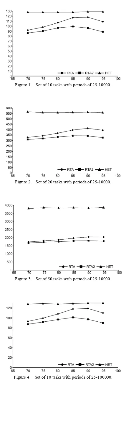
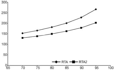
V. EXPERIMENTAL RESULTS
The simulations consist in counting how many units q j
A
are required to calculate for the proposed algorithm (RTA2)
and for the method of Sjödin ([17]) denominated RTA
(Response Time Analysis), and for the method of Bini ([18]) denominated HET.
The q j
A is the invariant for the proposed method and for the method of Sjödin ([17]).
For the method of Bini ([18]) an invariant of one or two calculations, of the type q
j
A , can be counted.
In [18], the way to measure the computational cost is by counting how many loops are performed to determine if the system is schedulable.
Unfortunately, the introduced CC is not evaluated by the invariant of method, and does not take into account that a recursive method introduces a space charge in the management of recursions.
Therefore, counting each time that this type of account happens, the results of the three methods are comparable.
Subsequently the total average of how many units q j
A for U is calculated.
Experiments were conducted with two groups of tasks. In the first set, the election of the period and the execution time of each task were performed in a random way with a uniform distribution. The selected groups used periods between 25-10000 and 25-25-100000 ticks.
The periods of tasks in the second group were divided into subgroups by order of magnitude. Subgroups were constructed with 25-100, 101-1000, 1001-10000 ticks and another with 25-100, 101-1000, 1001-10000 and 10001-100000.
For example, for 10 tasks with periods between 25- 10000, the first 3 task periods were randomly chosen between 25-100, with an exponential distribution centered at 50. The following 3 tasks used periods in the order of 101-1000 centered on 500, and the remaining 4 with periods in the order of 1001-10000 centered on 5000. A similar form was used in [9, 21, 22].
The utilization factors in these groups are comprehended between the 70% and the 95%, in jumps of a 5% with a tolerance of the ±0.5%. Furthermore, for each utilization factor, at least 10000 systems for each U were evaluated. The U lower than 70%, were not considered, because under the
[image:7.595.317.531.89.808.2]≈70% (ln 2*100) the boundary of Liu & Layland ([1]) guarantees the schedulability of the RTS when the number of tasks is infinite. The number of tasks of the groups was 10, 20 and 50.
[image:7.595.325.526.100.432.2]Figure 1. Set of 10 tasks with periods of 25-10000.
[image:7.595.322.526.429.729.2]Figure 2. Set of 20 tasks with periods of 25-10000.
Figure 3. Set of 50 tasks with periods of 25-10000.
Figure 5. Set of 20 tasks with periods of 25-100000.
[image:8.595.323.526.118.251.2]Figure 6. Set of 50 tasks with periods of 25-100000.
[image:8.595.324.525.281.407.2]Figure 7. Set at U = 90% for periods of 25-10000 and 25-100000.
Figure 8. Set of 10 tasks with periods of 25-10000 (subgroups).
Figure 9. Set of 20 tasks with periods of 25-10000 (subgroups).
Figure 10. Set of 50 tasks with periods of 25-10000 (subgroups).
Figure 11. Set of 10 tasks with periods of 25-100000 (subgroups).
[image:8.595.326.522.439.560.2] [image:8.595.50.289.447.561.2] [image:8.595.71.269.596.721.2] [image:8.595.325.526.600.723.2]Figure 13. Set of 50 tasks with periods of 25-100000 (subgroups).
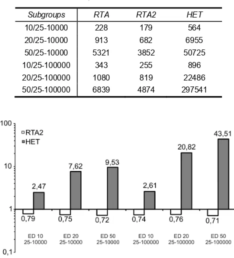
TABLE I. U=90%, PERIODS OF 25-10000 AND 25-100000
Subgroups RTA RTA2 HET
10/25-10000 228 179 564
20/25-10000 913 682 6955
50/25-10000 5321 3852 50725
10/25-100000 343 255 896
20/25-100000 1080 819 22486
50/25-100000 6839 4874 297541
Figure 14. Set at U = 90% for period of 25-10000 and 25-100000.
VI. ANALYSIS RESULTS
The presented method and Bini’s method, when compared with the methods presented by Sjödin (Fig. 7) at U = 90%, it is possible to obtain average reductions between the 11% to the 18% of the CC, depending on the type of the system for a uniform distribution.
For the subgroups simulated with an exponential distribution, the method presented achieved significant improvements that hovered between the 21% to the 29% less CC than the method Sjödin for a U at 90% (Fig. 14). Bini's method for this type of system presented a significant increase in CC and is dependent of the period, although practically constant for the different utilization factors simulated. This is because this method uses a calculation method of hyperplanes.
When there are differences of 2, 3 or 4 orders of magnitude between the periods of the tasks, the method should evaluate each hyperplane in which there is a task with a small period but in conjunction with a task with a period of several orders of magnitude larger, which generates a very large search tree to the method. Unfortunately, this increases exponentially the CC. For this reason, the curves of the method of Bini weren’t shown in the previous figures, but the results, are presented in Table I.
The improvement in the CC of our method is considered important just if we reason that the cost of obtaining it is made just by a single array with dimension n-1. However, the refinement in the algorithm can be used in other kind of methods as the presented in [23] for the calculation of the Slack Stealing, or in methods for Testing the schedulability.
VII. CONCLUSION AND FURTHER WORKS
In this paper is presented a reduced computational cost method to determine the schedulability of a real time system. The method proposed was compared with the most important ones proposed in the real time literature. The results show a reduction in the average computational cost, of between the 11% and 18% for a uniform distribution and a reduction between the 21% and 29% for an exponential distribution in subgroups of different order of magnitude. In further works, the possibility of applying this algorithm to other types of methods will be investigated. New tests with this improvement will be developed.
REFERENCES
[1] C. L. Liu and J. W. Layland, "Scheduling Algorithms for Multiprogramming in a Hard Real-Time Environment," Journal of the ACM, vol. 20, pp. 46-61, 1973.
[2] M. Barabanov, "Best Practices on Wind River Real-Time Core Application Development," Wind River Systems2008.
[3] J. A. Stankovic, "Misconceptions About Real-Time Computing: A Serius Problem for Next-Generations Systems," IEEE Computer, vol. Octubre, pp. 10-19, 1988.
[4] A. K. Mok and D. Chen, "A Multiframe Model For Real-Time Tasks," IEEE Trans. Software Eng., vol. 23, pp. 635-645, 1997. [5] A. Burchard, J. Liebeherr, Y. Oh, and S. H. Son, "New Strategies for
Assigning Real-Time Tasks to Multiprocessor Systems," IEEE Trans. on Computers, vol. 44, pp. 1429-1442, 1995.
[6] C. C. Han, "A Better Polynomial-Time Schedulability Test for Real-Time Multiframe Tasks," in IEEE 19th Real-Time Systems Symposium, 1998, pp. 104-113.
[7] C.-C. Han and H.-y. Tyan, "A Better Polynomial-Time Schedulability Test for Real-Time Fixed-Priority Scheduling Algorithms," in IEEE 18th Real-Time Systems Symp., 1997.
[8] T.-W. Kuo, Y.-H. Liu, and K.-J. Lin, "Efficient Online Schedulability Tests fo Real-Time Systems," IEEE Transactions on Software Engineering, vol. 29, pp. 734-751, August 2003.
[image:9.595.70.270.97.226.2] [image:9.595.52.286.265.523.2]Symposium, IEEE, Ed. Barcelona, Spain: IEEE Computer Society, 2008, pp. 407-418.
[10] J. Y. T. Leung and J. Whitehead, "On the Complexity of Fixed-Priority Scheduling of Periodic, Real Time Tasks," Perf. Eval. (Netherlands), vol. 2, pp. 237-250, 1982.
[11] N. C. Audsley, A. Burns, M. F. Richarson, and A. J. Wellings, "Hard Real-Time Scheduling: The Deadline Monotonic Approach," in
Proceedings 8th IEEE Workshop on Real-Time Operating Systems and Software, Atlanta, GA, USA 1991.
[12] M. Joseph and P. Pandya, "Finding Response Times in Real-Time System," The Computer Journal (British Computer Society), vol. 29, pp. 390-395, 1986.
[13] J. P. Lehoczky, L. Sha, and Y. Ding, "The Rate Monotonic Scheduling Algorithm: Exact Characterization And Average Case Behavior," in IEEE Real-Time Systems Symposium, 1989, pp. 166-171.
[14] J. Santos, M. L. Gastaminza, J. D. Orozco, D. Picardi, and O. Alimenti, "Priorities and Protocols in Hard Real-Time LANs,"
Computer Communications, vol. 14, pp. 507-514, 1991.
[15] J. Santos and J. D. Orozco, "Rate Monotonic Scheduling in Hard Real-Time Systems," Information Processing Letters, vol. 48, pp. 39-45, 1993.
[16] N. C. Audsley, A. Burns, M. F. Richardson, K. Tindell, and A. J. Wellings, "Applying New Scheduling Theory to Static Priority
Preemptive Scheduling," Software Engineering Journal, vol. 8, pp. 284-292, 1993.
[17] M. Sjödin and H. Hansson, "Improved Response-Time Analysis Calculations," in IEEE 19th Real-Time Systems Symp., 1998, pp. 399-409.
[18] E. Bini and C. B. Giorgio, "Schedulability Analysis of Periodic Fixed Priority Systems," IEEE Trans. on Computers, vol. 53, pp. 1462-1473, November 2004.
[19] Z. Manna, S. Ness, and J. Vuillemin, "Inductive Methods for Proving Properties of Programs," Communications of the ACM, vol. 16, pp. 491-502, August 1973.
[20] L. Sha, R. Rajkumar, and J. P. Lehoczky, "Priority Inheritance Protocols: An Approach to Real-Time Synchronization," IEEE TRANSACTIONS ON COMPUTERS, vol. 39, pp. 1175-1185, 1990. [21] R. I. Davis, "Approximate Slack Stealing Algorithms for Fixed
Priority Pre-Emptive Systems," Real-Time Systems Research Group, University of York, York, England, Internal Report1994.
[22] R. I. Davis, K. W. Tindell, and A. Burns, "Scheduling Slack Time in Fixed-Priority Preemptive Systems," Proceedings of the Real Time System Symposium, pp. 222-231, 1993.
[23] J. M. Urriza, J. D. Orozco, and R. Cayssials, "Fast Slack Stealing
methods for Embedded Real Time Systems," in 26th IEEE
International Real-Time Systems Symposium (RTSS 2005) - Work In Progress Session, Miami, EEUU, 2005, pp. 12-16.