Volume 2012, Article ID 651039,18pages doi:10.1155/2012/651039
Research Article
Optimized Carrier Tracking Loop Design for Real-Time
High-Dynamics GNSS Receivers
Pedro A. Roncagliolo, Javier G. Garc´ıa, and Carlos H. Muravchik
LEICI, Facultad Ingenier´ıa, UNLP, B1900TAG La Plata, Argentina
Correspondence should be addressed to Pedro A. Roncagliolo,agustinr@ing.unlp.edu.ar
Received 27 December 2011; Accepted 21 March 2012 Academic Editor: Carles Fern´andez-Prades
Copyright © 2012 Pedro A. Roncagliolo et al. This is an open access article distributed under the Creative Commons Attribution License, which permits unrestricted use, distribution, and reproduction in any medium, provided the original work is properly cited.
Carrier phase estimation in real-time Global Navigation Satellite System (GNSS) receivers is usually performed by tracking loops due to their very low computational complexity. We show that a careful design of these loops allows them to operate properly in high-dynamics environments, that is, accelerations up to 40 g or more. Their phase and frequency discriminators and loop filter are derived considering the digital nature of the loop inputs. Based on these ideas, we propose a new loop structure named Unambiguous Frequency-Aided Phase-Locked Loop (UFA-PLL). In terms of tracking capacity and noise resistance UFA-PLL has the same advantages of frequently used coupled-loop schemes, but it is simpler to design and to implement. Moreover, it can keep phase lock in situations where other loops cannot. The loop design is completed selecting the correlation time and loop bandwidth that minimize the pull-out probability, without relying on typical rules of thumb. Optimal and efficient ways to smooth the phase estimates are also presented. Hence, high-quality phase measurements—usually exploited in offline and quasistatic applications— become practical for real-time and high-dynamics receivers. Experiments with fixed-point implementations of the proposed loops and actual radio signals are also shown.
1. Introduction
A fundamental task of every Global Navigation Satellite System receiver is to synchronize with the visible satellite signals. Since Direct Sequence Spread Spectrum (DS-SS) signals are utilized, code and carrier synchronization is required, but a correlation stage is necessary to despread the signals before the synchronization algorithms can be applied. In real-time receivers the required economy of operations usually precludes the use of complex estimation schemes and tracking loops are preferred. Due to the correlation process these loops are necessarily discrete. The typical trade-offin tracking loop design is bandwidth versus dynamic performance: output noise increases with a larger loop bandwidth, while dynamic tracking error decreases with it [1]. Thus, the loop design becomes particularly challenging when the receivers are subject to high dynamics. To overcome this limitation other receiver structures have been proposed in [1], claiming tracking capability up to 150 g of acceleration, in contrast with the 5 g regularly assigned to tracking loops. However, the required computational burden
is large since several simultaneous correlations and Fast Fourier Transform (FFT) computations are needed. In this paper we show a careful design of the digital loops that can expand their tracking ability to acceleration steps up to 40 g or even more, keeping a low computational load and reasonable tracking threshold values at the same time.
PLL are not based on optimal digital loop solutions, with each loop designed separately, leaving the analysis of their interactions and possible modifications to the simulation stage [2,5,6]. Moreover, schemes adopted to discriminate phase or frequency errors are often justified because of their similarity with well-known analog solutions rather than with an optimality versus implementation complexity criterion. We will show that digital implementations of optimal discriminators are not necessarily more complex and allow designing the FLL-assisted PLL in a coupled way.
Nevertheless, the FLL-assisted PLL leads to a more complex design and a computationally more expensive implementation than a single PLL. Moreover, when coupled-loops lose phase lock for a moment, they present cycle slips introducing a phase ambiguity. We will show how to use the same frequency information as that of an FLL to build a nonambiguous phase detector, the Unambiguous Frequency-Aided (UFA) phase discriminator. A PLL with this new phase discriminator, that is, a UFA-PLL, keeps the desirable properties of an FLL without demanding an extra loop and avoiding cycle slips. Other nonambiguous phase discriminators are known for analog PLLs, that is, with analog loop filter, such as the sequential discriminators built with flip-flops presented in [7,8] or the nonsequential discriminator of [9]. While their goals are quite similar to ours, they increase the PLL implementation complexity, demanding some digital circuitry and a digital-to-analog converter to get the analog phase error. On the contrary, the UFA phase discriminator is easily implemented and naturally suited for a software-based PLL, leading to a less complex implementation than a FLL-assisted PLL. Section2
introduces the UFA-PLL structure for GNSS tracking loops. The optimum loop filter structure for analog PLLs was introduced in [10], solving the mentioned bandwidth trade-off by minimizing a quadratic functional. A widespread technique for designing digital loops is discretizing an analog loop with a sample rate 1/T at least ten times faster than loop bandwidth BN [5, 11, 12]. As BNT increases above
the rule-of-thumb value of 0.1, the resulting loop deviates from optimal and may become unstable [5], especially when accounting for the delays of a digital implementation. This limit imposed to the loop bandwidth is not fundamental and an attempt to avoid it has been presented in [13]. They introduced a digital loop design based on pole placement that allows somewhat largerBNTvalues. However, the pole
location is assigned with standard second-order analog-system rules. Our approach is to consider a completely digital loop model and pose the bandwidth trade-offdirectly in the digital domain, building upon the early and often overlooked work of [14] for hybrid loops. We include two delays in the loop to consider the effect of the correlation stage, similar to the inclusion of an accumulator before the loop error discriminator for signals without spreading codes [15]. Our method [16] allows the design of stable loops with
BNT > 0.1, a particularly useful feature for high-dynamics
receivers. Specifically, we will focus on dynamics modeled as acceleration steps, that is, unbounded jerk, as in the case of launching vehicles when the engine turns on or off. In Section3we first derive the optimal loop filter for arbitrary
phase inputs and then for the case of acceleration steps that produce quadratic ramps of input phase or a linear ramp of the input frequency. Simulations comparing the different loop structures are also shown.
Optimization gives the structure for the loop filter, leaving the choice of T and BN unsolved. Usually, these
parameters are selected based on some rule of thumb [2,5], and the ultimate loop performance, as measured by the pull-out probability and/or tracking threshold, is obtained later by simulation. An optimal choice of these fundamental parameters demands an analysis of the nonlinear aspects of the tracking loop with noise. This is quite difficult, although some results are known for analog loops with relatively simple loop filters, by solving a Fokker-Planck equation [17]. They can be extended to digital loops when an analog approximation is valid [18]. Our approach is to get a reasonable approximation for the pull-out probability and its relationship to the loop parameters. This new approach introduced in [19] allows us considering dynamics modeled as acceleration steps and digital loop filters with zero stationary error response to these inputs. Previous analyses are based on stationary loop responses or sinusoidal acceleration profiles [2,5]. For these cases, we derive approx-imate expressions for the probability of starting a nonlinear behavior of the mentioned loops. These expressions quantify the role ofBNandTand let us choose them in order to obtain
lower tracking thresholds for different dynamic scenarios, as presented in Section4.
Our optimized digital carrier tracking loops also allow smoothing of the phase estimates incorporating more mea-surements, at the expense of some delay. In general, an output delay of a few samples should not be a limitation since the navigation task in a GNSS receiver is usually slow compared with the loop sample rate. This update of the phase estimates can significantly reduce the noise variance and the transient responses in high-dynamics environments. This strategy is suitable for real-time receivers because it can be efficiently calculated. Hence, some of the precise positioning techniques would be applicable in real-time and for high-dynamics receivers. Consider, for instance, smoothing of code delay measurements with carrier phase estimates in stand-alone receivers [12, 20], or differential positioning applications [12,21], or even attitude estimation with GNSS signals [22]. In all these cases, an improvement in the phase estimation has a direct impact on the positioning performance. The expressions for optimal smoothing filters are derived in Section5, and their efficient implementation is also discussed there. In addition, we present experimental results obtained with actual RF signals and a fixed point implementation of our loops tracking acceleration steps of up to 40 g. Finally, the conclusions of this work are given in Section6.
2. Digital Loops Models
φi+nφi
^
φi
z−1
z−1
[·]π
p1
p2
p3
ei
1
1−z−1 1−1z−1 1−1z−1
−
+ +
+ +
+ +
+ +
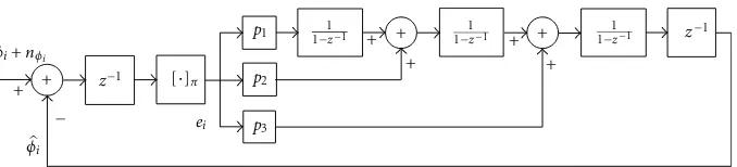
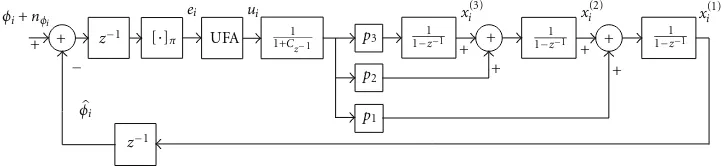
Figure1: Block diagram of classical PLL structure.
carrier power to noise power spectral densityC/N0 and for
theith correlation interval of durationT can be written as [12]
Ci=Di
TC
N0
sinc∆fiR(∆τi)ej(π∆fi+∆θi)+ni, (1)
where ∆τi = τi −τi is the code delay estimation error,
∆fi = fi− fi the frequency estimation error, and ∆θi = θi − θi the phase estimation error, all assumed constant
during the integration time. The sequenceni is a complex
white Gaussian noise process with unit variance,R(·) is the
code correlation function, and sinc(x)=sin(πx)/(πx). It is also assumed that the signal has binary data bitsDi = ±1
and that correlations are computed within a single bit period. This Binary Phase Shift Keying (BPSK) modulation is present in many GNSS signals like the GPS civil signals or in the data components of composite modernized GNSS signals [23].
In tracking conditions (i.e., after the acquisition process has been completed [12]), estimation errors are small and then the functions sinc(·) andR(·) can be approximated by
1. In this case the expression (1) reduces to
Ci=Ii+jQi≈Di
TC
N0
ej∆φi+n
Ii+jnQi, (2)
whereIiandQiare the so-called in-phase and in-quadrature
correlations respectively,nIi = ℜe{ni},nQi = ℑm{ni}, and
we have defined ∆φi = φi −φi, with φi = π fi +θi and
φi = πfi+θi. These sequences allow to model the carrier
tracking loop as a purely digital single-input single-output (SISO) system. When the frequency is changing according to a constant acceleration error of am/s2, we verified—
by numerical integration—that expression (2) is a good approximation ifaT2/λ ≪ 1, whereλis the wavelength of
the signal. For L1 GPSλ =0.19 m and withT = 5 ms, this implies thata ≪ 7600 ≡775 g. In this case, the terms∆fi
and∆φi have to be reinterpreted as the average frequency
error and average phase error during the correlation interval, respectively.
In the following we briefly review the basic concepts of PLL and FLL-assisted PLL from our digital point of view, and later we introduce the UFA-PLL.
2.1. PLL Model. The phase estimation error is typically
obtained using one of several possible discriminators [5],
which give the desired phase modified by different memory-less nonlinearities. The optimal one—maximum likelihood estimator—is given by
ei=tan−1
Q
i
Ii
=∆φi+nφi π, (3)
where the notation [·]π indicates that its argument is kept
within the interval (−π/2,π/2] by adding or subtractingπas
many times as needed. The zero-mean noise termnφi has a
rather complicated probability distribution [24], but in high
C/N0it can be approximated by a Gaussian distribution with
zero mean and varianceσφ2i≈1/(2TC/N0).
A four-quadrant tan−1(
·) is not appropriate if there is
BPSK data modulation because the discriminator becomes sensitive to the data phase changes. On the contrary, for signals without data the range of the discriminator can be doubled with a four-quadrant tan−1(·). We chose this
discriminator because it is not amplitude dependent and the calculation of tan−1(·) can be easily implemented with
a lookup table, since in practice Ii and Qi are frequently
quantized to a few bits.
In order to close the loop in our model, it is of crucial importance to consider the delays present in a real implementation. Failure to account for a delay may turn unstable an optimal loop design. Since ours loops are digital, a single sample delay is expected but in fact there are two. One of them is due to the time spent inIiandQicalculations.
The other delay appears because the estimated values used in the present correlations have to be known before the calculations begin. That is, the value φi is obtained with
the loop filter output of the (i−1)th correlation interval,
which in turn is calculated with the estimation errors ofφi−2.
Then, with these considerations, the model of a PLL using the classical loop filter structure of type 3, that is, with three accumulators, is shown in Figure1.
2.2. FLL-Assisted PLL Model. To add an FLL to our previous
PLL, a frequency discriminator is needed. In a digital loop a frequency error estimate may be obtained as the difference of two successive phase errors, and in fact this is often correct. A problem appears when the discontinuities caused by [·]πmake that the difference to be wrong in±π. However,
our discrete system cannot distinguish frequencies greater than half of the sample rate, that is, phase changes of π
[image:3.600.133.472.70.147.2]φi+nφi
^
φi
z−1
z−1
[·]π
[·]π
p1
p2
p3
ei
1 1−z−1
1
1−z−1 1
1−z−1
−
+ +
+ + +
1−z−1
efi
f1
f2
Figure2: Block diagram of the typical FLL-assisted PLL structure.
frequency errors must lie in the interval (−π/2,π/2] [25].
Thus, the difference of two consecutive outputs of the phase discriminator can be corrected just using the operation [·]π.
Therefore, the frequency discriminator for the FLL can be obtained by
efi=[ei−ei−1]π. (4)
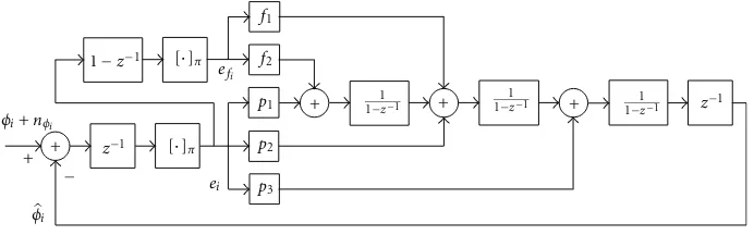
Figure2shows a diagram of the FLL-assisted PLL presented in [2], where the second-order loop filter of the FLL shares the same cascade of accumulators used by the PLL filter.
In the locked conditionei=∆φiandefi =∆φi−∆φi−1
are small enough to justify a linear analysis of the loop. The complete loop is seen as an equivalent PLL with filter coefficients p3, p2+ f2, and p1+ f1, instead of p3, p2, and p1. Thus, the FLL is inserted into the model of the PLL at a
design stage. This eliminates the constrain of using a narrow bandwidth FLL to not significantly perturb the PLL behavior, as in [2,6]. A wide bandwidth FLL allows the loop to have two regions of operation: “phase-locked” as it was described before, and “frequency-locked” when the dynamics unlocks the PLL but the FLL keeps the frequency error within the linear range of its discriminator. In the latter region the loop is governed by the FLL (coefficientsf1andf2) and the phase
error input acts like a zero-mean perturbation [25]. As soon as the dynamics let the loop reduce its frequency error close to zero, the phase lock can be restored.
2.3. The UFA-PLL Model. As we have seen so far, due to the
cyclic nature of phase a memory-less discriminator is unable to distinguish changes of an integer number of cycles—or half cycles if there is BPSK data—, that is, its output is ambiguous. However, it is possible to obtain a frequency error estimate from these ambiguous phase error estimates correcting their difference with the nonlinear operation [·]π.
This is the reason why an FLL can cope with carrier tracking in situations when a single PLL cannot. Assume that there is BPSK data and the PLL phase error is rising and crosses the value π/2. The output of the phase discriminator abruptly changes to a value close to−π/2, reversing the evolution of
the PLL phase. Hence, the phase error will increase since the PLL is now moving in the wrong direction. We should instruct the phase discriminator with information of the phase derivative to keep moving in the right direction, that is, we should feed it with proper frequency information
available at the FLL. Therefore, the idea of the Unambiguous Frequency-Aided (UFA) phase discriminator is to use the same frequency information used by the FLL to get a better phase discriminator. It works correcting the ambiguous values ofeiby adding or subtracting an integer number of πso that the difference of successive values of the corrected phase error, ui, gives the right frequency error. Then, the
equations that define our new phase error estimate, fori∈N,
are
ui=kiπ+ei, kisuch thatIπ(ui−ui−1)=0, (5)
where we defineIπ(x)=x−[x]π, an operation similar to the
function integer part but with steps at the multiples ofπ. A practical formula to computekican be derived noting that Iπ(x+lπ)=Iπ(x) +lπ,l∈Zsince
Iπ(kiπ+ei−ui−1)=kiπ+Iπ(ei−ui−1)=0 (6)
and then kiπ = −Iπ(ei −ui−1). Substituting this in (5),
we can recursively calculate the UFA phase error from the ambiguousei:
ui=ei−Iπ(ei−ui−1) (7)
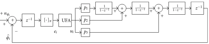
with starting value u0 = e0. Then, the PLL structure in
Figure1transforms into a UFA-PLL just adding a block that implements (7) immediately after the phase discriminator output, as shown in Figure3.
It is interesting to note that the UFA scheme acts like the phase unwrapping algorithm proposed in [18] for correcting cycle slips in the phase estimates of feed-forward synchronizers. In this case, the phase correction does not affect the phase estimation process since it is done once the estimation stage is finished. On the contrary, the UFA phase discriminator modifies the behavior of our feedback estimator, the PLL, changing its nonlinear characteristics. As a result, cycle slips and the rather complex transient responses induced by them are avoided as long as the frequency error is compatible with the loop sample rate.
2.4. Equivalence between UFA-PLL and FLL. We saw that the
[image:4.600.128.474.73.181.2]φ+nφi
^
φi
z−1
z−1 [·]π
p1
p2
p3
ei
1
1−z−1 1−1z−1 1−1z−1
−
+ +
+ +
+ + +
+
ui
UFA
Figure3: Block diagram of the new UFA-PLL structure.
correcting the difference of two consecutive outputs of the phase discriminator just using the operation [·]π. Figure4(a)
shows a block diagram of a digital FLL, with loop filter transfer function F(z). Notice that the two delays and the accumulator that convert the frequency estimation to phase before the feedback are not included inF(z).
An alternative way to obtain the same frequency error discriminator is to use the UFA algorithm previously described. Indeed, the output phase sequence ui is built
in such a way that the difference of consecutive values produces the right frequency error, as seen from (4) and (5). Therefore, the schemes of Figures 4(a) and 4(b) are equivalent. The interesting fact in Figure 4(b)is that most linear blocks are adjacent. Thus, the differentiator cancels with the accumulator without changes in the dynamic loop response, except for the mean value of the phase error, leading to the equivalent UFA-PLL model of Figure 4(c). In fact, this zero-pole cancellation shows why the FLL is insensitive to constant phase errors whereas the equivalent UFA-PLL is not. More importantly, the equivalence reveals that the nonlinear behavior of the UFA-PLL is equal to that of a FLL with the sameF(z), and then their tracking capacity and noise resistance are the same.
3. Optimal Loop Filter Design
We propose to design the digital loop filter minimizing a two-term quadratic functional to handle the bandwidth trade-off
mentioned in the Introduction. The input signal is assumed to have a part related to phase evolutionφiplus additive, zero
mean,and noisenφi. The functional to be optimized is
J=σ2
N+α2ETφi, (8)
where α2 is a weighting factor that controls the
trade-offbetween noise and transient response, that is, the loop bandwidth, σN2 is the noise variance at the loop output,
andET(φi) represents the energy of the tracking error∆φi
transient response. Since the functional uses the energy of the transient response, the optimum filter must produce a zero stationary response for the given input.
Suppose F(z) is the loop-filter transfer function to be found, and consider that the linear model hypothesis holds for a PLL or FLL. The closed loop transfer function including the delays is
T(z)= F(z)z−
2
1 +F(z)z−2 =Y(z)z
−2, (9)
φi+nφi
^
φi
z−1 [·]π [·]π
efi fi+1
F(z)
ei
z−1
1−z−1
− +
+ 1−z
−1
(a) Equivalent scheme with UFA
φi+nφi
^
φi
z−1 [·]
π
efi fi+1
F(z)
ei
z−1
1−z−1
−
+ + 1−z
−1
ui
UFA
(b) FLL scheme
φi+nφi
^
φi
z−1 [·] z−1
π
φi+1
F(z)
ei
− + +
ui
UFA
(c) UFA-PLL equivalent scheme
Figure4: Equivalence between UFA-PLL and FLL.
where Y(z) must be a causal and stable rational transfer function. The minimization of the functional J written in terms of Y(z) is shown in the AppendixA. The optimum transfer function is given by
Y(z)=X(z)z
Ψ(z), (10)
whereΨ(z) andX(z) can be obtained from the spectral fac-torization of (A.6) and from the partial fraction expansion of (A.8), respectively. We repeat them here for completeness,
Ψ(z)Ψz−1=1 +γ2Φ(z)Φz−1, (11)
G(z)=γ
2Φ(z)Φz−1z
Ψ(z−1) =X(z) +W
z−1, (12)
whereΦ(z) is thez-transform of φi. The relation between
[image:5.600.134.473.71.143.2] [image:5.600.309.549.192.446.2]the latter criterion stems from a purely stochastic formula-tion. The connection between both approaches arises when modeling the input phase as white noise passing through a rational transfer function. The Wiener filtering approach offers other possibilities such as keeping the optimality for a wide range of admissible transfer functions via a robust approach as in [27] or considering continuous models for the phase as in [28].
Optimum loop filters for an input phase step, frequency step, and frequency ramp were derived in [16]. In the following, only the last result is presented for the sake of brevity. Analog loop filters optimized for these kind of inputs are the origin of the classical methods of filter design for type one, two, and three loops, respectively. As it will be seen, our purely discrete design for each case has one extra pole, due to the loop delays. This additional pole does not appear when discretizing analog designs, but it has a decisive influence on the stability or the range of achievable productBNT.
3.1. Optimum Filter for a Frequency Ramp. The ramp is
modeled as
Φ(z)= ∆˙ωT
2
(1−z−1)3
, (13)
where ˙∆ω is the rate of frequency change. Denotingν =
˙
∆ω2T4γ2, from (11) it is necessary to solve (z
−1)6−νz3=0.
The six roots of this polynomial are obtained using the fact that three of them are the inverses of the other three. This allows us to express the following equations:
z1,2+z−1,21=2−
1±j√3 2
3
√
ν,
z3+z3−1=2 + 3
√
ν
(14)
that determine the values ofz1,z2, complex conjugates and a
realz3. Using these values and (11), we get
Ψ(z)=
1−z1z−11−z2z−11−z3z−1
(1−z−1)3(z1z2z3)1/2
, (15)
and replacing in (12)
G(z)= −(z1z2z3)
−1/2νz4
z−z1−1
z−z−21
z−z−31
(z−1)3
. (16)
Then, the correspondingX(z) has only three poles inz =1, and the closed-loop transfer function of (10) is
Y(z)= A−Bz−
1+Cz−2
(1−z1z−1)(1−z2z−1)(1−z3z−1), (17)
whereA=(6−3zs+zd),B=(8−3zs+zp), andC=3−zs,
withzs=z1+z2+z3,zp=z1z2z3andzd=z1z2+z1z3+z2z3.
Then, the optimum loop filter with four poles, three of the input and the extra one, is
F(z)= A−Bz−
1+Cz−2
(1−z−1)3(1 +Cz−1)
. (18)
10−6 10−5 10−4 10−3 10−2 10−1 100 101
A
10−1
100
101
BN
T
Figure5: Type 3 loop noise equivalent bandwidth.
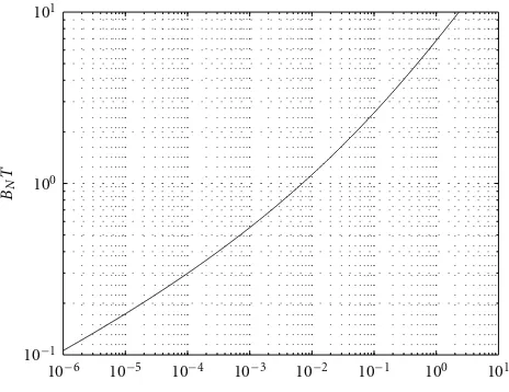
For the purpose of implementation, it is desirable to use a cascade of accumulators. Then, (18) can be rewritten as
F(z)= p3+p2
1−z−1
+p11−z−1
2
(1−z−1)3
1 +p1z−1 , (19)
where p1 = C, p2 = B−2C, and p3 = A−B+C. The
closed loop noise equivalent bandwidth is shown in Figure5. This curve allows choosing the appropriate value ofνfor a
given normalized noise bandwidth. Observe also from this figure that the larger is the step or the parameter ν, the
more emphasis is given to the transient energy, causing the normalized noise bandwidth to increase. The productBNT
levels out to a value of approximately 54.5. This part is not included in the figure since it is of minor importance for most designs of practical interest.
3.2. Design Example: Loops for Launching Vehicles. We
sim-ulate and compare the loop models presented in Section2
taking as an example a GPS carrier tracking loop for launching vehicles [29]. In this case the dynamic input can be modeled as an acceleration step, which becomes a quadratic ramp in terms of phase and a linear one, in terms of frequency. For these inputs the optimal loop filter for a PLL was obtained in Section3.1. The case of an FLL-assisted PLL, taking results from [29], leads to a type 2 FLL and a type 3 PLL.
[image:6.600.313.545.73.252.2]φi+nφi
^
φi
z−1 [ z−1
·]π
[·]π
efi
ei 1+C1z−1
−
+ + +
+
+ +
+
+ 1−z−1
1 (1−z−1)2
f1
f2
p3 1−1z−1
Figure6: Block diagram of the FLL-assisted PLL in Section3.
φi+nφi
^
φi
z−1 [·]π
ei
1 1+Cz−1
+ +
+ +
+
+ +
+
f1
f2
p3 1−1z−1
1
1−z−1 z−
1 1−z−1
UFA
−
Figure7: Block diagram of the UFA-PLL designed in Section3.
in Section4, this rule is not that useful. The resulting filter transfer function for the PLL was
F(z)= A−Bz−
1+Cz−2
(1−z−1)3(1 +Cz−1)
, (20)
whereA = 0.6173,B = 1.105, andC = 0.5. Then, in the structure of Figure1this impliesp1+f1=C=0.5,p2+f2= B−2C =0.105, andp3=A−B+C=0.0123, plus a block
that implements the extra pole inz=−C. The resulting PLL
equivalent noise bandwidth isBN =75.6 Hz.
Since the FLL design does not affect the previous results, it was designed wider than strictly necessary in order to facilitate the posterior implementation. The selected transfer function is
F(z)= D−Ez−
1
(1−z−1)2(1 +Ez−1)
, (21)
whereD=0.6 andE =0.5, resulting in that the extra pole needed for the FLL and the PLL is the same. Then, f1=E=
0.5 and f2 =D−E =0.1. This implisp1 =0 andp2 ≈0.
With these simplifications the complete loop design reduces to the diagram showed in Figure6. This FLL loop can track steps up to 40 g with transient error peaks smaller than 25 Hz, half of the linear range of the frequency discriminator, with an equivalent noise bandwidth ofBN =61.3 Hz.
We will use the previous loop filter as a basis for the comparison of different loop configurations. We consider a PLL and a UFA-PLL with the same loop filter as before, that is p1 = C = 0.5, p2 = 0.105, p3 = 0.0123. This structure
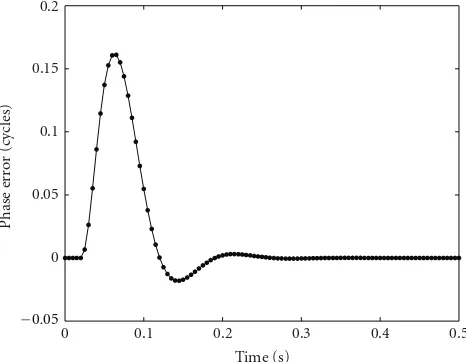
is showed in Figure7. The phase error response for a step of 10 g of acceleration, common to the three loops as expected, is depicted in Figure8. In this case the phase error detected by the discriminators is equal to the actual phase error since its magnitude is always less than a quarter of cycle.
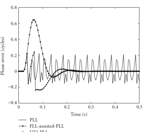
In Figure9the discriminated phase error during a 40 g step in the three loops is illustrated. It can be seen that
0 0.1 0.2 0.3 0.4 0.5
0 0.05 0.1 0.15 0.2
Time (s)
Phase er
ro
r (cy
cles)
−0.05
Figure8: Phase error during a 10 g step.
the PLL cannot track this step, whereas the others can. The response of the UFA-PLL is a scaled version of the response for 10 g, showing the effect of linearization of the discriminator characteristic achieved by the UFA algorithm. In the case of the FLL-assisted PLL the loop lost phase lock for a moment, but could still track the dynamics because the FLL remained locked. This nonlinear behavior could correspond to a cycle slip. To verify this analysis the actual phase error for each configuration is shown in Figure 10. Clearly, there is one cycle slip in the tracked phase of the FLL-assisted PLL, whereas the UFA-PLL is able to track this step of acceleration without any cycle slip.
[image:7.600.128.476.76.152.2] [image:7.600.127.476.205.274.2] [image:7.600.312.545.326.507.2]0 0.1 0.2 0.3 0.4 0.5 0
0.2 0.4 0.6 0.8
Time (s)
Phase er
ro
r (cy
cles)
PLL
FLL-assisted-PLL UFA PLL
−0.4 −0.2
Figure9: Discriminated phase error during a 40 g step.
0 0.1 0.2 0.3 0.4 0.5
0 0.2 0.4 0.6 0.8 1
Time (s)
Phase er
ro
r (cy
cles)
PLL (cycles/100) FLL-assisted-PLL UFA PLL
−0.2
Figure10: Actual phase error during a 40 g step.
as the phase of the PLL does, and the loops will lose their lock. This can be caused by excessively high dynamics or noise power or a combination of both. Notice that the noise power considered in this case is twice the input phase noise power due to the differencing. In fact, we can use the UFA algorithm applied to the frequency discrimination to further extend the dynamics resistance of the loops. However, it will be of little practical importance due to the noise power increase caused by a new differentiation. The frequency error of both loops during a 40 g step is shown in Figure 11. The peak error is 25 Hz—half the limit—and thus, using the same rule of thumb that we used for the phase error of the PLL, it can be argued that 40 g is the level of acceleration steps that can be tracked with a reasonable safety margin for noise effects. In Section4we will give a totally different approach for the consideration of the noise in the UFA-PLL.
0 0.1 0.2 0.3 0.4 0.5
0 10 20 30
Time (s)
F
requency er
ro
r (Hz)
FLL-assisted-PLL UFA PLL
−10
−20
Figure11: Frequency error during a 40 g step.
Another shared feature of the FLL-assisted PLL and the UFA-PLL is the resistance to false locks. For the sake of brevity this analysis is not included here but it can be seen in [16].
4. Pull-Out Probability Analysis
In this section we will compute an approximation to the pull-out probability for a loop in a given operating condition. Since the pull-out is necessarily a consequence of nonlinear behavior, a simple way to bound the pull-out probability is with the probability of entering nonlinear behavior, that is, the limits of the tan−1(
·) range. We are interested in tracking
acceleration steps. Then, it is clear that for a given noise level the instants when the loop is closer to these boundaries approximately correspond to the peaks of the loop transient response. Therefore, we focus on calculating the probability of entering nonlinear behavior at the instant of the transient response peak, given that the loop behavior has been linear up to that time.
4.1. PLL Analysis. The PLL enters nonlinear behavior when
the phase error becomes larger thanπ/2. This is equivalent to a sign reversal of the in-phase component, with respect to the sign of the data bit. Then, the probability of nonlinear behavior at the transient peaki=pis [19]
PP=P
∆φp+nφp
>π
2
=Pcosφp−φp
+n′ Ip<0
,
(22)
wheren′
Ip =DpnI p/
TC/N0has varianceσ2 =1/(2TC/N0).
Assuming that the PLL has had a linear behavior up to the analyzed instant,φp, can be thought of as a deterministic
value plus output noisenφp. Subtracting this deterministic
[image:8.600.55.287.61.274.2] [image:8.600.313.543.72.284.2] [image:8.600.55.287.307.534.2]0 0.025 0.05 0.075 0.1 0.125 0.15 0.175 0.2
0 0.5 1 1.5 2 2.5 3 3.5 4
10−5 10−4 10−3 10−2 10−1
Kp
(cy
cles/g/(10 ms)
2)
A
BN
T
(—)
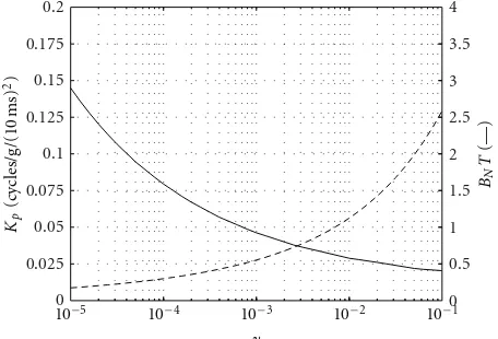
Figure12: Noise Bandwidth and Peak Error Response for type 3
PLL.
response to an acceleration step, which is shown in Figure12
as a function of ν for an integration time of 10 ms. Note
that with acceleration we refer to the Doppler rate the loop has to track, scaled in units of g=9.8 m/s2instead of Hz/s
to keep an easy physical interpretation. This peak value is proportional to the square of the integration time because an acceleration step is a parabolic ramp of phase. The values of the normalized closed-loop equivalent noise bandwidth are also plotted in Figure12for completeness.
The noisenφpdepends on the filtered past input noise—
from instants p−2, p−3, and so on—and is statistically
independent ofn′Ip. Then, we can writeφp−φp=KpaT
2+ nφp, whereais the acceleration amplitude in g’s. In (22), we obtain
PP=P
cosKpaT2+nφp
+n′Ip<0
. (23)
To further simplify (23), we use a “low noise” approximation cos(nφp)≈1 and sin(nφp)≈nφpand obtain
PP≈P
cosKpaT2
−sin
KpaT2
nφp+n′
Ip<0
. (24)
Using central limit theorem arguments, it is reasonable to approximate the distribution ofnφpas a zero mean Gaussian with variance approximated by 2BNTσφ2i ≈ BN/(C/N0),
using the highC/N0variance expression for the input noise.
In this case, both random terms in (24) become a single Gaussian random variable with zero mean and variance (1 + 2BNTsin2(KsaT2))σ2. Therefore,
PP≈Q
⎛ ⎜ ⎝
2TC/N0cos
2K
paT2
1 + 2BNTsin2
KpaT2
⎞ ⎟
⎠, (25)
whereQ(x) is the cumulative Gaussian distribution fromx
to∞. Since the functionQ(√x) is monotonically decreasing, we can define a function
fPLL(ν,T,a)=
2Tcos2K
paT2
1 + 2BN(ν)Tsin2
KpaT2
(26)
0 1
2 3 4 5 6 7 8 9
1 2 3 4 5 6 7 8 9 10
×10−3 ×10−3
T (ms)
10−6 10−4 10−2 100
A
Figure13: FunctionfPLL(ν,T) for type 3 PLL and 5 g.
such that the larger isfPLL, the smaller isPPfor a givenC/N0,
and then a low tracking threshold is attained. For example,
fPLL(ν,T,a) for a 5 g acceleration step is plotted in Figure13.
It can clearly be seen that the larger values of fPLLare found
in the region 5 ms< T <7 ms and 10−3 <ν<100, and the
maximum is approximately atν=0.05 andT =6 ms. The
value of fPLLin this region is about 0.009. Larger values of
νare not preferred because they lead to loops that produce
larger phase estimation error and only a slightly lowerPP.
However, it must be emphasized that for values ofν>10−3
the loop bandwidth isBNT >0.5. These values of bandwidth
show that a filter loop design based on discretization of analog solutions, only valid forBNT <0.1, is not appropriate
to design loops with better tolerance to nonlinear behavior. Ifν=0.02, thenBNT =1.5 and, withT =5 ms, leads to an
optimum loop bandwidthBN = 300 Hz, which is too large
from the point of view of output phase error variance. This shows that the main cause of pull-out in PLLs with narrow bandwidths is the transient error response, due to the input phase and the input noise, rather than output noise. In other words, 5 g of acceleration is very demanding for a single PLL and then a large bandwidth is required to track them with small pull-out probability.
4.2. UFA-PLL Analysis. An equivalent description of the
UFA algorithm presented in Section2is to consider it as a modified tan−1(·) function that produces output values in
the range (−π/2 +ui−1,π/2 +ui−1] instead of (−π/2,π/2].
Hence, we conclude that nonlinear behavior will occur if the actual phase error differs from the previously discriminated one by more thanπ/2. Assuming that the behavior before the analysis time has been linear,ui−1=∆φi−1+nφi−1and then
PU =P
∆φi+nφi−∆φi−1−nφi−1
> π
2
. (27)
[image:9.600.322.531.69.245.2] [image:9.600.57.285.74.229.2]0.01 0.012 0.014 0.016 0.018 0.02 0 1 2 3 4 5
10−5 10−4 10−3 10−2 10−1
Ku (cy cles/g/(10 ms) 2) A B
l NT
(—)
Figure14: Noise bandwidth and peak error response for type 3
UFA-PLL.
the noise component in phase with ∆φi−1, rather than in
phase withφi−1. Therefore,
PU =P
C+n′′
Ii +n
′′ Ii−1+n
′ Iin
′ Ii−1
+n′ Qin
′ Qi−1<0
,
(28)
where
n′′
Ii =n
′ Iicos
∆φi−1
−n′Qisin
∆φi−1
,
n′′
Ii−1=n ′
Ii−1cos
∆φi−n′Qi−1sin
∆φi
(29)
withn′
Ii = DinIiδ,n′Qi = DinQiδ,n′Ii−1 = Di−1nIi−1δ,n ′ Qi−1 =
Di−1nQi−1δ, δ = 1/
TC/N0 and C = cos(∆φi −∆φi−1).
The deterministic part of the argument of this cosine is a differenced version of the phase error transient, and the random part due to the output noise in the estimates is a differenced version of nφi. Therefore, for the analysis of UFA-PLL two additional loop parameters are needed: the maximum difference of the error transient response, denoted by Ku, and the equivalent noise bandwidth of the linear
model of the loop plus a differentiator, denoted by B′ NT.
These quantities calculated by means of residues are plotted in Figure14. The valueKuis constant for values ofν>0.003
because for this region the largest difference occurs between the two first samples of the transient response, which in turn are equal to the corresponding input samples due to the delays of the loop. Then, if the peak of the differenced transient occurs at i = d, we can write ∆φd −∆φd−1 =
KuaT2+nφd−nφd−1.
The quadratic terms in (28) have zero mean, and σ4
variance and are uncorrelated between them and with the linear ones. For practical values ofσ2their variance is much
smaller than the variance of the linear terms. Even in this case, they cause the probability distribution of the sum in (28) to differ considerably from Gaussian. A more accurate calculation will require numerical computations of the actual distribution. On the contrary, our aim is to get reasonable and easy-to-handle approximation and, then, we will discard
1 2 3 4 5 6 7 8 9 10 ×10−3
T (ms)
10−6 10−4 10−2
A 0 0.5 1 1.5 2 2.5 3 3.5 4 ×10⁻³
Figure15: FunctionfUFA(ν,T) for type 3 UFA-PLL and 20 g.
them, but being aware thatthe Gaussian assumption is only a coarse approximation. Then,
PU≈P
cosKuaT2+∆nφd
+n′′ Ii +n
′′ Ii−1<0
(30) where ∆nφd = nφd −nφd−1
. The input noise terms are independent of each other and of the output ones because of both loop delays. Therefore, comparing (30) with (23) we replicate the reasoning for the PLL, but doubling the input noise contribution, and changingKpbyKuandBNTbyB′NT.
Then, using the same approximations made for (25), we get
PU ≈Q
⎛ ⎝
2TC/N0cos2KuaT2
2 + 2B′NTsin2(KuaT2)
⎞
⎠, (31)
and then
fUFA(ν,T,a)= Tcos
2K
uaT2
1 +B′N(ν)Tsin2(KuaT2)
(32)
is the function to analyze which values of ν and T are
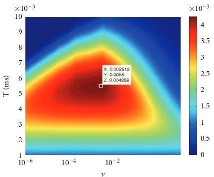
better for the design of low tracking threshold loops. For accelerations of 20 g fUFA(ν,T,a) is plotted in Figure15as
an example. It can be seen that the larger values of fUFAare
found in the region ofT near 5 ms and 10−4 < ν < 10−2,
and the maximum is approximately atν=0.0025 andT =
5.5 ms. The value of fUFA in this region is about 0.004. In
this case, the optimum loop bandwidth is aboutBN =70 Hz,
which is a more reasonable value than in the case of the PLL. For the UFA-PLL, the minimum pull-out probability and minimum output variance seem not to be as contradictory criteria as for the PLL. This can be understood noticing that the ability of the UFA-PLL for tracking in high dynamics depends on the smoothness of the transient error response rather than its absolute value, and then the output noise contribution becomes more relevant. Another important fact that must be emphasized is that even for 20 g accelerations it is not advisable to use correlation timesTlower than 5 ms.
Notice that, as it was explained in Section 2, this probability analysis applies also for an FLL as long as the right
[image:10.600.322.537.70.248.2] [image:10.600.56.284.71.232.2]26 28 30 32 34 36 38
Simulated Approximated
10−12
10−10
10−8
10−6
10−4
10−2
100
C/N0(dB/Hz)
P
rob
. non linear (PLL)
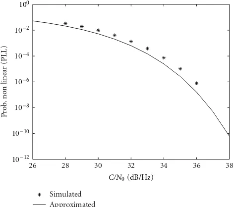
Figure16: Probability of NL behavior for type 3 PLL and 5 g.
4.3. Simulations. In this section we assess the accuracy of
the approximations made in the previous analysis. According to them the filter design of Section 3 is almost optimum when used in a UFA-PLL for tracking steps of 20 g, that is, it produces the minimum tracking threshold. The loop evolution with input noise according to a givenC/N0 was
simulated until the transient peak instant. Runs entering the nonlinear region before this peak were discarded. A variable number of runs were used in order to reduce simulation time as much as possible but keeping statistical significance of the results. Specifically, 100,000 runs were enough for the lowestC/N0values, whereas 100 million had to be used for
the highest.
A step of 5 g is considered in the simulation of the PLL, which produces a transient peak ofKp5 g (5 ms)2 = 1 rad.
Using (26) we found fPLL = 0.0033. The results of the
simulations compared with expression (25) are presented in Figure16. It can be seen that the approximation is slightly optimistic and that the error is almost constant in the simulated range ofC/N0. For the UFA-PLL we adopt a step of
20 g that produces a transient peak ofKp20 g (5 ms)2=2 rad
andKu20 g (5 ms)2=0.38 rad of peak difference. Using (25),
we getfUFA=0.004. The results of the simulations compared
with expression (31) are shown in Figure 17. In this case the approximation is still acceptable for tracking threshold determination, but now it is pessimistic and the error grows for increasing values of C/N0. This behavior is caused by
the Gaussian approximation that neglects the quadratic noise terms in the probability expression (28).
4.4. Tracking Threshold Analysis. To illustrate how this
anal-ysis can lead to loop designs with lower tracking thresholds we consider the design of a type 3 UFA-PLL for 20 g acceleration steps. The tracking threshold is determined by a given probability of pull-out, and then we will define it by a given level of probability of starting a nonlinear behavior.
26 28 30 32 34 36 38
Simulated Approximated
10−7
10−6
10−5
10−4
10−3
10−2
10−1
C/N0(dB/Hz)
P
rob
. non linear (UF
A)
Figure17: Probability of NL behavior for type 3 UFA-PLL and 20 g.
Therefore, if P is the admissible pull-out probability and
C/N0|THis the tracking threshold, then
PU≈Q
C
N0
TH
fUFA(ν,T)
=P, (33)
or equivalently,
C
N0
TH≈
Q−1(P)2
fUFA(ν,T). (34)
Clearly, minimum tracking threshold values will be achieved when fUFA(ν,T) is near its maximum, that is, using ν ≈
0.00025 and T ≈ 5.5 ms. Considering ν = 0.0003 and
T=5 ms, for example, the loop parameters areBN =80 Hz,
B′
N = 51 HzKpaT2 =2,KuaT2 =0.38, and fUFA =0.004.
Taking for instance a value of P = 0.001 and replacing in (34), we find thatC/N0|TH≈34 dB/Hz.
Another design, similar to those based on analog proto-types, can useν=0.000001 andT =2 ms and thenBNT =
0.1. The loop parameters becomeBN =50 Hz,B′N =13 Hz KpaT2 = 1.4, KuaT2 = 0.1, and fUFA = 0.002. Hence,
for the sameP = 0.001 if we replace in (34) the tracking threshold results C/N0|TH ≈ 37 dB/Hz. Therefore, the use
of the digital design method together with the proposed pull-out probability analysis can lower 3 dB the tracking threshold compared with traditional analog-based designs. An additional advantage is the use of longer values of T, requiring less computational load than analog designs.
It has to be mentioned that, even though the actual probability distribution can be different because of the Gaussian approximation, only the arguments of the Q(·)
are used in the comparison of both designs. Therefore, the comparison is not affected by the Gaussian approximation, that is, a modifiedQ(·) function could be used for a more
[image:11.600.311.546.73.284.2] [image:11.600.53.290.74.283.2] [image:11.600.317.547.349.430.2]5. Optimal Smoothing of the Phase Estimates
Due to the presence of two delays in the loop, the phase estimate obtained at a given instant is not computed with measurements up to this instant, but with measurements up to two previous instants. Thus, in the notation of [30] the loop phase estimate at the feedback branch is actuallyφ[i|
i−2]=φi. Naturally, the use of “closer” measurements would
produce a smoothing effect, that is, a better estimation. The real-time constraint does not allow taking advantage of this for the loop itself, but it is possible for other purposes as data detection and raw data generation for the navigation processes of the GNSS receivers. In this case, the optimal phase estimate can be obtained in the same way as before, but without forcing the two delays as in (9).
5.1. One Sample Smoothing. In this case the problem is
equivalent to obtaining the optimal loop filter with only one delay. Then, ifF′(z) is the new loop-filter transfer function
to be found, the corresponding closed loop transfer function is
T′(z)= F′(z)z−1
1 +F′(z)z−1 =Y
′(z)z−1, (35)
where Y′(z) is the rational and stable transfer function to
be found minimizing J(Y′(z)) in (8). Following the same
optimization process done in the AppendixA, the result is
Y′(z)=X′(z)z
Ψ(z) , (36)
where Ψ(z) is the same minimum phase rational function of (11) andX′(z) is the rational and stable transfer function
obtained from
G′(z)=γ2φ(z)φ
z−1
ψ(z−1) =X
′(z) +W′z−1. (37)
Noting thatG′(z)= G(z)/z, it is simple to relateX′(z)
with X(z) since the only change needed is to extract the possible pole inz=0 ofW(z−1)/zto obtainW′(z−1). Hence,
X′(z)= X(z)
z +
(G(0)−X(0))
z (38)
sinceW(z−1)=G(z)
−X(z). For the case we are interested
in, which is tracking of acceleration steps, according to (16)
G(0)=0. Then,
X′(z)=X(z)−X(0)
z , (39)
Therefore, the new optimum close-loop transfer function of (36) is
Y′(z)= C+ (A−3C)z−1+ (3C−B)z−2
(1−z1z−1)(1−z2z−1)(1−z3z−1), (40)
and the corresponding optimum loop filter is now only the three poles of the input,
F′(z)=C+ (A−3C)z−1+ (3C−B)z−2
(1−z−1)3
. (41)
Even more interesting is the expression of (36) in terms of the cascade of accumulators,
Y′(z)= p3+
p2−p31−z−1
+p1−p21−z−1
2
(1−z1z−1)(1−z2z−1)(1−z3z−1) ,
(42) If it could be possible to implement this loop filter, the feedback of the complete loop would beφ[i|i−1]. Of course
T′(z) = Y′(z)z−1 cannot be implemented with a real-time
loop, which has two delays, butY′(z)z−2can. Indeed, if the
loop filter structure of the UFA-PLL is slightly modified as shown in Figure 18, it can be shown that amazingly φ[i |
i−1]=xi(1)−xi(2). Clearly, the delay on the feedback branch
precludes the use of this value for the loop, but not for the rest of the GNSS receiver.
5.2. Two Samples Smoothing. The previous process can be
applied again. Now, the problem is equivalent to obtaining the optimal loop filter without delay. Then, ifF′′(z) is the
loop-filter transfer function and the corresponding closed loop transfer function is
T′′(z)= F′′(z)z−1
1 +F′′(z)=Y
′′(z), (43)
whereY′′(z) is the rational and stable transfer function to be
found minimizingJ(Y′′(z)) in (8) and replicating (36)–(39),
we obtain
X′′(z)=X′(z)−X′(0)
z . (44)
Therefore, the optimum transfer function of (43) is
Y′′(z)= p3+P2
1−z−1
+P11−z−1
2
(1−z1z−1)(1−z2z−1)(1−z3z−1), (45)
where P2 = (p2−2p3) andP1 = (p1 −2p2 −p3). Now T′′(z) = Y′′(z) cannot be implemented with a real-time
loop, butY′′(z)z−2 can. Again, based on the loop structure
of Figure18it can be shown thatφ[i|i]=xi(1)+1−2x(2)i+1+x(3)i+1.
5.3. More Samples Smoothing. As it was previously
men-tioned, sinceG(z) in (16) has four zeros atz =0 for inputs modeled as accelerations steps, the previous smoothing procedure can be done two more times. In this way, if some latency is allowed, the following phase estimates can be obtained based only on the real-time tracking loop of Figure18—the first three equations are repeated for clarity:
φ[i|i−2] =xi(1)−1,
φ[i|i−1]=x
(1)
i −x
(2)
i ,
φ[i|i]=xi(1)+1−2x(2)i+1+x
(3)
i+1,
φ[i|i+ 1]=x(1)i+2 −3x
(2)
i+2+ 3x (3)
i+2,
φ[i|i+ 2]=x(1)i+3 −4x(2)i+3+ 6xi(3)+3.
φi+nφi
^
φi
z−1
z−1
[·]π ei
1 1+Cz−1
+
+ + +
+
+
+ +
p3
p2
p1
1
1−z−1 1−1z−1 1−1z−1
UFA
−
ui x(3)i x(2)i xi(1)
Figure18: Block diagram of the UFA-PLL model with loop filter structure modified for phase smoothing.
These phase estimates can be interpreted as a prediction in the context of estimation theory [30]. In fact,φ[i|i−2]=
xi(1)−1can be obtained by propagatingφ[i−2|i−2] with the
signal dynamic model adopted for the phase estimation. If we considerxi=[x(1)i x
(2)
i x
(3)
i ] as the state of the loop input
phase model, the transition matrix must be
A=
⎡ ⎢ ⎢ ⎢ ⎣
1 1 1 0 1 1 0 0 1
⎤ ⎥ ⎥ ⎥
⎦. (47)
Since xi−1 include measurements up to the instant (i−2),
φ[i−2|i−2] can be found propagating backwards this state
as{A−2x
i−1}
(1). Notice that using this backward propagation
process with the matrixA−1, all the estimators of (46) can
be obtained. Actually, more smoothed estimates can be built. For example, the equation
φ[i|i+ 3]=xi(1)+4−5x(2)i+4+ 10x
(3)
i+4 (48)
can be used, but it is not optimal. As it will be shown in the simulations it can be considered useful because of its extremely simple implementation. In some way, the quantity of zeros in (16) atz = 0 gives a measure of the backward propagation capacity of the states estimated by the loop filter.
5.4. Simulations. The simulated loop model is a UFA-PLL
as shown in Figure 18 with the same filter coefficients of Section 3. The phase estimation error for an acceleration step of 50 g (starting at i = 5 and without noise) for the different estimators is plotted in Figure19. In this situation the loop error grows up to almost one cycle and therefore the data detection during this transient will not be possible. However, applying the smoothing process described by (46) the transient error is consistently reduced each time that a new input sample is used for the estimation. The response of the suboptimal estimator of (48) is also shown. It can be seen that its transient response is slightly worse than the obtained withφ[i|i+ 2].
The smoothing process also produces a decrease of the estimation noise variance. In Figure 20 the standard deviation of the six previous phase estimators is plotted for three different signal levels. These results were obtained simulating a linearized loop fed with Gaussian noise of variance 1/(2TC/N0). As expected, an increase of 3 dB in
the signal corresponds to a reduction of approximately√2 in the standard deviation. It is also possible to verify that
0 10 20 30 40 50
0 0.2 0.4 0.6 0.8
Phase er
ro
r (cy
cles)
−0.2
i(samples)
Meas. up toi−2 Meas. up toi−1 Meas. up toi
Meas. up toi+ 1 Meas. up toi+ 2 Meas. up toi+ 3
Figure19: Phase estimation error during a step of 50 g.
the standard deviation for the loop output, that is, without smoothing, is equal toσφi = BN/(C/N0). This expression
gives values 15.75◦, 11.14◦, and 7.88◦when the values ofC/N 0
are 30, 33, and 36 dB/Hz, respectively.
6. RF Test Experiments
The FLL-assisted PLL and the UFA-PLL designed in Section3
[image:13.600.119.482.74.157.2] [image:13.600.315.542.193.409.2]0 1 2 3 4 5 2
4 6 8 10 12 14 16
Number of samples in the update
Phase standar
d de
vi
ation (deg
re
es)
C/N0=30 dB/Hz
C/N0=33 dB/Hz
C/N0=36 dB/Hz
Figure20: Phase estimation standard deviation.
deviation of ∆f corresponds to a λ · ∆f instantaneous velocity, whereλis the L1 wavelength). The selected carrier power was−113 dBm. Taking into account the noise of the 50Ω output resistance of the generator and a noise figure of approximately 8 dB of the RF front-end gives aC/N0 =
53 dB/Hz, which is a relatively high value for GNSS receivers. This value was selected to obtain low noise curves for a visual comparison with the simulated responses since the noise performance has been already characterized.
A test of 10 g acceleration steps is shown in Figure21, depicting the tracked frequency detrended by a linear fit that accounts for the local clock drift. The amplitude of the triangular waveform was increased gradually up to the desired value to avoid large frequency steps. The measured phase error response of the FLL-assisted PLL at the output of the phase discriminator in one of the steps is shown in Figure 22, the response of the UFA-PLL is the same. The simulated response of the loop (as in Figure8) is also displayed to appreciate that the implemented loop is properly characterized by our model.
The same experiment was performed for acceleration steps of 40 g. The phase error responses of the FLL-assisted PLL and the UFA-PLL are presented in Figures23 and24, respectively. In the case of Figure 23, the step presented is negative and therefore the phase response is upside down with respect to the simulation in Figure 9. Again, a fine agreement between the measurements with real laboratory generated signals and the simulations can be appreciated.
7. Conclusions
A new carrier tracking loop design method for real-time GNSS receivers has been presented, which is completely optimized from the perspective of the digital nature of the correlation measurements. An analysis of the phase and frequency discrimination ideas from this point of
10 20 30 40 50
0 100 200
Time (s)
Estimat
ed fr
equency (Hz)
−200 −100
Figure21: Tracked frequency during a 10 g test.
35.8 35.9 36 36.1 36.2 36.3 36.4
0 0.1 0.2
Time (s)
Phase er
ro
r (cy
cles)
Measured Simulated
−0.2 −0.1
Figure22: Measured phase error during a 10 g step.
view allowed us to choose optimum discriminators often discarded because of the complexity of their analog counter-parts. Also, the known structure of FLL-assisted PLL has been considerably improved leading to a carrier loop that operates normally in phase locked condition and in frequency locked condition if the dynamics become severe enough. The effect of coupling the FLL to the PLL is considered at the design stage allowing a fine control of the effective loop bandwidth. Moreover, this approach allowed us to develop the UFA algorithm that corrects the cycle ambiguities of measured phase errors using the frequency information exploited by an FLL. With this algorithm it was possible to conceive a PLL that has the same advantages of an FLL-assisted PLL but avoids cycle slips and yet is easy to implement.
[image:14.600.312.546.70.254.2] [image:14.600.60.286.71.292.2] [image:14.600.314.544.283.488.2]