NSME: A Framework for Network Worm
Modeling and Simulation
Siming Lin1, 2, Xueqi Cheng1
1 Software Lab, Institute of Computing Technology, Chinese Academy of Sciences, Beijing
2 Graduate School of the Chinese Academy of Sciences, Beijing linsiming@software.ict.ac.cn, cxq@ict.ac.cn
Abstract. Various worms have a devastating impact on Internet. Packet level network modeling and simulation has become an approach to find effective countermeasures against worm threat. However, current alternatives are not fit enough for this purpose. For instance, they mostly focus on the details of lower layers of the network so that the abstraction of application layer is very coarse. In our work, we propose a formal description of network and worm models, and define network virtualization levels to differentiate the expression capability of current alternatives. We then implement a framework, called NSME, based on NS2 for dedicated worm modeling and simulation with more details of application layer. We also analyze and compare the consequential overheads. The additional real-time characteristics and a worm simulation model are further discussed.
1
Introduction
Internet worms have become a serious threat to the Internet infrastructure and users. It is important to study worm behaviors in order to find the effective countermeasures. An ideal approach is to create a realistic mathematical model that allows behavior prediction in a closed form. But in fact it is impossible to create such a model because there are a number of random factors difficult to be introduced in. For example, the epidemic model [1] greatly simplifies the details of the networks and worms.
The alternatives of network modeling and simulation have been studied for many years. Some famous simulators/emulators, such as NS2 [5] and ModelNet [6], have come forth. In our work, according to the theory of automata and discrete event system, we propose a formal description of network and worm models. By defining the virtualization levels, we then find different alternatives of network modeling and simulation have different expression capability. As mentioned above, current worm related research is mainly based on existing network simulators. However, these simulators mostly focus on the details of lower layers of the network so that the functions of application layer are greatly simplified. In addition, it is possible that packet level worm simulation will degrade the performance of these simulators.
We have developed a framework, called Network Security Modeling Environment (NSME), based on NS2 for dedicated worm modeling and simulation. We remove some inherent structures in NS2, such as Agent, and add some new features, such as host TCP/IP protocol stack, IP address supporting and external interfaces. These features make our framework support realistic application layer logic and make it achieve stronger expression capability, which means that it can be used in all worm related research, such as propagation simulation, honeypot and IDS test.
The remainder of this paper is organized as follows. Section 2 provides information on packet level worm simulation by others. Section 3 formalizes the problem. Section 4 describes our implementation in detail. Section 5 analyzes the performance of NSME and shows a worm simulation model based on it. Section 6 gives some conclusions and future directions.
2
Related Work
At present, there is much related work on packet level worm simulation. Riley et al [2] implement a worm model propagating with TCP and UDP protocols by using the GTNetS simulator [7]. In their work, the entire design of the worm model depends closely on many inherent and excellent features of GTNetS. However, a lot of attack packets with random destination IP Address generated by this model trend to degrade the performance of the NIx–Vector routing mechanism of GTNetS. To solve this problem, they take some enhancements, such as Routing Proxy, NIx– Vector Aggregation and so on. They have successfully simulated more than 50,000 nodes without exploiting the parallel and distributed simulation features of GTNetS.
Another significant work in this field is made by Liljenstam et al [3]. They point out that worm simulation is a challenge to the scale and performance of packet level simulators. They extend the SSFNet simulator [8] to implement a mixed abstraction worm simulation model. In this work, they use both epidemic model and packet level network model consisting of BGP routers. A pseudo-protocol is used to link the two
parts. Although less accurate, this hybrid method can achieve a scale of 102~103
autonomous systems (ASes) under the assumption that one BGP router represents one AS.
to simulate 15,000 nodes on 8 machines. In this work, they extend a lightweight TCP protocol to simplify computing. In addition, they point out some advantages and disadvantages of PDNS for worm simulation.
We find that most simulators usually cannot support the expression of application logic. For instance, NS2 does not have the functions related with IP address. Its Agent structure makes it static and trivial to configure protocols and connections in Otcl [5], which means all behaviors in NS2 are semiautomatic. These even affect its emulation function. Our framework will solve these problems.
3
Problem Formalization
3.1 Network Model
Given that R is a set of routers in the network, H is a set of hosts, L is a set of point to point data links, and C is a set of shared data links, the network topology can
be defined as T=
(
R, L, ϕ)
, where ϕ: L→ ×R R represents the adjacent relationship.If both set H and set C are not empty, their partitions {H
and exist, which makes
, H , , H }
1 2 n
{C , C ,1 2 ,C }n ∀ ∈i [1, ]n , ∃ ∈r R ,LANi=
(
{ }
r ∪H ,C ,i iϕi)
M= Q, V, , , , q , FΣ Γ ϒ
Q ∈
form the completely connected graphs, where n is the number of LANs.
Furthermore, characteristics of discrete packets transmission in computer
networks are conform to the discrete event system (DEVS) [10]. Therefore,
according to the theory of automata and discrete event system, we can get the general representation of the network modeling alternatives. We define a structure:
(
0)
ķQ is a set of states;
, where:
ĸV is a set of functional nodes;
ĹΣ is a set of external events;
ĺΓ is a set of internal events;
Ļϒ is a set of transition functions, and
ļq0 is the initial state;
ĽF⊆Q is a set of termination states.
The elements in V denote the handlers. Therefore, V R . is the
set of packets caused by the interaction between M and the external. A list is used to deal with the internal events. The elements in the list can be represented as
. It means the internal event with value
H L C
⊆ ∪ ∪ ∪ Σ
(
λ, ,v t)
∈ Γ λ will be received and processedby at the time of t. The ability of M to generate a variety of simulated behaviors
vastly depends on its abundant transition functions, e.g.:
v
(
, , ,) (
,)
δext = 2 denotes that receiving the external event under the state
1 from at the time of t will lead to the state transition to q , and generate the
internal event e.
1
q p v t q e
v
)
q e t q E P
p
q 2
(
, ,) (
, ,δint1 1 1 = 2 denotes that receiving the internal event e1 under state 1
at the time of t will cause the state transition to q , and generate a set of internal
q
2
( )
( )
( )
: Q V Q
: Q Q
: Q Q
ext
int1
int2 δ δ δ
× Σ × × → × Γ
× Γ × → × Γ × Σ
× Γ → × Γ ×
⎛ ⎞
⎜ ⎟
⎜ ⎟
⎝ P P P ⎠
{
}
{ }
,
,
ext int1
int2
δ δ
δ
Σ ≠ ∅ ϒ =
Σ = ∅
events E and a set of external events P.
(
,) (
,δint2 q e1 1 = q E t2 ,1
)
denotes that receiving the internal event will cause thestate transition from to , and generate a set of internal events , with the time
going to .
1
e
1
q q2 E
1
t
In δint1 and δint2, the received event e1 should be the one in the event list with the
minimum t and it will be removed from the list after the state transition is completed.
In addition, whether Σ is empty determines the values and natures of the set of
transition functions ϒ. δint2 depends on the value of t in the event e1 to maintain a
simulation clock, so it is not constrained by the real-time condition, while δext and
δint1 meet the real-time constrains, which are:
1: ( )δ < δ
c rt t , where rt( )δ is the time after δ is executed,
(
λδ,v tδ,δ)
is the eventwith minimum in the event list after t δ is executed;
(
)
(
)
(
)
2:δint1 1, λ1, ,1 1 , = 2, ,
c q v t t q E P holds if and only if 0≤ − ≤t t1 ε, where t is the
current time and ε is the adjustment factor.
3.2 Virtualization Levels
For M=
(
Q, V, , , , q , FΣ Γ ϒ 0)
, we give the following 3 definitions:Definition 1: When V=R∪L and Σ ≠ ∅, M can create a network model in low virtualization level. The receivers of the internal events in the model are limited to the virtual routers and data links. That is, the model only simulates the communication network. The hosts are outside the model and interact with it.
Definition 2: When V=R∪ ∪ ∪H L C and Σ ≠ ∅ , M can create a network model in medium virtualization level. The receivers in the model are extended to all
layers of the network. Furthermore, since Σ is not empty, the model must support
the communication between the external hosts and the internal virtual hosts.
Definition 3: When V⊆R∪ ∪ ∪H L C and Σ = ∅ , M will create a network
model in high virtualization level. Since Σ is empty, the model implements full
abstraction from physical data link, routing mechanism to data generation and response. Thus, it is a closure system.
The existing alternatives usually can only create models in one of the virtualization levels. The network emulators, such as ModelNet and Netbed [11], can reach low virtualization level. The network simulators, such as NS2 and SSFNet, can reach high virtualization level. The medium virtualization level is rigorous but less useful for traditional network research. Only few emulators, such as IP-TNE [12], can reach it.
It is significant for worm related research to get models in both high and medium virtualization levels. Using a high level model, the worm propagation can be simulated, and using a medium level model, living honeypot [13], another countermeasure against worms, can be constructed.
3.3 Behaviors of Worm-Daemon
(el,1,{el})
(ε,1-pv,Φ)
(ε, pv,{eu})
(ea,1,{el,er,es})
(el,1,{ea,ei,el})
(eu,pu,Φ)
qw0
qr
qv
ql
qi (es,ps,Φ)
(es,ps,Φ)
(ei,1,{ea,ei})
(er,pr,{eu})
(er,pr,{eu})
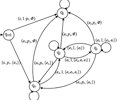
Fig. 1. The state transition graph of a daemon
worm propagation is to run a virtual daemon, which can simulate how a host
interacts with the worms. We define the daemon as
(
Q , H, w Γw,δw,qw0)
, where:ķQ 0 s v h is a set of states;
ĸH is a set of hosts;
{q , q , q , q , q } =
w w i
ĹΓ ⊂w Γ is a set of internal events;
ĺδw is similar to δint2 , but there is an probability parameter prob in it.
(
, ,) (
, ,)
δw q e prob1 1 = q E t2 1 means it will happen with the probability prob that
receiving the internal event e1 under the state 1 will cause the state transition to ,
and generate a set of internal events , with the time going to t ;
q q2
E 1
Ļqw0 w is an initial state.
Let state qr denotes a robust host that cannot be infected by any worms; qv
represents a host with vulnerabilities; ql is the latent state after the host has been
infected; and is the propagating state. We can also define the following behaviors.
Q ∈
qi
A host is vulnerable with
the probability v and it can
be upgraded by patches to become a robust host with
the probability u . An
infected host can become a robust host by upgrading with the probability
p
p
s
p , or
resume the vulnerable state
with the probability r .
[image:5.612.271.473.247.421.2]Worms do not infect the same victims, and they alternate between the latent and propagating states. Based on these assumptions, Figure 1 shows the state transition graph of a worm-daemon.
p
4
Implementation
4.1 Topology and Event Scheduling
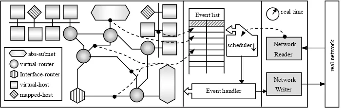
The topology basically consists of virtual hosts, virtual routers and related data links. In low or medium level models, the mapping hosts and interface routers can be additional used, acting as the interfaces between NSME model and the real network. Like a virtual host, an abstract subnet can handle all the data streams within a sub-network with a uniform protocol stack. By this way, it is flexible to control over the scale and the complexity.
Event handler virtual-host
mapped-host virtual-router Interface-router
abs-subnet
scheduler
real time
real network
Network Reader
[image:6.612.135.486.71.182.2]Network Writer Event list
Fig. 2. The architecture of the topology and the event scheduling in NSME framework
delay. Figure 2 shows the architecture of the topology and the event scheduling in NSME framework.
4.2 Communication Architecture
4.2.1 Packet and Routing
The packet headers in NSME follow the structures in the real network protocols instead of the inherent structures in NS2, such as ns_addr_t. Furthermore, in order to generate low or medium level models, the real data field has been supported. However, for generating high level models, the abstract packets are also used, which means the size of a packet can be greater than the sum of the actual size of its header and data field.
We use the classical algorithm, Dijkstra, to compute routes and implement a RadixTreeClassifier class which inherits from the NSObject class to perform IP packet forwarding. In this class, the routing table is constructed with realistic Radix tree structure. Therefore, it is available to allocate IP addresses and partition the network segments in the simulation model.
4.2.2 Protocol Stack
The major difference from NS2 is that each NSME virtual host has a mini but fully functional TCP/IP protocol stack. Therefore, the application layer is no longer a dispensable structure. Virtual application programs can gain the ability to access the network model via Virtual Sockets which replace NS2 Agents to process the protocols in lower layers. These sockets are no longer pre-configured, but controlled jointly by the protocol stack and virtual programs. The main benefit from this change is that virtual programs can directly use the real data and protocols to communicate without caring about whether the other end is a virtual host or an external real host.
complicated TCP connections are managed by both TCPListenSocket and TCPSocket. TCPSocket, derived from FullTCPAgent in NS2, provides the ability of flow control, packet assembly and retransmission. TCPListenSocket is used to manage passive connection requests. These socket classes are not associated with the Otcl classes. The developers do not need to care about the details of the connections and protocols. In a word, programming with Virtual Sockets in NSME is the same as writing a normal network program except that the Socket APIs are different.
Furthermore, ip_local_deliver is used to replace the old PortClassifier class to dispatch packets locally. Figure 3 shows the design of NSME protocol stack. It is easy to find our stack is quite similar to that in real systems (e.g. Linux). When a Virtual Socket is created, it will be registered on ip_local_deliver. When any packets arrive, ip_local_deliver will send them to rawip_filter for filtering. If an instance of RawSocket derived class is registered to intercept a certain protocol, rawip_filter will replicate the related packets and send them to it. Rawip_filter will also forward all packets to protocol handler entries
according to their protocol types, and the packets that are not matched will be discarded. Icmp_handler will directly process ICMP packets without forwarding them to the upper layers. However, tcp_demuxer and udp_demuxer are more complicated. They need to create quick indices for all the registered sockets. In addition, tcp_demuxer needs to distinguish active and passive connections. Our protocol stack can response UDP or TCP requests that are not matched by sending special packets, such as ICMP destination-unreachable packets and TCP RST packets. It will be also possible to imitate the stack fingerprint of a certain OS.
TCP socket
UDP socket raw socket TCP listen
socket tcp socket tcp socket create
ip_local_deliver
rawip_filter
in_point out_point
icmp_handler udp_demuxer
445 1322
tcp_demuxer
80 23
dport_BBTree 7240
sport_BBTree sip_BBTree 202.118.1.82
virtual socket layer
[image:7.612.282.483.241.467.2]dport_BBTree
Fig. 3. NSME protocol stack
virtual application logical layer
4.3 External Interfaces
between the real network and the model network.
We run NSME on host A with IP address 202.118.19.128, and there is another host B with IP address 202.118.19.132. First, we deploy two class C sub-networks (210.120.2.0, 202.118.19.0) connected by a virtual router into NSME model. Second, we allocate IP address 202.118.19.132 to a mapping host in this simulation model. Finally, we add a new routing entry to host B:
route add 210.120.2.0 mask 255.255.255.0 202.118.19.128
Now, host B has been partially mapped to the above mapping host so that it can communicate with the sub-network 210.120.2.0 in this model. However, it can still communicate with other real local hosts. We then add another routing entry to host B:
route add 202.118.19.0 mask 255.255.255.0 202.118.19.128
Now, host B is fully mapped into the simulated sub-networks (both 210.120.2.0 and 202.118.19.0), and can no longer communicate with other real local hosts, except host A.
5
Experiment and Analysis
In this section, we will analyze and compare the related overheads between our framework and NS2, then discuss real-time characteristics of our framework. Finally, we simulate a random scanning worm.
5.1 Routing Overheads
Figure 4 shows the comparison of the look-up time overhead (LTO) and basic memory overhead (BMO) between NSME routing and NS2 routing (The experimental hardware is a PC with a P4, 2.6GHz CPU and 4GB memory). On axel x, different scales of 1~10,000 are drawn in order to illuminate the issue of scale. It is easy to see that the LTO approximates a constant (0.96 us) in NS2. The BMO is about 2GB when it obtains the maximal scale of 5,000 nodes. The LTO and BMO in NSME are both close to those in NS2 when the number of nodes is less than or equal to 1,000. But the up-limit in NSME is 4,000 nodes with the LTO of 1.2 us and the BMO of about 2GB.
When greater than 1,000 nodes, BMO is very high either in NS2 or in NSME. The reason is that a routing table must be maintained for each router, whose space
complexity is O(n2). In NSME,
the routing table is implemented by Radix tree but not linear array, which makes the LTO and BMO are higher than those in NS2. Note that in this experiment, we only use virtual routers in NSME (for the ease of comparison). In fact virtual hosts do not need routing tables
in NSME, which makes it Fig. 4. Routing overheads
100 101 102
Nodes 10
3
100 104
102
101
BMO(
MB)
103
0.2 0.4 0.8
0.6
L
T
O
(us)
1.0 1.2 1.4
NSME (mm) NS2 (mm) NSME (time)
NS2 (time)
different from NS2.
5.2 Structure Overheads
With the same experimental hardware, we measure the overheads brought by the Virtual Socket structure in NSME and the Agent structure in NS2 respectively. Figure 5 shows both time and memory overheads when the TCP connections are
assigned in the phase of initialization. In NSME, two virtual hosts, Hv1 and Hv2, are
configured, and N (1≤N≤10, 000) virtual clients with TCP sockets on Hv1 are
assigned to prepare for connections to the virtual server on Hv2. Corresponsively, the
similar configuration is given in NS2, in which FullTcpAgents are used and the number of them is equal to that of virtual clients.
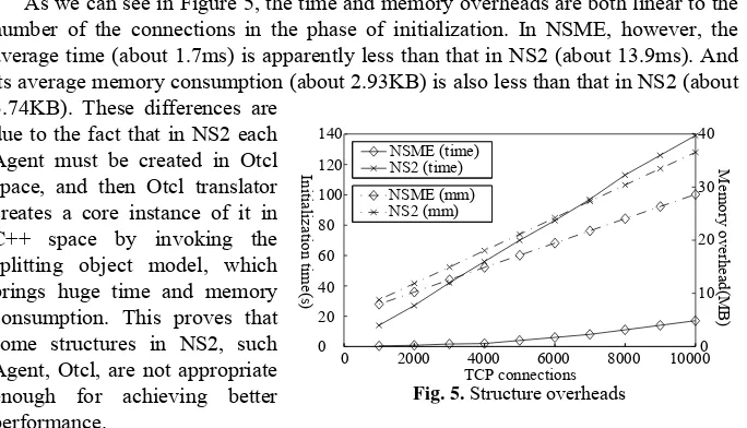
As we can see in Figure 5, the time and memory overheads are both linear to the number of the connections in the phase of initialization. In NSME, however, the average time (about 1.7ms) is apparently less than that in NS2 (about 13.9ms). And its average memory consumption (about 2.93KB) is also less than that in NS2 (about 3.74KB). These differences are
due to the fact that in NS2 each Agent must be created in Otcl space, and then Otcl translator creates a core instance of it in C++ space by invoking the splitting object model, which brings huge time and memory consumption. This proves that some structures in NS2, such Agent, Otcl, are not appropriate enough for achieving better performance.
10000 0
6000
[image:9.612.144.486.227.423.2]0 40002000 8000
Fig. 5. Structure overheads
TCP connections 140 100 60 40 80 Init ial iz ati on time( s) 120 20 40 30 20 10 Mem o ry ov er he ad (M B ) NSME (mm) NS2 (mm) NSME (time) NS2 (time) 0
5.3 Real-time Characteristics
We designed five scenarios in order to observe the real-time characteristics in
NSME. Scenario 1 includes a 1,000Mbps (0.1ms delay) LAN L1, where mapping
hosts Hs1, Hs2 and virtual host Hv1 are deployed. An additional LAN L2 exists in other
4 scenarios, where L1 and L2 are
connected through one-hop or ten-hop link(s) respectively, and the delay of each hop is 0.1ms or 1ms respectively (1,000Mbps bandwidth). In the 4 scenarios, the difference from scenario 1 is
that we deploy Hs1, Hs2 in L1 and
Hv1 in L2 (for medium
virtualization), or Hs1 in L1 and
Hs2 in L2 (for low virtualization).
10hops; 10ms 50 L o w virt ual iz ati o n (Mbps ) 40 10 20 30 120
100 0
[image:9.612.145.486.466.636.2]M u rt za ( p 60 Mb 10 tion 20 u ali 30 m vi 40 edi 50
Fig. 6. Real-time characteristics
The experimental environment consists of 3 PCs (P4 2.8GHz, 256M memory) in a
100Mbps LAN. Host A runs NSME and hosts B, C are mapped to Hs1, Hs2
respectively.
For medium virtualization, clients on hosts B and C request TCP connections to
server on Hv1. Each connection utilizes a timer to try to send data at 0.78Mbps. For
low virtualization, clients on hosts B and C communicate with each other. The solid line in Figure 6 illustrates the transmission rate of all the connections in medium virtualization level and the dashed line shows the situation in low virtualization level. We can see the rate increases linearly when the number of connections is less than 60, which means the good real-time performance. When the number of connections is more than 60, the performance drops if the number of hops increases. Meanwhile, the link delay affects the real-time performance. When the number of connections is greater than 80, the utility rate of CPU of host A generally drops to 90% and below, which means the performance of the network interfaces should be improved. In addition, since NSME model actually acts as a relay between host B and host C in low virtualization level, it is more sensitive to the bandwidth of the physical links and the performance of the network interfaces. Consequently, application layer can only achieve a lower transmission rate in this situation.
5.4 Worm Experiment
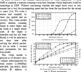
In order to observe the runtime characteristics of worm simulation, we used NSME to simulate a random scanning worm like Slammer which duplicates itself by transmitting in UDP. Without concerning whether the target hosts exist or not, Slammer has a very fast propagating speed and has been the top threat for the recent two years [14]. We write a
daemon and simplify its actions (no update and no recovery). This worm model exploits random scanning strategy to select target, and then sends it a single attack packet. If the target is vulnerable and has not been infected, it will be infected a short time later after receiving the attack packet. We list in table 1 several major parameters for this worm model.
This worm model is deployed to 10 abstract class B subnets interconnected by virtual routers (1,000Mbps bandwidth, 1ms delay). Each available IP address is
0 20 10 30 40 50 60 70 80
Simulation time (s) (a) Infected rate vs. Simulation time
90 100
20% 60 40% % 80% 100% s=5; w=100% s=5; w=70% s=10; w=70% s=5; w=100% s=5; w=70% s=10; w=70% s=5; w=100% s=5; w=70% s=10; w=70% 0 10 10 10 10 10 10 10 E vent s (p er si m-se co nd ) 3 6 108 100 1 2 4 5 7
20 50 90 70 80
10 30 40 60
[image:10.612.148.482.338.635.2]Simulation time (s) (b) Events (per sim-s) vs. Simulation time
Fig. 7. Worm experiment
100 10
occupied by a virtual host. The scanning strategy is random scanning in 226 addresses space. We find that the parameter t has no obvious effects on the propagation of the worm. The parameter i does affect the propagation, but it is not essential. Figure 7(a), where t=0.1s and i=1, illustrates the variation of the infection rate vs. simulation time brought by different s and w. Increasing either one will obviously aggravate the infection rate. In contrast to (a), figure 7(b) shows the relationship between NSME events (run time) and simulation time. It illustrates that the scan rate and weak degree will also affect the number of events which eventually determines the run time of the worm model. It is obvious that the large scale worm simulation will be a challenge to the discrete event simulators.
Table 1.Parameters for the worm experiment
Parameter Description
s the scan rate of the worm
w the weak degree which is a percentage of vulnerable hosts in a subnet
t the time delay when a host is infected
i the number of the initial infected hosts
6
Conclusion and Future Work
In this paper, we propose a formal description of network and worm models. We then implement the NSME framework based on NS2 for dedicated worm modeling and simulation. Our framework extends the details of the network modeling and simulation, so it is unavoidable to consume more memory and CPU time. Therefore, we must trade off between the accuracy and scale. In our worm model, we use abstract subnets to achieve large scale simulation, but it is not accurate. Furthermore, the flat routing mechanism is a bottleneck of the memory utility.
Our future work is to improve the scale and performance of the NSME framework. The approach mentioned in literature [15] is valuable for us. However, the technology of parallel and distributed simulation is essential to enhance the scale and performance, so we will focus on it. In this aspect, PDNS will be naturally compatible with our framework.
References
1. H. Andersson, T. Britton, and K. Krickeberg et al, Stochastic Epidemic Models
and Their Statistical Analysis, Springer-Verlag, New York, 2000
2. G. F. Riley, M. I. Sharif, and W Lee, “Simulating Internet Worms”, In
Proceedings of the 12th Annual International Symposium on Modeling, Analysis, and Simulation of Computer and Telecommunications Systems (MASCOTS'04), IEEE Computer Society, Washington DC, 2004, pp. 268-274
3. M. Liljenstam, Yougu Yuan, and BJ Premore, et al, “A Mixed Abstraction Level
the 10th IEEE Int'l Symp. on Modeling, Analysis and Simulation of Computer and Telecommunications Systems (MASCOTS'02), IEEE Computer Society, Washington DC, 2002, pp. 109-116
4. Anil Sewani, Bowei Du, “Packet Level Worm Simulation and Analysis”,
http://www.eecs.berkeley.edu/~anil/, 2004
5. L. Breslau, D. Estrin, and K. Fall, et al, “Advances in Network Simulation”, IEEE
Computer, 2000, pp. 59-67
6. A. Vahdat, K. Yocum, and K Walsh, et al, “Scalability and Accuracy in a
Large-Scale Network Emulator”, In Proceedings of the 5th Symposium on Operating Systems Design and Implementation, ACM Press, New York, 2002, pp. 271-284
7. G. F. Riley, “The Georgia Tech Network Simulator”, In Proceedings of the ACM
SIGCOMM workshop on Models, methods and tools for reproducible network research, 2003, pp. 5-12
8. SSFNet, “Scalable Simulation Framework Network Models”,
http://www.ssfnet.org/homePage.html, 1999
9. G. F. Riley, M. H. Ammar, and R. Fujimoto, “A Federated Approach to
Distributed Network Simulation”, ACM Transactions on Modeling and Computer Simulation, 2004, pp. 116-148
10.B P Zeigler, Theory of Modeling and Simulation, Wiley, New York, 1976
11.B. White, J. Lepreau, and L. Stoller, et al, “An Integrated Exerimental
Environment for Distributed Systems and Networks”, In Proceedings of the 5th Symposium on Operating Systems Design and Implementation, ACM Press, New York, 2002, pp. 255-270
12.R. Simmonds, R. Bradford, and B Unger, “Applying Parallel Discrete Event
Simulation to Network Emulation”, In Proceedings of the Fourteenth Workshop on Parallel and Distributed Simulation, IEEE Computer Society, Washington DC, 2000, pp. 15-22
13.I. Kuwatly, M. Sraj, and Z. A. Masri, et al, “A Dynamic Honeypot Design for
Intrusion Detection”, In Proceedings of the IEEE/ACS International Conference on Pervasive Services (ICPS'04). IEEE, 2004, pp. 95-104
14.Symantec Corporation, “Symantec Internet Security Threat Report”,
http://enter-prisesecurity.symantec.com, 2004
15.K. Walsh, E. G. Sirer, “Staged simulation: A General Technique for Improving