Cellular memetic algorithms evaluated on SAT

Cellular Memetic Algorithms Evaluated on SAT

Enrique Alba1_{, Bernab´e Dorronsoro}1_{, and Hugo Alfonso}2

1 _{University of M´alaga, Computer Science Dpt., M´alaga, Spain}

eat@lcc.uma.es; dorronsoro@uma.es

2 _{National University of La Pampa, General Pico, La Pampa, Argentina}

alfonsoh@ing.unlpam.edu.ar

Abstract. In this work, we study the behavior of several cellular memetic algorithms (cMAs) when solving the satisfiability problem (SAT). The proposed cMAs are the result of including hybridization techniques in dif-ferent structural ways into a canonical cellular genetic algorithm (cGA). Specifically, we hybridize our cGA with problem dependent recombination and mutation operators, as well as with three local search methods. Fur-thermore, two different policies for applying the local search methods are proposed. An adaptive fitness function (SAW), specifically designed for SAT, has been used for the evaluation of the individuals. Our conclusion is that the performance of the cGA is largely improved by these hybrid extensions. The accuracy and efficiency of the resulting cMAs are even better than those of the best existing heuristics for SAT in many cases.

1

Introduction

Evolutionary algorithms (EAs) are optimization techniques that work on a set (population) of potential solutions (individuals) by applying stochastic operators on them in order to search for an optimal solution. Most EAs use a single populati-on (panmixia) of individuals and apply operators populati-on them as a whole. In cpopulati-ontrast, there exists also some tradition in using structured EAs, where the population is decentralized somehow. Among the many types of structured algorithms, dis-tributed and cellular algorithms are two popular optimization tools [1, 2]. In many cases [3], these decentralized algorithms provide a better sampling of the search space, resulting in improved numerical behavior with respect to an equiv-alent algorithm in panmixia.

In the field of evolutionary computation, the latest advances clearly show that EAs can yield good results for SAT when hybridizing them with addi-tional techniques. Examples of these techniques are: adaptive fitness functions, problem-specific operators, local optimization, or parallel algorithms [8–11].

The motivation for this work is to study the behavior of different hybrid cGAs having generic or specific recombination, mutation and local search operators. We compare them against the basic local search heuristics themselves, and versus two canonical cGAs (without local search). Additionally, two different ways of embedding local search have been analyzed: (1) a computationally light local search step applied to every individual, or (2) an in depth exploitation local search step applied with a low probability.

This paper is organized as follows. In Section 2 we define the SAT problem. Section 3 introduces the studied algorithms, including three basic heuristics (GRAD, Simulated Annealing —SA— and WSAT), a basic cGA, and several cMAs, which are the result of different combinations with the previous algo-rithms. Our results are summarized in Section 4, and the conclusions and future research directions are addressed and discussed in Section 5.

2

Satisfiability Problems

The satisfiability problem (SAT) has received many attention from the scien-tific community since any NP problem can be translated into an equivalent SAT problem in polynomial time (Cook theorem) [12]; while the inverse transforma-tion may not always exist in polynomial time. This problem was the first which was demonstrated to belong to the NP class of problems.

The SAT problem consists in assigning values to a set ofnboolean variables x= (x₁, x₂, . . . , x_n) so that they satisfy a given set of clausesc₁(x), c₂(x), . . . ,

cm(x), wherec_i(x) is a disjunction of literals, and a literal is a variable or its negation. Hence, we can define SAT as a functionf :Bn_{→B, B={0,1}like:}

fSAT(x) =c₁(x)∧c₂(x)∧. . .∧c_m(x) . (1) An instance of SAT,x, is called satisfiable iff_SAT(x) = 1, and unsatisfiable otherwise. A k-SAT instance is composed of clauses with length k, and when

k≥3 (the cases we address in this work) the problem is NP-complete [13]. The fitness function we use is thestepwise adaptation of weights(SAW) [10]:

fSAW(x) =w₁·c₁(x) +. . .+w_m·c_m(x) . (2) This adaptive function weights the values of the clauses with wi ∈ N in

order to give more importance to those clauses which are still not satisfied by the current best solution. These weights are adjusted dynamically according to the formulawi =wi+ 1−ci(x∗), beingx∗the current fittest individual.

3

Canonical and Advanced Components in Cellular MAs

A detailed description of the algorithms used and first defined in this paper is given in the current section. Specifically, we study three simple heuristics for solving SAT (Subsection 3.1), a basic cGA —called JCell— (Subsection 3.2), and finally the proposed cMAs (Subsection 3.3).

3.1 Three Basic Local Search Techniques for SAT

In this subsection, we present the three local search procedures (LS) we have used for solving SAT. Two of them were specifically designed for this problem: (i) a gradient algorithm (GRAD), based on the flip heuristic, and especially developed for this work by the authors, and (ii) the well-known WSAT algorithm. The last procedure included is Simulated Annealing.

GRAD For the studies in this work, we have developed a new local search algo-rithm (GRAD) for SAT. GRAD is an algoalgo-rithm (based on the flip heuristic) that performs a gradient search in the space of solutions (see Algorithm 1). Basically, it consists in mutating the value of a variable according to the number of clauses it does not satisfy: the higher the number of unsatisfied clauses a variable belongs to, the higher the probability for mutating (flipping) it. As it can be seen in Al-gorithm 1, some noise is added to the search (with probability 0.2) in order to en-hance its exploration capabilities. The main difference of GRAD with respect to the flip heuristic consists in that the latter flips a variable (v) in terms of the gain of that flip:v={vi/max(sat clauses(vi)−sat clauses(vi))}(i= 1 to the number

of variables), while in GRAD the flip is made to every variable (v) satisfyingv= {vi/max(unsat clauses(vi))}with equal probability (independently of the gain).

This difference makes GRAD computationally lighter than the flip heuristic.

Algorithm 1Pseudocode of GRAD

1:GRAD(problem)

2:best ind =New Random Ind(); 3:while!Termination Condition()do 4: ind =New Random Ind(); 5: forsteps←0toMAX STEPSdo 6: ifrand0to1()<prob noisethen

7: Flip(ind,Random Variable Unsatisfying Any Clause()); 8: else

9: vars to flip[] =Variables Unsatisfying The Max Number Of Clauses(); 10: Flip With Equal Probability(ind, vars to flip);

11: end if

12: Evaluate Fitness(ind); 13: best ind =Best(ind, best ind); 14: end for

15: end while

unsatisfying the largest number of clauses— with equal probability (lines 9 and 10). With a preset probability (we use a value of 20%), some noise is introduced in the search. In this case, the offspring is obtained by flipping the value of a randomly chosen variable of the parent unsatisfying one or more clauses (lines 6 and 7). Then, the search process is repeated for the offspring (lines 5 to 14). Every MAX STEPS iterations the search is restarted —the current individual is randomly generated— (line 4). We have set this value to 10 times the number of variables. The algorithm stops (line 3) when the best-known solution is found or after making 2 millions of fitness function evaluations.

WSAT The WSAT algorithm [15] is a greedy heuristic also specifically designed for SAT. Basically, it consists in repeatedly selecting a non satisfied clause (ran-domly) and flipping one of its variables (see Algorithm 2). There exist some different methods for selecting this variable [16]. Among them, we have adopted the BEST strategy, which consists in flipping a variable of the clause with a given probability (prob noise = 0.5), or otherwise flips the variable that mini-mizes the number of clauses that are true in the current state, but that would become false (the clause) if the flip was made. After a number of steps, the search is “restarted” by replacing the current individual by a randomly generated one (line 3). Like in the case of GRAD, we have used 10 times the number of variables as the number of steps to “restart” (line 4), and the best so far found solution (the one with the largest fitness value) is always tracked.

Algorithm 2Pseudocode of WSAT

1:WSAT(problem)

2:best ind =New Random Ind(); 3:while!Termination Condition() do 4: ind =New Random Ind(); 5: forsteps←0toMAX STEPSdo

6: clause =Random Unsatisfied Clause() 7: ifrand0to1()<prob noisethen

8: Flip(ind,clause[randomInt(long clause)]); 9: else

10: fori←0tolong clausedo

11: lost clauses[i] =Broken Clauses After Flip(i);

12: end for

13: Flip(ind, clause[Index Of Min Value(lost clauses)]); 14: end if

15: Evaluate Fitness(ind); 16: best ind =Best(ind, best ind); 17: end for

18: end while

6 to 20). If the new individual is better (larger fitness value) than the best so far one it is accepted as the new best one (lines 14 and 15) and, otherwise, it replaces the best one with a given probability (lines 16 and 17). After some experimental tests, we have set the valuesTmax= 10,Tmin= 1, andcoolingRate= 0.8.

Algorithm 3Pseudocode of Simulated Annealing

1:Simulated Annealing(problem, Tmax, coolingRate)

2:ind =New Random Ind(); 3:best ind = ind;

4:while!Termination Condition() do 5: Temp = Tmax;

6: whileTemp>Tmindo

7: offspring = ind; // generate an offspring 8: fori←0 to problem.num varsdo

9: ifrand0to1()<1/problem.num varsthen 10: Flip(offspring,i);

11: end if

12: end for

13: Evaluate Fitness(offspring);

14: if Get Fitness(offspring)>=Get Fitness(ind)then 15: ind = offspring;

16: else ifrando0to1()< p(T emp, of f spring, ind)then 17: ind = offspring;

18: end if

19: Temp∗= coolingRate; 20: end while

21: best ind =Best(offspring, best ind); 22: end while

p(T emp, of f spr, ind) =e(Get Fitness(offspr)

−Get Fitness(ind))∗104

targetF itness∗T emp . (3)

3.2 The Cellular GA

Cellular GAs are a subclass of GAs in which the population is structured in a specified topology (usually a toroidal mesh of dimensions d = 1,2 or 3). In a cGA, the genetic operations may only take place in a small neighborhood of each individual (see Fig. 1). The pursued effect is to improve on the diversity and exploration capabilities of the algorithm (due to the presence of overlapped small neighborhoods) while still admitting an easy combination with local search at the level of each individual to improve on exploitation.

In this section, a detailed description of JCell is presented (see a pseudo-code in Algorithm 4). In JCell, the population is structured in a 2 dimensional toroidal grid, and a neighborhood of 5 individuals (NEWS) is defined on it (see Fig. 1). The algorithm iteratively considers as current each individual in the grid (line 3). An individual may only interact with individuals belonging to its neighborhood (line 4), so the parents selection is made among the individuals of the neigh-borhood (line 5) with a given criterion. Recombination and mutation genetic operators are applied to the individuals in lines 6 and 7, with probabilities Pc

andPm, respectively. After that, the algorithm computes the fitness value of the

offspring (line 8), and inserts it on the equivalent place of the current individual in the new (auxiliary) population (line 9) following a given replacement policy.

next generation (line 11) —this is called synchronous update. This loop is repea-ted until a termination condition is met (line 2), usually to reach the optimum, to make a maximum number of fitness evaluations, or a combination of they two.

Algorithm 4 Pseudocode for the canonical cGA 1: JCell(cga) //Algorithm parameters in ‘cga’

2: while !Termination Condition()do

3: forindividual←1tocga.popSizedo

4: _{n list =}Get Neighborhood(cga,position(individual));

5: parents =Selection(n list);

6: offspring =Recombination(cga.pc,parents);

7: _{offspring =}Mutation(cga.pm,offspring);

8: Evaluate Fitness(offspring);

9: Insert(position(individual),offspring,cga,aux pop);

10: end for

11: cga.pop = aux pop;

12: end while

Panmictic GA

Cellular GA

Fig. 1.Panmictic and cellular populations

3.3 Cellular Memetic Algorithms

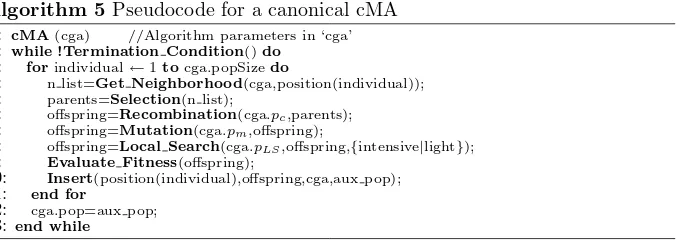
Memetic algorithms are evolutionary algorithms in which some knowledge of the problem is used by one or more operators. The objective is to improve the behavior of the original algorithm. Not only local search, but also restart, structured and intensive search is commonly considered in MAs[18]. In this work, we implement some cellular memetic algorithms (cMAs), obtained by hybridizing JCell with different combinations of generic and specific recombination, mutation and local search operators (see Table 1), as well as an adaptive fitness function specifically designed for SAT, SAW [10] (see Section 2). In Algorithm 5 we show the pseudocode for a canonical cMA. As it can be seen, the main difference between the pseudocodes of the canonical cMA and the canonical cGA is the local search step included in the cMA (line 8 in Algorithm 5).

Algorithm 5Pseudocode for a canonical cMA

1:cMA(cga) //Algorithm parameters in ‘cga’ 2:while !Termination Condition()do

3: forindividual←1tocga.popSizedo

4: n list=Get Neighborhood(cga,position(individual)); 5: parents=Selection(n list);

6: offspring=Recombination(cga.pc,parents);

7: offspring=Mutation(cga.pm,offspring);

8: offspring=Local Search(cga.pLS,offspring,{intensive|light});

9: Evaluate Fitness(offspring);

10: Insert(position(individual),offspring,cga,aux pop); 11: end for

12: cga.pop=aux pop; 13: end while

Table 1.Operators used to extend JCell to be a cMA.

Operator Generic Specific

Recombination DPX UCR

Mutation _{Binary UCM} Local Search SA GRAD

WSAT

Algorithm 6 Pseudocode for UCM

1: UCM(Indiv, Noise) 2: if rand0to1()≤Noisethen

3: Flip(Indiv, randomInt(Indiv.len)); 4: else

5: _MB(Indiv); 6: end if

keeping constant the values of the variables satisfying all the clauses they belong to. Our UCR is exactly the same operator asCB, and our UCM is the result of

adding some noise toMB, as it can be seen in Algorithm 5.

The three heuristics proposed in Section 3.1 have been adopted for being used as LS operators in JCell. As it can be seen in Section 4, some different configura-tions of these local search methods have been studied. These configuraconfigura-tions differ on the probability of applying the local search operator to the individuals and the intensity of the local search step. The idea is to regulate the overall compu-tational effort to solve the problem in affordable times with regular computers.

4

Results

In this section we analyze the results of our tests over the 12 instances (from

n= 30 to 100 variables) composing the suite 1 of the benchmark proposed in [9]. These instances belong to the SAT phase transition of difficulty, where hardest instances are located, since they verify thatm= 4.3∗n[19] (beingmthe number of clauses). The size of the problem is n= 30 for instances 1 to 3, n= 40 for 4 to 6,n= 50 for 7 to 9, andn= 100 variables for 10 to 12.

We test and compare the three proposed LS, as well as two basic cGAs in Section 4.1. After that, the behavior of the cMAs is analyzed in Section 4.2.

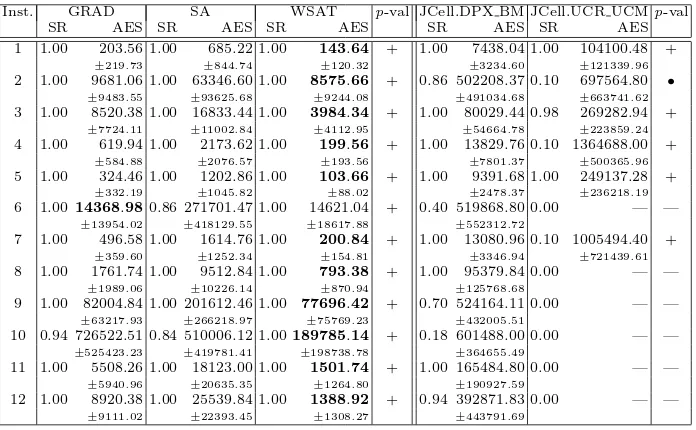
All the algorithms have been tested in terms of efficiency —Average number of Evaluations to Solution (AES)— and efficacy —Success Rate (SR)— (see tables 2 to 5). The results have been obtained after making 50 independent runs of the algorithms for every instance. We have computedp-values by performing ANOVA tests on our results in order to assess their statistical significance. A 0.05 level of significance is considered, and statistical significant differences are shown with symbol ‘+’ (‘•’ means non-significance) in tables 2 to 5.

4.1 Non Memetic Heuristics for SAT

In this section we study the behavior of GRAD, SA, and WSAT. Additionally, we test the behavior of two different cGAs without local search: JCell.DPX BM and JCell.UCR UCM. The former implements generic recombination and mutation operators (DPX and BM, respectively), while the latter has been hybridized with operators specifically designed for SAT (UCR and UCM). The parameters used in these cGAs are those of Table 3, but in this casepLS= 0.0 (there is no LS).

Table 2.Basic heuristics and metaheuristics.

Inst. GRAD SA WSAT p-val JCell.DPX BM JCell.UCR UCMp-val

SR AES SR AES SR AES SR AES SR AES

1 1.00 203.56 1.00 685.22 1.00 143.64 + 1.00 7438.04 1.00 104100.48 +

±219.73 ±844.74 ±120.32 ±3234.60 ±121339.96

2 1.00 9681.06 1.00 63346.60 1.00 8575.66 + 0.86 502208.37 0.10 697564.80 • ±9483.55 ±93625.68 ±9244.08 ±491034.68 ±663741.62

3 1.00 8520.38 1.00 16833.44 1.00 3984.34 + 1.00 80029.44 0.98 269282.94 +

±7724.11 ±11002.84 ±4112.95 ±54664.78 ±223859.24

4 1.00 619.94 1.00 2173.62 1.00 199.56 + 1.00 13829.76 0.10 1364688.00 +

±584.88 ±2076.57 ±193.56 ±7801.37 ±500365.96

5 1.00 324.46 1.00 1202.86 1.00 103.66 + 1.00 9391.68 1.00 249137.28 +

±332.19 ±1045.82 ±88.02 ±2478.37 ±236218.19

6 1.0014368.980.86 271701.47 1.00 14621.04 + 0.40 519868.80 0.00 — —

±13954.02 ±418129.55 ±18617.88 ±552312.72

7 1.00 496.58 1.00 1614.76 1.00 200.84 + 1.00 13080.96 0.10 1005494.40 +

±359.60 ±1252.34 ±154.81 ±3346.94 ±721439.61

8 1.00 1761.74 1.00 9512.84 1.00 793.38 + 1.00 95379.84 0.00 — —

±1989.06 ±10226.14 ±870.94 ±125768.68

9 1.00 82004.84 1.00 201612.46 1.00 77696.42 + 0.70 524164.11 0.00 — —

±63217.93 ±266218.97 ±75769.23 ±432005.51

10 0.94 726522.51 0.84 510006.12 1.00189785.14 + 0.18 601488.00 0.00 — —

±525423.23 ±419781.41 ±198738.78 ±364655.49

11 1.00 5508.26 1.00 18123.00 1.00 1501.74 + 1.00 165484.80 0.00 — —

±5940.96 ±20635.35 ±1264.80 ±190927.59

12 1.00 8920.38 1.00 25539.84 1.00 1388.92 + 0.94 392871.83 0.00 — —

±9111.02 ±22393.45 ±1308.27 ±443791.69

the problem in every run for all the instances. Conversely, in [20] WSAT only solved the problem in a 80% of the runs in the case of the largest instances (with

n= 100), so we have a better implementation of WSAT here.

Comparing the three basic LS, it can be seen in Table 2 that SA obtains the worst results, both in terms of efficacy and efficiency (with statistical confidence, except for instance number 10). GRAD is similar to WSAT in efficacy, but needs a larger number of fitness evaluations to find the solution (lower efficiency), except for instance 6 (significant values obtained in instances 3, 4, 7, 8, 10, 11, and 12). Hence, we can conclude that WSAT is the best one of the three heuristics for the studied test-suite, followed by GRAD. We also conclude on the superiority of problem dependent algorithms versus generic sheets of search like SA.

As a final conclusion, we can claim from Table 2 that the results of the two cGAs without explicit LS are always worse than those of the LS heuristics, both in terms of efficiency and efficacy. The best results of the table are those obtained by WSAT. Since we suspect that these results are too linked to the instances (specially to their “small” size) we will enlarge the test set at the end of the next section with harder instances.

4.2 Cellular Memetic Algorithms

In this section we study the behavior of a large number of cMAs with different parameterizations. As it can be seen in Table 3 (wherein details of the cMAs are given) we hybridize the two simpler cGAs of the previous section with three dis-tinct local search methods (GRAD, SA, and WSAT). These local search methods have been applied in two different ways: (i) executing an intense local search step (10×n fitness function evaluations) to the individuals with a low probability (calledintensive), or (ii) applying to all the individuals a light local search step, consisting in making 20 fitness function evaluations (called light).

Table 3.General parameterization for the studied cMAs

JCell.DPX BM+ JCell.DPX BM i+ JCell.UCR UCM+ JCell.UCR UCM i+

{GRAD,SA,WSAT} {GRAD,SA,WSAT} {GRAD,SA,WSAT} {GRAD,SA,WSAT} Local Search Light Intensive Light Intensive

pLS= 1.0 pLS= 1.0/popsize pLS= 1.0 pLS= 1.0/popsize

Mutation Bit-flip (pbf= 1/n),pm= 1.0 UCM,pm= 1.0

Recombination DPX,pc= 1.0 UCR,pc= 1.0

Pop. Size 144 Individuals Selection Current + Binary Tournament Replacement Replace if Better

Stop Condition Find a solution or achieve 100.000 generations

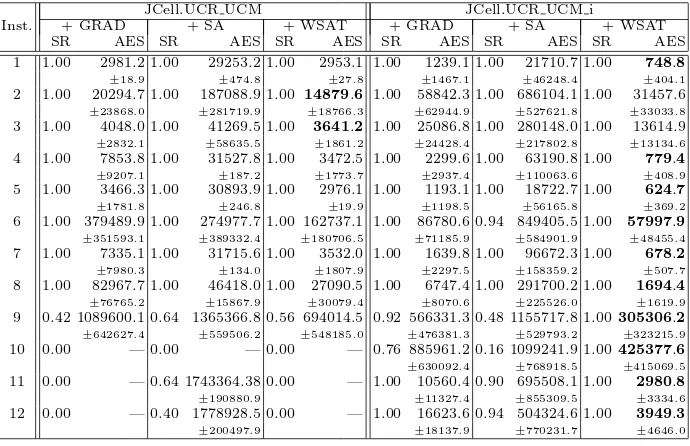
The results are shown in tables 4 and 5. If we compare these results with those of the cGAs in Table 2, we can see that the behavior of the algorithm is improved, in most cases, in efficiency and efficacy after including a local search step, specifically in the cases of GRAD and WSAT.

Comparing the studied cMAs in terms of the way the local search method is applied (intensive or light), we conclude that the intensive case always obtains better results than the light one when hybridizing the algorithm with one spe-cific heuristic (either GRAD or WSAT). Conversely, in the case of using SA, this is not always true, since the SA applied in an intensive way only outper-forms the other case in 9 out of the 24 tests. Again, specialized LS is preferable to generic LS. All these comparisons are statistically significant in 58 out of the 65 cases in which all the cMAs obtained the solution almost once.

Table 4.Results for the proposed hybridizations to JCell.DPX BM.

JCell.DPX BM JCell.DPX BM i

Inst. + GRAD + SA + WSAT + GRAD + SA + WSAT

SR AES SR AES SR AES SR AES SR AES SR AES

1 1.00 3054.2 1.00 29474.5 1.00 2966.1 1.00 1072.8 1.00 9649.6 1.00 569.9

±392.2 ±583.4 ±19.2 ±1112.6 ±25809.9 ±302.8

2 1.00 33598.7 1.00 195397.6 1.00 32730.4 1.00 50886.2 0.90 559464.3 1.00 30885.5

±51766.6 ±295646.3 ±49353.2 ±44167.7 ±437996.2 ±22768.8

3 1.00 14761.2 1.00 33005.4 1.00 4104.5 1.00 20385.8 1.00 255902.5 1.00 9418.4

±24935.1 ±6306.3 ±3325.1 ±20115.7 ±275734.7 ±10239.6

4 1.00 5018.6 1.00 31618.8 1.00 3972.9 1.00 2573.4 1.00 49310.9 1.00 794.7

±2397.8 ±152.9 ±1343.8 ±2497.7 ±64714.9 ±693.7

5 1.00 3575.6 1.00 31052.9 1.00 3008.3 1.00 1586.0 1.00 13354.0 1.00 628.6

±1131.5 ±282.7 ±8.4 ±1757.9 ±36668.5 ±437.9

6 0.96 181863.6 0.96 434235.9 1.00 81966.1 1.00 94046.4 0.72 654160.4 1.00 41619.4

±343020.8 ±519011.4 ±114950.0 ±114105.9 ±476411.6 ±47466.8

7 1.00 5945.8 1.00 33621.6 1.00 4822.6 1.00 2342.6 1.00 37446.4 1.00 850.8

±2416.8 ±7313.2 ±1364.9 ±2972.9 ±70165.5 ±527.5

8 1.00 14930.8 1.00 47688.6 1.00 7138.3 1.00 5164.5 1.00 195816.2 1.00 2097.6

±7644.5 ±15925.1 ±3957.5 ±5786.7 ±155018.9 ±1886.8

9 0.80 787149.2 0.50 720491.5 1.00 600993.9 0.82 963177.2 0.34 883967.7 1.00187814.5

±528237.4 ±597642.6 ±443475.3 ±585320.7 ±633307.9 ±148264.1

10 0.06 797880.3 0.04 1209394.0 0.06 1189559.7 0.04 1302489.0 0.10 1363627.4 0.80792051.2

±824831.9 ±90058.5 ±374193.7 ±346149.9 ±368403.3 ±491548.4

11 1.00 58591.3 1.00 1039910.2 1.00 35571.0 1.00 12539.8 1.00 357207.9 1.00 2466.3

±18897.3 ±205127.9 ±9243.6 ±10851.1 ±422288.9 ±1846.4

12 0.96 70324.9 0.98 1051351.2 1.00 45950.2 1.00 20018.2 0.98 409492.6 1.00 3196.9

±32808.8 ±174510.4 ±19870.7 ±19674.3 ±425872.3 ±2938.3

Table 5.Results for the proposed hybridizations to JCell.UCR UCM.

JCell.UCR UCM JCell.UCR UCM i

Inst. + GRAD + SA + WSAT + GRAD + SA + WSAT

SR AES SR AES SR AES SR AES SR AES SR AES

1 1.00 2981.2 1.00 29253.2 1.00 2953.1 1.00 1239.1 1.00 21710.7 1.00 748.8

±18.9 ±474.8 ±27.8 ±1467.1 ±46248.4 ±404.1

2 1.00 20294.7 1.00 187088.9 1.00 14879.6 1.00 58842.3 1.00 686104.1 1.00 31457.6

±23868.0 ±281719.9 ±18766.3 ±62944.9 ±527621.8 ±33033.8

3 1.00 4048.0 1.00 41269.5 1.00 3641.2 1.00 25086.8 1.00 280148.0 1.00 13614.9

±2832.1 ±58635.5 ±1861.2 ±24428.4 ±217802.8 ±13134.6

4 1.00 7853.8 1.00 31527.8 1.00 3472.5 1.00 2299.6 1.00 63190.8 1.00 779.4

±9207.1 ±187.2 ±1773.7 ±2937.4 ±110063.6 ±408.9

5 1.00 3466.3 1.00 30893.9 1.00 2976.1 1.00 1193.1 1.00 18722.7 1.00 624.7

±1781.8 ±246.8 ±19.9 ±1198.5 ±56165.8 ±369.2

6 1.00 379489.9 1.00 274977.7 1.00 162737.1 1.00 86780.6 0.94 849405.5 1.00 57997.9

±351593.1 ±389332.4 ±180706.5 ±71185.9 ±584901.9 ±48455.4

7 1.00 7335.1 1.00 31715.6 1.00 3532.0 1.00 1639.8 1.00 96672.3 1.00 678.2

±7980.3 ±134.0 ±1807.9 ±2297.5 ±158359.2 ±507.7

8 1.00 82967.7 1.00 46418.0 1.00 27090.5 1.00 6747.4 1.00 291700.2 1.00 1694.4

±76765.2 ±15867.9 ±30079.4 ±8070.6 ±225526.0 ±1619.9

9 0.42 1089600.1 0.64 1365366.8 0.56 694014.5 0.92 566331.3 0.48 1155717.8 1.00305306.2

±642627.4 ±559506.2 ±548185.0 ±476381.3 ±529793.2 ±323215.9

10 0.00 — 0.00 — 0.00 — 0.76 885961.2 0.16 1099241.9 1.00425377.6

±630092.4 ±768918.5 ±415069.5

11 0.00 — 0.64 1743364.38 0.00 — 1.00 10560.4 0.90 695508.1 1.00 2980.8

±190880.9 ±11327.4 ±855309.5 ±3334.6

12 0.00 — 0.40 1778928.5 0.00 — 1.00 16623.6 0.94 504324.6 1.00 3949.3

±200497.9 ±18137.9 ±770231.7 ±4646.0

it can be seen, the two algorithms find the optimal solution in the 100% of the runs (SR=1.0 for every instance), but JCell.UCR UCM i+WSAT obtains worse (higher) results than WSAT in terms of AES (statistically significant differences for all the instances). Although we expected a hard comparison against the best algorithm in literature (WSAT), we got similar accuracy and slightly worse efficiency in our tests, and we suspected this holds only in the smaller instances. With this scenario, we decided to test these two algorithms with larger instan-ces in order to check if the cMA is able to outperform WSAT in harder problems. For that, we have selected the 50 instances of 150 variables from the suite 2 of the same benchmark [9] studied before, in addition to those reported in tables 4 and 5. JCell.UCR UCM i+WSAT solved the problem at least once (of 50 exe-cutions) in 26 out of the 50 instances composing the benchmark, while WSAT found the solution for the same 26 instances and 4 more ones (hit rate lower than 2% for these 4 instances). Hence, WSAT is able to find the optimum in a larger number of instances, but with an average hit rate of 38.24%, which is quite close to 36.52%, the value obtained by JCell.UCR UCM i+WSAT.

Moreover, the average solution found for this benchmark (the optimal solu-tion is 645 for all the instances) is 644.20 for JCell.UCR UCM i+WSAT and 643.00 for WSAT, so the cMA is more robust in accuracy than WSAT for this set of instances. Finally, if we compute the average AES for the instances solved (at least once) by the two algorithms we can see that the cMA (Average AES = 364,383.67) is in this case more efficient than WSAT (Average AES = 372,162.36).

5

Conclusions and Further Work

In this work we have compared the behavior of 3 LS methods, 2 basic cGAs and 12 cMAs on the 3-SAT problem. These cMAs are the result of hybridizing the two cGAs with the 3 LS, applied at different parameterizations reinforcing diversifica-tion or intensificadiversifica-tion. Two LS, WSAT and GRAD (this one specially developed in this work), are specifically targeted to SAT, while SA is a generic one.

We have seen that the results of the proposed basic cGAs (without local search) are far from those obtained by the three studied LS. After hybridizing these basic cGAs with a local search step, the resulting cMAs substantially improved the behavior of the original cGAs. Thus, the hybridization step helps the cMAs to avoid the local optima in which the simple cGAs get stuck. For smaller instances, the best of the tested cMAs (JCell.UCR UCM i+WSAT) is as accurate as the best reported algorithm (WSAT) but slightly less efficient.

After these results, we decided to study the behavior of WSAT and JCell.UCR UCM i+WSAT with a set of larger instances. The results confirm our expectations, since the cMA is more accurate and efficient than WSAT for these larger instances. However, our results contrast with those of Gottlieb et al., who concluded in [20] that “A preliminary experimental investigation of EAs for constraint satisfaction problems using both an adaptive fitness function (based onfSAW) and local search indicates that this combination is not beneficial”. We

As a future work it would be interesting to test some different parameterizati-ons on the cMAs in order to improve the obtained results. Additionally, the hybri-dization of improved models of cGAs (asynchronous, adaptive, . . . ) could lead to still better results. Finally, an interesting work should be testing the algorithms with larger instances of the problem, in order to confirm our conclusion that JCell.UCR UCM i+WSAT performs better than WSAT for hardest problems.

References

1. Cant´u-Paz, E.: Efficient and Accurate Parallel Genetic Algorithms. Volume 1 of Book Series on GAs and Evolutionary Computation. Kluwer (2000)

2. Alba, E., Tomassini, M.: Parallelism and evolutionary algorithms. IEEE Trans. on Evolutionary Computation6(2002) 443–462

3. Alba, E., Troya, J.: Improving Flexibility and Efficiency by Adding Parallelism to Genetic Algorithms. Statistics and Computing 12(2002) 91–114

4. Alba, E., Dorronsoro, B.: The exploration/exploitation tradeoff in dynamic cellular evolutionary algorithms.IEEE Trans. on Evolutionary Computation9(2005)126–142 5. Alba, E., Dorronsoro, B., Giacobini, M., Tomasini, M.: Decentralized Cellular Evo-lutionary Algorithms. In: Handbook of Bioinspired Algorithms and Applications, Chapter 7. CRC Press (2004) (to appear).

6. Kautz, H.A., Selman, B.: Planning as satisfiability. In: Proceedings of the Tenth European Conference on Artificial Intelligence (ECAI’92). (1992) 359–363 7. Reiter, R., Mackworth, A.: A logical framework for depiction and image

interpre-tation. Artifitial Intelligence41(3)(1989) 123–155

8. Gottlieb, J., Voss, N.: Improving the performance of EAs for the satisfiability problem by refining functions. In: PPSN V, Springer (1998) 755 – 764

9. B¨ack, T., Eiben, A., Vink, M.: A superior evolutionary algorithm for 3-SAT. In: 7th Conf. on Evolutionary Programming. Vol. 1477 of LNCS, Springer (1998) 125–136 10. Eiben, A., van der Hauw, J.: Solving 3-sat with adaptive genetic algorithms. In:

IEEE CEC97, IEEE Press (1997) 81–86

11. Rossi, C., Marchiori, E., Kok, J.N.: An adaptive evolutionary algorithm for the satisfiability problem. In: Symposium on Applied Computing. (2000) 463–469 12. Cook, S.: The complexity of theorem-proving procedures. In Proc. of the 3rd

Anual ACM Symp. on the Theory of Computing (1971) 151–158

13. Garey, M., Johnson, D.: Computers and Intractability: a Guide to the Theory of NP-completeness. Freeman, San Francisco, California (1979)

14. Gottlieb, J., Voss, N.: Representations, fitness functions and genetic operators for the satisfiability problem. In: Artificial Evolution. LNCS, Springer (1998) 55–68 15. Selman, B., Kautz, H., Cohen, B.: Noise strategies for improving local search. In:

22th Nat. Conf. on Artificial Intelligence, California, AAAI Press (1994) 337–343 16. McAllester, D., Selman, B., Kautz, H.: Evidence for invariants in local search. In:

14th Nat. Conf. on Artificial Intelligence, Providence, RI (1997) 321–326

17. Kirkpatrick, S., Gelatt, C., Vecchi, M.: Optimization by simulated annealing. Science4598(1983) 671–680

18. Moscato, P.: Memetic Algorithms. In: Handbook of Applied Optimization. Oxford University Press (2000)

19. Mitchell, D., Selman, B., Levesque, H.: Hard and easy distributions for SAT prob-lems. In: 10th Nat. Conf. on Artificial Intelligence, California (1992) 459–465 20. Gottlieb, J., Marchiori, E., Rossi, C.: Evolutionary algorithms for the satisfiability