GNSS-R as a source of opportunity for remote sensing of the cryosphere

6

A proper characterization of extensive ice masses, with high spatial and temporal reso-lution, is an important requirement in the determination of their impact on the Earth’s climate. The present dissertation has evaluated the use of reflected GNSS signals towards remote sensing of the cryosphere. Despite being tested for a wide variety of applications, this technique is rather novel and represents a low cost source of opportunity for the monitorization of ice masses in Polar environments, a task specially challenging to be done in situ due to extreme weather conditions.

The research described along this dissertation could be classified in two main blocks, each of them dedicated to analysis of a different type of ice extensions: thin –hundreds of centimeters– sea ice covers; and thick –hundreds of meters– dry snow accumulations (mostly located in Antarctica and interior of Greenland). In both cases, theoretical studies and models have been developed, and their applicability has been supported by the results obtained from in situ experimental campaigns. Dedicated comments for each part are given afterwards.

Overall, the work presented here constitutes a first step toward ancillary applications that might be relevant to a possible future PARIS space-based mission (Martín-Neira et al., 2011). Such a mission, currently at the feasibility assessment level, will possibly follow a near-polar orbit, which would densely sample the vast Arctic and Antarctic areas. As a first recommendation for future work, further investigation to get a more comprehensive extrapolation of these results to a spaceborne scenario would be required.

6

.

1

One of the most significant parameters used for sea ice classification is its thickness, which can be estimated with accurate altimetric measurement of the freeboard level. In addition, permittivity and roughness retrievals might play a key role towards the same general purpose of characterizing sea ice extensions. Different GNSS-R observables have been analyzed to estimate these parameters during an experimental field campaign in Disko Bay, Greenland, from November 2008until May2009. The main difficulties faced during the analysis of the data have been related to (1) geometry, since the low elevation range available provoked overlapping between direct and reflected signals and failure of the standard known models; (2) technical aspects, mainly due to problems with the RHCP-R antenna’s connector and strong presence of near-by multipath; and (3) lack of more detailed in-situ data with similar spatial resolution as the GNSS-R measurements.

summary,conclusions and future work

hinder the proper altimetric retrieval under the first approach, the second methodology achieves better performances. The time evolution of the phase-delay retrieved heights matches with an Arctic tide model. In addition, the results obtained with reflected GPS signals at different polarizations are consistent and their combination enables a continu-ous height retrieval for the whole campaign’s period. While the mean formal precision of the single-track (_∼1 km) estimates is_∼3 cm, the1-day averaged measurements show a RMS standard deviation of 15.4 cm. The slow evolution of the height retrievals (once corrected with the tide model) follows the variation of the ice surface temperature pro-vided by MODIS, which is a key parameter in the rate of growth of sea ice. In absence of a proper ground truth, the range of the available altimetric measurements from ICESat GLAS obtained during the last years in the experimental site has been compared with the GNSS-R estimates, and it agrees with our estimations. However, the lack of more detailed ice information such as density and thickness (for comparison) hindered the performance of a proper retrieval of this last parameter from the altimetric results. In addition, the penetration of the L-band signal through sea ice should be also determined, which requires accurate determination of its permittivity.

The retrieval of sea surface roughness has also followed two different approaches. The first one explores how the scattering redistributes the power along the GNSS-R wave-form by obtaining a secondary intermediate observable, called scatterometric delay, and then inferring from it a MSSestimation by means of a standard KGO-based

electromag-netic model. Despite that the general variation of the results obtained show a realistic pattern, with peaks during high winds (provided by QuikSCAT) in open waters and min-imums during presence of smoother sea ice, further empirical corrections are needed to reach the expected range ofMSSvalues according to previous experiments. We consider

that the reasons are the limitations of the standard electromagnetic models to reproduce GNSS-R waveforms at such low angles of elevation, together with the contamination of direct signal into the reflected waveforms. Compared against the ice form information provided by DMI’s ice charts, the resultantMSSretrievals reach their lowest values when

compact ice floes are present, forming then a smooth sea surface, while they significantly increase with presence of just ice growlers, where the roughness conditions are still im-posed by the wind/water interaction, and for consolidated fast ice, which provides a rougher reflecting surface due the continuous ice cracking forced by the ocean tides. The second method under analysis makes use of the variability of the interferometric phase, which contains altimetric information, to perform an estimation of the RMS of the sur-face height level (RMSH), a parameter often employed to characterize surface roughness. However, the results obtained show a strong dependency with the signal’s power level, which is also related to the dielectric characteristics of the reflecting surface, thus being unable to achieve the proper separability between permittivity and roughness.

As in the other cases, two methodologies have been tested to obtain reflectivity estima-tions linked to the dielectric properties (permittivity) of the ocean surface. Both of them exploit polarimetric observables, that is, combining RHCP and LHCP reflected signals to determine the presence and evolution of sea ice by means of the Fresnel reflection compo-nents. The first approach consists of measuring the polarimetric ratio of the peak power waveforms with opposed polarizations. The evolution of these results during presence of sea ice shows good agreement with ice concentration measurements obtained with vi-sual inspection from a local Arctic weather station, as well as with the same information

6.2 remote sensing of dry snow

provided by DMI’s ice charts. The sensitivity of this method depends on the elevation an-gle. Being the slant geometries of this experimental scenario closer to the Brewster angle, they are more sensitive to variations in permittivity. The second method takes the phase difference of these waveforms with opposed polarizations (POPI). This method should be independent of the elevation angle. Due to limitations in the receiver’s internal con-figuration, the phase values were affected by an undetermined offset. For this reason, the analysis has to be limited to comparisons against the polarimetric ratio along the same ground track. There is correspondence between the evolution of both retrievals, specially during their most significant variations (presumably due to water/ice transitions). How-ever, decorrelated fluctuation patterns are found when general high values are reached (due to presence of sea ice). Motivated by the possibility of interaction between reflec-tions from sea ice and sea water (due to penetration of the incident signal through ice), a simple interferometric approach has been tested without success, so further research is needed to maximize the outcome of the POPI observable.

The main novelty introduced in the GNSS-R remote sensing of sea ice have been the use of polarimetric measurements, both phase and power observables. Next step should be a series of aircraft experiments, choosing a ground-track with a variety of sea ice conditions; repeating the ground-track several times, at different altitudes; and with ancillary instrumentation to measure and contrast the same parameters that GNSS-R might be sensitive to (e.g. roughness, permittivity, altimetry). These instruments should be either on-board or ground-based as in-situ proves. The ancillary ground truth should be also used to improve the modeling of the signal: to introduce a realistic probability density functions for different sea-ice (we have been using Gaussian distributions with typical standard deviations as in the roughness of open waters); and to incorporate layer and even volumetric scattering models (sea-ice with snow coverage, with multi-layer salinity gradients or snow volumetric scattering). Such an experiment should help compiling the information required to extrapolate the results to space-based scenarios: geometries closer to nadir, and gauging the effects of the receiver’s altitude on, not only SNR, but also parameters related to coherence of the reflected signals.

6

.

2

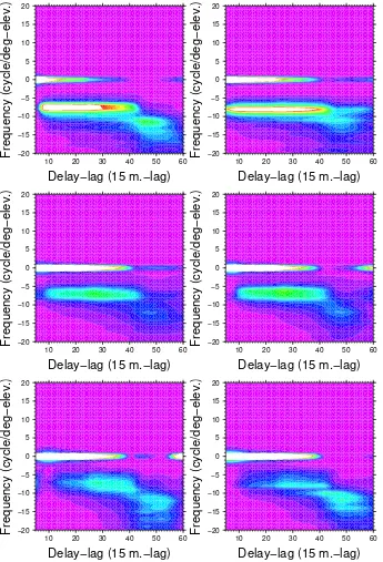
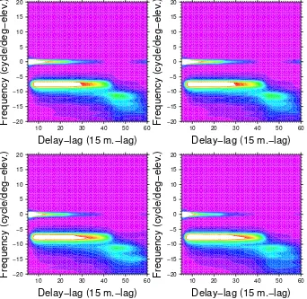
The interference fringes found in GNSS-R observables collected during an experimental field campaign at Dome Concordia, Antarctica, December 2009, cannot be explained by near-by multipath or external reflecting elements. In addition, the patterns show strong temporal repeatability. All indications point to reflections off internal layers of the snow as sources of these interference fringes. A simple model, Multiple-Ray Single-Reflection (MRSR), of L-band scattering and propagation through sub-surface layers of snow has been developed, and its qualitative agreement with the data is shown. The main conclusion is that the L-band GNSS signals penetrate into the snow, are reflected by some of its layers, and the reflected components interfere with each other and with the direct radio-link to generate the observed beating patterns. The depth of penetration is estimated to be down to 200-300meters, and a few of the layers are more reflecting than the rest.

summary,conclusions and future work

observables, that we have called lag-hologram. Further delayed lags of the waveform con-tain information about signal being more delayed with respect to the reference –direct– signal. Therefore, the complete lag-space must be inspected rather than just the peak of the signal, in order to obtain information from reflections occurring at deeper layers. While the lag-hologram identifies bright frequency stripes, the MRSR can also be used to link these frequencies into the depths of the reflecting layers that induced them. It has been shown that this translation is rather independent of inaccuracies in the a-priori snow density profile used by the model. The sole knowledge of the most reflecting layers might be of interest to complement L-band radiometric experiments, such as the space-borne SMOS and Aquarius missions. An example has been shown when comparing brightness temperature anomalies detected by a L-band radiometer placed in the same location with an adapted version of the MRSR. The fluctuation pattern found in the ra-diometric measurements has good agreement with the modeled signal coming from the Sun and reflected off the snow layers.

The attempts to invert real data into a complete layered permittivity profile by using a linearized approach have not been fruitful. In general, the solution strongly relates to the a-priori profile, even when loose covariances are given. The impression is that the real data lag-holograms present a set of high negative frequency bands in the central lags, which are not predicted by the model. It is unclear whether the model does not pre-dict them or it would, but these bands rest masked because it overestimates the surface reflection.

This study is pioneer in GNSS-R remote sensing of deep dry snow layers based on mul-tiple reflections. Despite the high temporal repeatability of the interferometric features found in the real data, the geographic consistency is rather low. Perhaps we are sensing inhomogeneities in the snow, but this has not been proven. Several other reasons that might explain this performance are contained in the validity of the model’s assumptions: locally horizontal snow layers, single layer-reflections and an homogeneous density pro-file for the entire area, _∼500 meter wide. All these assumptions should be carefully revised, and improvements in the model could be made to attempt more complete re-trievals of the snow sub-surface contents. For instance, estimates of the snow density or permittivity could be refined with the appropriate forward model; or tomographic ap-proaches implemented to solve for the3-D structures, including tilted layers and spatial inhomogeneities. Despite this limitation, the detection of the reflective layers can still be useful. As an example, in Hawley et al. (2006), the delays of radar measurements are not used to estimate the snow density, but combined with a given density profile to estimate the snow accumulation rates. A similar application can be envisaged for GNSS-R.

A

a

.

1

2SCM Two-Scale Composite Model

ALI Advanced Land Imager

ALOS Advanced Land Observing Satellite

AMSR-E Advanced Microwave Scanning Radiometer for EOS

AMSU Advanced Microwave Sounding Unit

AOTIM Arctic Ocean Tidal Inverse Model

ASAR Advanced Synthetic Aperture Radar

ASCAT Advanced Scatterometer

AVHRR Advanced Very High Resolution Radiometer

AWS Automatic Weather Station

BOC Binary Offset Carrier

BPSK Binary Phase Shift Keying

C/A-(code) Coarse/Acquisition (GPS code)

CDMA Code Division Multiple Access

CEOS Committee on Earth Observation Satellites

CHAMP Challenging Mini-satellite Payload

CoSMOS-OS Campaign on SMOS - Ocean Salinity

CSIC Consejo Superior de Investigaciones Científicas / Spanish

Re-search Council

DB Database

DDM Delay Doppler Map

DMC Disaster Monitoring Constellation

DMI Danmarks Meteorologiske Institut / Danish Meteorological

In-stitute

DMSP Defense Meteorological Satellite Program

DoD Department of Defense

DoY Day of Year

ECMWF European Centre for Medium-Range Weather Forecasts

ECV Essential Climate Variables

EGM96 Earth Gravitational Model1996

Envisat Environmental Satellite

EOS Earth Observing System

glossary of terms

ESA European Space Agency

ETM+ Enhanced Thematic Mapper Plus

FDMA Frequency Division Multiple Access

FFT Fast Fourier Transform

GCOS Global Climate Observing System

GEO Geostationary Orbit

GFZ GeoForschungsZentrum / German Research Centre for

Geo-sciences

GLAS Geoscience Laser Altimeter System

GLONASS Global’naya Navigatsionnaya Sputnikovaya Sistema / Global

Navigation Satellite System

GMES Global Monitoring for Environment and Security

GMF Global Mapping Function

GNSS Global Navigation Satellite Systems

GNSS-R Global Navigation Satellite Systems - Reflectometry

GOLD-RTR GPS Open Loop Real Time Receiver

GORS GNSS Occultation, Reflectometry and Scatterometry space

re-ceiver

GPS Global Positioning System

GPS-R Global Positioning System - Reflectometry

GPS-SIDS GPS - Sea Ice Dry Snow

GTOS Global Terrestrial Observing System

HH Horizontal-input to Horizontal-output polarization

HTTP Hypertext Transfer Protocol

HV Horizontal-input to Vertical-output polarization

ICE Institut de Ciències de l’Espai / Institute of Space Sciences

ICESat Ice, Cloud, and land Elevation Satellite

IEEC Institut d’Estudis Espacials de Catalunya / Institute for Space

Studies of Catalonia

IFAC Nello Carrara Istituto di Fisica Applicata / Institute of

Ap-plied Physics

IFREMER Institut Français de Recherche pour l’Exploitation de la Mer /

French Research Institute for Exploitation of the Sea

IGS International GNSS Service

IGSO Inclined Geosynchronous Orbit

INT Integrated Data (non-coherently at1sec)

IOV In-Orbit Validation (space vehicle)

IP Internet Protocol

IPCC Intergovernmental Panel on Climate Change

I&Q In-phase and Quadrature

KGO Kirchhoff approximation under Geometric Optics

KM Kirchhoff Method

LAN Local Area Network

LEO Low Earth Orbit

A.1 list of acronyms

LGGE Laboratoire de Glaciologie et Geophysique de

l’Environnement / Laboratory of Glaciology and Geophysics of the Environment at Grenoble

LHCP Left Hand Circular Polarization

LIDAR Light Detection And Ranging

LL LHCP-input to LHCP-output polarization

LNA Low Noise Amplifier

LR LHCP-input to RHCP-output polarization

M-(code) Military (GPS code)

MEO Medium Earth Orbit

MetOp Operational Meteorology

MIRAS Microwave Imaging Radiometer using Aperture Synthesis

MODIS Moderate-resolution Imaging Spectroradiometer

MRSR Multiple-Ray Single-Reflection model

MSS Mean Square Slope

MySQL My Structured Query Language

NASA National Aeronautics and Space Administration

NWPM Numerical Weather Prediction Model

NW-SE North-West to South-East

PALSAR Phased Array type L-band Synthetic Aperture Radar

PARIS Passive Reflectometry and Interferometry System

PDF Portable Document Format

POES Polar Operational Environmental Satellite

POPI POlarimetric Phase Interferometry

PRN Pseudorandom Noise (sequence)

P(Y)-(code) Encrypted Precise (GPS code)

QuikSCAT Quick Scatterometer

RA Radar Altimeter

RAW Raw Sampling Data (complex phasors at1msec)

RF Radio Frequency

RHCP Right Hand Circular Polarization

RL RHCP-input to LHCP-output polarization

RMS Root Mean Square

RR RHCP-input to RHCP-output polarization

RSS Residual Sum of Squares

Rx Receiver

SAR Synthetic Aperture Radar

SIRAL SAR/Interferometric Radar Altimeter

SMOS Soil Moisture Ocean Salinity satellite

SNR Signal to Noise Ratio

SPM Small Perturbation Method

SSA Small Slope Approximation

SSH Secure SHell

SSM/I Special Sensor Microwave/Imager

SSMI/S Special Sensor Microwave Imager/Sounder

glossary of terms

TanDEM-X TerraSAR-X add-on for Digital Elevation Measurement

TU Terminal Unit

Tx Transmitter

TZD Total Zenith Delay

UAV Unmanned Aerial Vehicle

UDP User Datagram Protocol

UE User End

UHF Ultra High Frequency

UK United Kingdom

UMTS Universal Mobile Telecommunications System

UTC Coordinated Universal Time

VH Vertical-input to Horizontal-output polarization

VLBI Very-Long-Baseline Interferometry

VV Vertical-input to Vertical-output polarization

WAV Woodward Ambiguity Function

WGS84 World Geodetic System1984

WIST Warehouse Inventory Search Tool

WMO World Meteorological Organization

WS Wind Scatterometer

ZHD Zenith Hydrostatic Delay

ZWD Zenith Wet Delay

A.2 list of symbols

a

.

2

A0 Illuminated area.

Ae f f Effective area of receiver antenna.

AM Multipath’s amplitude.

Ares Amplitude of the sawtooth wave that models the impact of

∆_Hin the variation of∆_φI.

AiS Distance between point Ai(wavefront reaching the surface for internal reflection at i-layer) and Specular reflection point in the MRSR model for dry snow remote sensing.

~_{b/[b] Vector/array of the inter-antenna baseline distance.}

B Receiver’s bandwidth.

BC/A =2.046 MHz Bandwidth of the GPS C/A signal.

c=299792458 m/s Speed of light in the free space.

C(t) Ranging code.

CC/A(t) C/A-code sequence.

CP(Y)(t) P(Y)-code sequence.

CI ≡Er·E∗_d Interferometric coherence-field.

Cpol = ERHCPr ·ELHCPr ∗ Polarimetric field.

C_W Data covariances for lag-hologram total inversion.

Cρ Model covariances for lag-hologram total inversion.

di One-way physical distance traveled inside the i-layer in the MRSR model for dry snow remote sensing.

D(t) Navigation data message.

Dhz Zenith hydrostatic delay.

Dwz Zenith wet delay.

Dz =Dhz+Dwz Total Zenith Delay (TZD).

Di Horizontal extent of the propagation inside the i-layer in the MRSR model for dry snow remote sensing.

e=2.7182818 Euler’s number.

~_e/_[e] Unit vector/array that defines the arrival direction of the sig-nal reflected at the specular point.

E0 Maximum amplitude of the incident electric field.

Einc Incident electric field towards the reflecting target.

Ed Direct field.

glossary of terms

Erpq Reflected electric field in the pq polarization state, i.e. p as input polarization andqas output polarization. If pandqare

the same polarization, the term co (co-polar) is employed; on

the other hand, when p and qare opposite polarizations, the

term cross (cross-polar) is used. In the case of GPS signals,

transmitted at RHCP polarization, Erco = ERHCPr and Erco =

ErLHCP.

~_Es

pq Scattered electric field in the pq polarization state, i.e. p as input polarization and qas output polarization.

E1 GNSS Frequency band between 1587.0 and 1591.0 MHz

em-ployed by Galileo and BeiDou-2/Compass. Some references define E1to the joint E2-L1-E1given here.

E2 GNSS Frequency band between 1559.0 and 1563.0 MHz

em-ployed by Galileo and BeiDou-2/Compass.

E5A GNSS Frequency band between 1164.0 and 1189.0 MHz

em-ployed by Galileo and BeiDou-2/Compass, overlapping with L5.

E5B GNSS Frequency band between 1189.0 and 1214.0 MHz

em-ployed by Galileo and BeiDou-2/Compass, overlapping with G3.

E6 GNSS Frequency band between 1260.0 and 1300.0 MHz

em-ployed by Galileo and BeiDou-2/Compass.

f(t) Carrier RF sinusoidal signal.

fI Interferometric frequency.

f_Isur f Interferometric frequency corresponding to the surface snow

level.

fL1 =1575.42 MHz GPS L1carrier frequency. fL2 =1227.60 MHz GPS L2carrier frequency. fL5 =1176.45 MHz GPS L5carrier frequency.

fM Multipath frequency relative to the main signal.

fL Linearized function for Lag-Hologram total inversion.

Feq Equivalent noise figure of the RF front-end.

FL Matrix of the partial derivatives of fL, numerically computed around the a-priori profileρsb.

FLN A LNA noise figure.

F {} Fast Fourier Transform.

Ga Antenna gain.

GLN A LNA gain.

Gr Receiver antenna gain (directivity).

Gt Transmitter antenna gain (directivity).

G1 GNSS Frequency band between 1593.0 and 1610.0 MHz

em-ployed by GLONASS.

A.2 list of symbols

G2 GNSS Frequency band between 1237.0 and 1254.0 MHz

em-ployed by GLONASS, overlapping with L2.

G3 GNSS Frequency band between 1189.0 and 1214.0 MHz

em-ployed by GLONASS, overlapping with E5B.

hscale=7160 m Scale height of the troposphere assumed during Greenland-dataset processing.

Hi Height (vertical width) of the i-layer in the MRSR model for dry snow remote sensing. In the case of i = 0 (air layer),

H0 corresponds to the height of the receiver’s antenna with

respect to the snow surface level.

HM Height of the receiver antenna above the multipath-reflector.

HR

S Vertical distance between receiver antenna and specular point of reflection.

H_ellipS Height of the surface with respect to the reference ellipsoid

WGS84(ellipsoidal height).

HMAX Ellipsoidal height retrieved using code-delay from maximum of the waveform.

HDER Ellipsoidal height retrieved using code-delay from maximum of the waveform’s first derivative.

HWGS84 Height between the reference ellipsoid WGS84and the sea ice

surface level.

Hsea Mean sea level with respect to WGS84.

i=√₋1 Imaginary unit.

Im{} Imaginary part.

k Wavenumber.

ki Wavenumber across the i-layer in the MRSR model for dry

snow remote sensing.

K=1.38_×10−23_{J/K Boltzmann’s constant.}

L Non-modeled losses in the radar equation (e.g. atmospheric

loss).

Lc Attenuation of the cable.

Lcorr Transversal correlation length of the reflecting surface.

L1 GNSS Frequency band between 1563.0 and 1587.0 MHz

em-ployed by GPS.

L2 GNSS Frequency band between 1215.0 and 1239.6 MHz

em-ployed by GPS, overlapping with G2.

L5 GNSS Frequency band between 1164.0 and 1189.0 MHz

glossary of terms

mv Volume fraction of liquid water in the snow mixture.

mhz Hydrostatic mapping function.

mwz Wet mapping function.

mss One-dimensional mean square slope.

MSS Two-dimensional mean square slope (or simply mean square

slope).

MSS0 A-priori mean square slope value for MSS-inversion.

n Refractive index.

ni Refractive index of thei-layer in the MRSR model for dry snow remote sensing.

ˆ

ns Normal scattered vector.

ˆ

ni Normal incident vector.

PC/AL1 Signal power for GPS signals carrying C/A-code on L1.

PP(Y)L1 Signal power for GPS signals carrying P(Y)-code on L1.

PP(Y)L2 Signal power for GPS signals carrying P(Y)-code on L2.

Pr Power sensed by the receiver antenna.

Pt Power transmitted.

P Probability Density Function of the surface slopes for a

Gaus-sian isotropic surface spectrum.

~_{q = (qx,qy,qz) ≡ k(n}ˆ_s−

ˆ

ni)

Scattering vector, perpendicular to the local tangent plane.

~_{q⊥= (qx},_qy) Components of~_qperpendicular to the incidence plane.

rcorr ≡ p

x2_corr+y2_corr Correlation radial distance.

Re f f Effective sampling rate.

R0 Distance from the point of observation (receiver) to the center of A0.

R1 Distance from transmitter to target.

R2 Distance from target to receiver.

Rd Electromagnetic path length of the direct signal.

Rr Electromagnetic path length of the reflected signal.

RMSφ Root mean square of the complex field’s phaseφI.

RMSH Contribution inRMSφfrom the residual height, related to

sur-face roughness.

RMSf ad/coh Contribution in RMSφ from the impact of random phase

de-partures produced by fading and coherence loss.

RMSmpath Contribution in RMSφ from distortion of the phase due to

multipath.

RMSN Contribution in RMSφ from instrumental noise.

RMSres Contribution in RMSφ due to the impact of an error in the

height estimation.

A.2 list of symbols

Rotx(θBF) Rotation matrix aroundx-axis in the local body-frame.

Roty(φBF) Rotation matrix aroundy-axis in the local body-frame.

Rotz(ψBF) Rotation matrix aroundz-axis in the local body-frame.

Re{} Real part.

ℜpq Fresnel coefficient in the pq polarization state, i.e. p as input polarization andq as output polarization. If p and q are the

same polarization, the termco (co-polar) is employed; on the

other hand, whenpandqare opposite polarizations, the term cross(cross-polar) is used.

ℜij Reflection Fresnel coefficient of a signal incident from

medium/layer i off the interface with medium/layer jin the

MRSR model for dry snow remote sensing.

~_r Spatial vector of the scattering points.

~_r′ Spatial vector required for integrating the different points across the reflecting surface.

s(t) Radar baseband signal.

sL1(t) GPS signal at L1(Blocks IIA and IIR). sL2(t) GPS signal at L2(Blocks IIA and IIR).

SC/A(κ)≡χC/A(0,κ) Frequency component ofχC/A forτ=0.

SC(p;pre f) Cost function that evaluates the overall difference between the lag-hologram resulting from a profile with a perturbation p, compared to a reference density profile with a perturbation

pre f.

t Time variable.

T Receiver temperature (antenna + thermal noise).

Ta Antenna temperature.

TLN A LNA temperature.

Tc Equivalent noise temperature of the cable.

Teq Equivalent noise temperature of the RF front-end.

Th Horizontal component of the brightness temperature.

Tv Vertical component of the brightness temperature.

Ti Coherent integration time.

TM =70 seconds Mean multipath period estimated during Greenland’s experi-mental campaign.

T_ENUNED Transformation matrix from a East-North-Up to a

glossary of terms

Tij Transmission Fresnel coefficient where the incident

layer/medium is i and the medium into which the

sig-nal propagates is j in the MRSR model for dry snow remote

sensing.

Ui Amplitude with which a field that incises into the snow, prop-agates down to the i-layer, rebounds, and propagates back to

the snow-air interface, finally reaches the receiver in the MRSR model for dry snow remote sensing.

Vb Relative brine volumen (inh).

wd Complex waveform from direct GPS signals.

wr Complex waveform from reflected GPS signals.

W(τw, fI) Lag-hologram.

W(τw, fI) Normalized lag-hologram.

X0ρ 1-D array of a-priori snow density profile.

Xρ 1-D array of snow density profile.

YW 1-D array of Lag-HologramW.

Y_W0 1-D array of Lag-Hologram obtained byY_W0 = fL(Xρ0).

Y_Wpre f 1-D array of modeled Lag-Hologram with a reference pertur-bation pre f.

Y_Wp 1-D array of modeled Lag-Hologram with a given

perturba-tion p.

z(x,y) Gaussian height distribution of zero mean (<_z(x,y)>_=0).

α Attenuation constant.

αi Attenuation constant of thei-layer in the MRSR model for dry

snow remote sensing.

β Azimuth angle, positive clockwise from North (β=0).

δp Penetration depth.

∆_lag Lag-spacing.

∆fD Relative Doppler frequency.

∆_H Residual height.

∆_φI Residual interferometric phase.

∆φgeo,k Phase increment due to the delay path travelled by the k -reflected signal.

∆_Hice Height increment due to presence of ice.

∆Htide Height variation given by the tide movement.

A.2 list of symbols

∆_MSS Mean square slope increment forMSS-inversion.

∆_Xρ =Xρ−X0ρ Residual Xρfor lag-hologram total inversion.

∆Y_W =Y_{W −}Y_W0 ResidualY_W for lag-hologram total inversion.

ǫ=ǫ′+iǫ′′ Complex relative permittivity.

ǫ′ Dielectric constant.

ǫ′′ Dielectric loss factor.

ǫsw Relative permittivity of sea water at L-band.

ǫsi Relative permittivity of sea ice at L-band.

ǫice=2.95+i0.001 Relative permittivity of pure ice at L-band.

ǫws Relative permittivity of wet snow at L-band.

ǫds Relative permittivity of dry snow at L-band.

ǫi Relative permittivity of dry snow at L-band fromi-layer in the

MRSR model.

ε Elevation angle.

θ Incidence angle.

θi Incidence angle of thei-layer in the MRSR model for dry snow

remote sensing.

θBF Roll angle.

κ Doppler frequency.

λ Wavelength.

Λ_C/A(τ)_≡χC/A(τ, 0) Temporal component ofχC/A forκ=0.

ν Intrinsic impedance of the medium.

νi Volume fraction of ice in the snow mixture.

ξφ Total phase error (non-modeled effects).

ξmod Height error coming from the mismodeling of the

time-dependent components ofρIb.

ξphase Height error coming from the propagation ofξφinto the linear

fitting.

ξf ad/coh Contribution inξφ due to impact over the received signal due

to fading and coherence loss.

ξmpath Contribution inξφ due to distortion of the signal due to

mul-tipath.

ξN Contribution inξφ due to instrumental noise.

ξTZD Error in the estimation ofDz (TZD).

π=3.14159265 Pi number.

glossary of terms

ρgeo Geometric range delay.

ρs Snow density.

ρMAX Location of the maximum in the waveform.

ρDER Location of the maximum in the waveform’s first derivative. ρscatt =ρMAX−ρDER Scatterometric range delay.

ρI Interferometric range delay: difference between the

electro-magnetic path length of the reflected (Rr) and the direct signal (Rd).

ρcurve Correction inρI due to the Earth curvature.

ρtropo Difference in tropospheric path distance between reflected and direct signals.

ρPtropo Tropospheric delay at a given positionP.

ρant Projection of the distance between the antennas along the line of sight.

ρcorr = ρcurve+ρtropo+ρant Correction range delay term.

ρM Range delay between multipath-reflected and direct signals.

ρi Range delay with which a field that incises into the snow,

propagates down to the i-layer, rebounds, and propagates

back to the snow-air interface, finally reaches the receiver in the MRSR model for dry snow remote sensing.

ρint₋i Range delay-contribution from the internal propagation

through the i-layer in the MRSR model for dry snow remote sensing.

ρTS Range delay from Transmitter to Specular reflection point in the MRSR model for dry snow remote sensing.

ρSR Range delay from Specular reflection point to Receiver in the MRSR model for dry snow remote sensing.

ρTR Range delay from Transmitter to Receiver (direct radio-link) in the MRSR model for dry snow remote sensing.

̺(xcorr,ycorr) Transversal autocorrelation function of height distribution

z(x,y).

σb Bistatic radar cross-section (constant).

σ0pq(~r) Bistatic radar cross-section (normalized function) in the pq po-larization state.

σ_h2 Variance of height distributionz(x,y).

σ∆H Standard deviation of ∆H obtained at the linear fitting (mea-surement of the formal precision of the estimation).

σH Standard deviation of height estimation.

σρ Standard deviation of range delay estimation.

τ Time delay.

τ0 Duration of a radar’s rectangular pulse (pulse-radar).

τC/A = 1/(1.023 MHz) ≈

1µs

Chip-duration or chip-width of the GPS C/A signal.

A.2 list of symbols

τchip Chip-duration.

τw Correlation delay in GOLD-RTR lags (1lag≃15meters).

φ0 Constant phase offset.

φL1 Phase offset from GSP L1signal.

φL2 Phase offset from GSP L2signal.

φI Complex field’s phase.

φpq Phase of the Fresnel coefficient in the pq polarization state

(_ℜpq).

φPOPI ≈φco−φcross RHCP-to-LHCP phase difference of the Fresnel coefficients, or POPI.

φpol Phase of the polarimetric fieldCpol.

φi Phase of thei-layer contribution with respect to the direct

sig-nal in the MRSR model for dry snow remote sensing.

φd Phase of the complex waveform from direct GPS signals (wd).

φBF Pitch angle.

Φ_M Multipath phase with respect to the main signal.

dΦ_M/dt Fading rate provoked by a planar-reflector multipath in the

received signal.

χ(τ,κ) Woodward Ambiguity Function.

ψBF Yaw angle.

ω Angular frequency.

b Model of a given variable (_Xb would be a model ofX).

{ENU_} Local coordinate reference with the 1-axis pointing towards East, 2-axis pointing towards North and 3-axis pointing up-wards.

{NED_} Local coordinate reference with the 1-axis pointing towards North,2-axis pointing towards East and3-axis pointing down-wards.

{xyz_} Aircraft/local body-frame with 1-axis pointing aircraft for-ward, 3-axis pointing aircraft down and 2-axis forming a di-rect system.

B

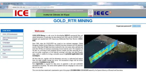
GOLD-RTR Mining is a web server for downloading GNSS-R experimental data and related information. In particular, the data collected from 2005 with the GOLD-RTR during the different experimental campaigns carried on by ICE-CSIC/IEEC, including GPS-SIDS at Greenland and Antarctica, whose analysis represents the fundamental core of the present thesis dissertation. Cardellach et al. (2011) provides several examples and tips about the processing possibilities of the whole dataset.

The GOLD-RTR Mining was developed at ICE-CSIC/IEEC as part of this PhD studies with the purpose of sharing the data acquired with the scientific community. The link address of the web server is:

❤tt♣✿✴✴✇✇✇✳✐❝❡✳❝s✐❝✳❡s✴r❡s❡❛r❝❤✴❣♦❧❞❴rtr❴♠✐♥✐♥❣

A screenshot of the index webpage is shown in Figure113.

After a free registration process, any identified user can access to the data records. These files are classified into WAV and INT, depending on the type of integration per-formed upon them. The category WAV refers to waveforms coherently integrated up to 1msec, thus containing phase information, whereas INT refers to power waveforms in-coherently integrated –typically– up to1sec. Note that WAV notation is then equivalent to the term RAW introduced in Chapter3(INT notation is consistent).

The files contain additional information, such as time-tag, PRN number or antenna’s polarization, following the structures described in Documentation → Formats from the

g

o

l

d

-r

t

r

m

in

in

g

:

a

w

e

b

s

e

r

v

e

r

o

f

g

n

s

s

-r

d

a

t

a

Figure113.: Screenshot of the GOLD-RTR Mining’s index webpage.

C

S E T U P

A software system was developed at ICE-CSIC/IEEC during the preparation of the GPS-SIDS experimental campaigns and as part of this PhD studies, with the purpose of re-motely operating the GNSS-R setup described in Chapter 3. Basically, it was required that an operator would be able to download acquired data, upload configuration files to the GOLD-RTR receiver and to monitor the whole system in real time and from a remote location. To do so, it was decided to build an architecture based on Apache Sub-version (SVN), a software Sub-versioning and revision control system distributed under an open source license (SVN, 2011), with several processes running in parallel in the local terminal unit (TU) and in a remotely located user end (UE) connected trough Internet or a local area network (LAN). The main characteristics achieved under this approach are:

• Robustness: Due to SVN transfer election, the system has implicit backups (SVN

repositories) and is robust against communication cuts.

• High data collection performance: GNSS-R data is collected at TU and then sent

to UE to be processed. If a communication cut happens, missing data at UE is again sent once communication is restored.

• Autonomy: Given that whole-campaign configurations can be predicted from a

single satellites’ orbit file, TU has a great autonomy. However, Internet/LAN con-nection is needed to monitor the data collection and to continuously update the configuration files with more recent orbits.

• Security: SVN configuration is password restricted. Direct access to TU via SSH/HTTP

connection is password and IP-address restricted.

Figure114provides a basic diagram of the software operation setup. Different colors identify those elements belonging to each subsystem, which are described next. The real time monitoring is made by means of a HTTP website located at UE to be accessed anywhere with an Internet connection. A screenshot example is shown in Figure115.

c

.

1

Software routine configure daemon at UE checks if there is a new igr-file (satellite rapid

software system for remote operation of a gnss-r setup

GOLD-RTR

gold_rtr Ethernet

scheduler daemon

�Observables Data

�_{Waveforms Data} �Integrated Waveforms

�Config Files

�Logs

OUTPUT FILES

500 GB 500 GB

subversion daemon

INTERNET / LAN

SVN inputs repository

configure daemon SVN COMMIT

IGSCB igr files

NEW

goldrtr_status receiver

SVN COMMIT SVN UPDATE

UDP

MySQL DB status

alerts

alerts

process �PDF Plots

�INTGEO Files (VisAD)

OUTPUT RESULTS

ping, ssh

TU

wavint

SVN outputs repository

SVN UPDATE

UE GPS SIDS WEB

Monitoring config file

Figure114.: System’s Architecture for remote operation of a GNSS-R setup. Different colors

identify those elements belonging to each subsystem: [blue]-Configuration, [green]-Control&Communications and [red]-Processing.

C.2 control&communications subsystem

then a long configuration autonomy in case of connection loss between UE and TU. User configuration (non-automatic) is also permitted by updating the SVN inputs repository. SVN offers a control of changes into the configuration files, allowing their tracking in an easy way.

c

.

2

The basic control of the collected data is done by means of the configuration files, which are automatically generated. The processscheduler daemonat TU continuously updates an

inputs-workspace, and make calls togold_rtrprocess depending on the different

configu-ration files. For each call, processgold_rtrcharges a new configuration in the GOLD-RTR,

and a new experiment begins. Given that this process should be working all the time, a

crontab is scheduled to periodically awake it. In addition, real time status flags are sent

bygold_rtrprocess every second with an UDP message to UE.

A SVN server at UE controls data storage and timing. Analerts process checks

Inter-net/LAN connection, data availability, etc., generating alert records and storing them in the MySQL database (DB). Similarly, processgoldrtr_statuschecks the status flags sent by gold_rtrand stores them also in the MySQL DB. In case of some incidence, the operator

at UE can then access to the remote TU via SSH and reactivate the system (if there is In-ternet/LAN connection). It is also possible to do a remote hardware reset of GOLD-RTR and TU via a web-based power supply. The router at TU is programmed to keep security by cutting intrusive SSH/HTTP connections.

c

.

3

At TU,gold_rtrgets the data from the GOLD-RTR via an Ethernet connection. For each

experiment, RAW data, INT data, log and configuration files are saved in a given folder structure called outputs, which is a work-copy of the SVN repository. Process subver-sion daemon continuously checks if output files are finished. Then, it compresses INT

files (bzip2) and commits the changes to the outputs SVN repository. RAW data is not transmitted due to a data transfer rate limitation (40GB/month).

At UE,process daemonchecks the changes into the outputs SVN repository, processing

s

o

f

t

w

a

r

e

s

y

s

t

e

m

f

o

r

r

e

m

o

t

e

o

p

e

r

a

t

io

n

o

f

a

g

n

s

s

-r

s

e

t

u

p

Figure115.: Screenshot of the Web-based monitoring system for GPS-SIDS.

D

d

.

1

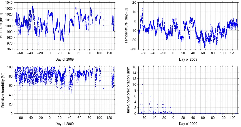
During the experimental campaign, meteorological records measured from a nearby ground Arctic Weather Station (53.516◦_{W, 69.253}◦_{N) were provided by DMI. The location} of this weather station is displayed in Figure 24. Time series of the observed pressure, temperature, relative humidity and precipitations are displayed in Figure 116. In addi-tion, a more relevant parameter for this study such as sea ice concentration was also provided. It was obtained by means of visual inspection and its evolution is shown in Figure117.

960 970 980 990 1000 1010 1020 1030 1040

Pressure [hPa]

−60 −40 −20 0 20 40 60 80 100 120

Day of 2009

−30 −20 −10 0 10 20

Temperature [deg−C]

−60 −40 −20 0 20 40 60 80 100 120

Day of 2009

0 20 40 60 80 100

Relative humidity [%]

−60 −40 −20 0 20 40 60 80 100 120

Day of 2009

0 2 4 6 8 10 12 14 16

Rain/Snow precipitation [mm]

−60 −40 −20 0 20 40 60 80 100 120

Day of 2009

Figure116.: Time series of the atmospheric pressure (top-left), temperature (top-right), relative

ancillary data from greenland’s campaign

0 20 40 60 80 100

Sea ice concentration (%)

20 40 60 80 100 120

Day of 2009

Figure117.: Sea ice concentration as visually estimated from Arctic Weather Station.

D.2 total zenith delay

d

.

2

The microwave signals on the two carriers L1 and L2 in the GHz band broadcasted by the GPS satellites are delayed by the ionosphere and the neutral atmosphere on their way to the ground receiver. The ionospheric refraction is dispersive and is usually cor-rected using both frequencies to obtain theionosphere-free linear combination, which

is a standard observable for geodetic applications. Moreover, it affects almost identi-cally both direct and reflected radio-links, thus canceling when subtracting both signals. The refraction in the neutral atmosphere is not dispersive and its value cannot be taken directly from dual-frequency measurements. It can only be derived by estimation tech-niques along with other parameters. Theneutralrefraction is mainly induced by dry air,

water vapor, clouds and rain, and is proportional to the masses of the specific compo-nents along the ray path. The delay is smallest in the direction of the zenith and increases approximately with the reciprocal of sine of the elevation angle ε. The elevation depen-dence is described by a mapping function. The total atmospheric delay ρtropoRx contained in a GPS observation at the receiver’s (Rx) position can be partitioned into two parts

(Niell,1996):

ρRxtropo =mhz(ε)·DhzRx+mwz(ε)·DwzRx (116) where Dhz is the zenith hydrostatic delay, Dwz the zenith wet delay, mhz the hydrostatic mapping function and mwz the wet mapping function. The total zenith delay (Dz) is the sum ofDhzandDwz. The delay in the dry air (the hydrostatic component) is proportional to the air masses and amounts to _∼2.5 m for measurements in the zenith. The delay from the water vapor has a much higher variability and it ranges from a few mm in arid regions to400mm in humid regions. The refractivity caused by water vapor’s permanent dipole is per mole about 17times that of dry air. Typically, the influence of clouds and rain are marginal, and cannot be computed from the GPS measurements. For extreme weather conditions their influence may reach10% in Dwz, normally it is smaller than5% (Solheim et al.,1999).

ancillary data from greenland’s campaign

Figure118.: Total Zenith Delay observed by GFZ’s geodetic receiver, together with the NWPM

values (ECMWF model). Plot provided by GFZ.

Figure119.: Wet component of the zenith atmospheric delay, observed by GFZ’s geodetic receiver.

Plot provided by GFZ.

D.3 polar ice charts

d

.

3

The Centre for Ocean and Ice at DMI regularly produces ice charts covering the Green-land Waters by combining in-situ with remote sensing measurements (PV-DMI, 2013). The ice charts are produced mainly to support navigation around Greenland, so their resolution is lower than the desired for the experimental site. Despite of that, all the available ice charts during the campaign were collected for the data analysis. An exam-ple is shown in Figure 120. The egg-codeof the different areas provides information on

three concepts: concentration, development stage (related to thickness), and form (floe size). The concentration is given in percentage, while the phase and form respond to a numeric code, detailed in Table24.

Figure120.: An example of ice chart provided by DMI from April3rd,2009. The approximated

monitorization area of the GNSS-R experiment is marked with a red square.

ancillary data from greenland’s campaign

CODE STAGE FORM

thickness floe size

0 ice free pancake ice

1 new ice small growlers

2 thin ice (<₁₀cm) growlers (<₂₀m)

3 young ice (10-30cm) small floe (20-100m) 4 10-15cm medium floe (100-500m)

5 15-30cm big floe (500-2000m)

6 winter ice (30-200cm) vast floe (2-10km)

7 30-70cm giant floe (>_10km)

8 30-50cm fast ice

9 50-70cm icebergs

Table24.: Sea ice egg-codes for development stage and form used in the DMI ice-charts that

might appear in the region of the experiment.

Figure121.: An example of sea-ice egg-chart transformed into a hexadecimal color code. From

up to bottom, code numbers (listed in Table24) for different characteristics of sea ice:

concentration (in %/10scale), development stage, and form.

D.3 polar ice charts

Figure122.: Edited egg-chart: rotated to align parallels with X-axis; cropped into a fixed ares (the

same for every plot); egg-chart information around the experiment site transformed into hexadecimal color (example from March27 2009).

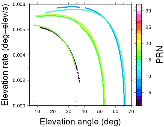
The ground tracks of the GNSS-R observations were then interpolated into the edited colored maps to extract the three concept values at each area of the track. For each PRN, it was then possible to generate three global campaign plots (one for each sea ice characteristic) to be then compared to other GNSS-R derived parameters. An example of global campaign plot is shown in Figure 123 (the way of how is made this type of representation is illustrated in Figure 67). The available ice-charts covered most of the campaign (after ice formation), with typical gaps of 3days. The values of one day were extrapolated up to three days forward, leaving blank the gap length beyond the third day.

0.09 0.12 0.15 0.18 0.21 0.24

sin(

ε

)

20 40 60 80 100 120

Day of Year 2009

0 10 20 30 40 50 60 70 80 90 100

Ice concentration [%]

Figure123.: Example of global campaign plot derived from a DMI’s ice chart: sea ice

concentra-tion interpolated to PRN02ground-tracks.

A particular case for this study is given when the egg-code indicatesfast icein the ice

ancillary data from greenland’s campaign

from land into sea. Unlike drift ice, it does not move with currents and wind. However it still moves with the tides, contributing then to the development of cracks and fissures in the ice cover and therefore, increasing the surface’s roughness, which is a key parameter for sea ice classification with GNSS-R employed in Belmonte et al. (2009).

D.4 ice surface temperature from modis

d

.

4

The ice surface temperature controls the rate of sea ice growth by means of the heat transfer at the ice-water interface (Tucker et al., 1992). This parameter is measured by the Moderate-Resolution Imaging Spectroradiometer (MODIS) (Hall et al.,2009) and can be obtained from NASA WIST server (nowReverb(NASA,2013)). The accuracy of these measurements is3.0K with4km resolution (Hall et al.,2004).

A set of samples were available at the experimental site during the campaign. The pixel’s location is shown at the top panel in Figure 124, whereas the time evolution of their average value is given on the bottom panel.

53.600˚W 53.500˚W 53.400˚W

69.200˚N 69.225˚N 69.250˚N 69.275˚N

0 5

km GNSS−R Receiver

250

255

260

265

270

IST [Kelvin]

20 30 40 50 60 70 80 90 100 110 120 130

Day of 2009

Figure124.: [Top] Position of MODIS’ data samples at the experimental site. [Bottom] Time series

ancillary data from greenland’s campaign

d

.

5

As explained in Chapter 2, accurate altimetry over Polar ocean scenarios may help to determine the free-board level of the ice sheets, which in turn is related to their thickness, a key parameter for sea ice characterization. A ground track from the Geoscience Laser Altimeter System (GLAS) from ICESat passes through the experimental area (top panel in Figure125). Unfortunately, only one coincidence in time for the whole campaigns’ period was available (96th day of year 2009), disabling the possibility of a proper statistical analysis. The time search was extended to 2005in order to increase the historic record and have a better idea about the range of altimetric measurements expected in the area.

The bottom panel in Figure 125 shows the results of the different GLA13 (Zwally et al.,2009) products found plotted with respect to latitude. These height measurements include tidal and atmospheric corrections and an additional software tool has been used for converting the reference ellipsoid from TOPEX/Poseidon to WGS84. Their single-shot error budget has a RSS (residual sum of squares) of 13.8 cm (Zwally et al., 2002). The data-sets and the software tools to work with them were obtained from NASA WIST server (now Reverb(NASA,2013)).

D.5 altimetric retrievals from glas

53.600˚W 53.500˚W 53.400˚W

69.200˚N 69.225˚N 69.250˚N 69.275˚N

0 5

km GNSS−R Receiver

22.0 22.5 23.0 23.5 24.0 24.5

Ellipsoidal height [m]

69.200 69.205 69.210 69.215 69.220 69.225 69.230 69.235

Latitude [deg]

19/03/2005

18/06/2005 23/03/2006

09/04/2007

31/10/2007

06/04/2009

Figure125.: [Top] Position of GLAS’ ground tracks at the experimental site. [Bottom] Height

re-trievals from ICESat GLAS at the campaign’s location for several days. The reference ellipsoid is WGS84in all cases. Tides effects are corrected. Note that only one track

ancillary data from greenland’s campaign

d

.

6

In order to retrieve information from the evolution of the sea ice cover from altimetric measurements, the variations of the surface level given by the ocean tide have to be corrected. In absence of in-situ tide gauges, the best option is to use a proper model. For this study, AOTIM-5 (Padman and Erofeeva, 2004) has been employed, a 5-km regular grid regional assimilation tide model of the entire Arctic Ocean. Figure 126shows the estimation made by the model during several days of the campaign at the experimental site. Notice that the variation with respect to the mean sea level is quite significant in this area, with daily differences up to2meters.

−1.0 −0.5 0.0 0.5 1.0

Distance from MSL [m]

1 2 3 4

Day of 2009

Figure126.: 3-day example of time evolution of the sea surface level estimated by AOTIM-5

model at the experimental site.

D.7 wind measurements from quikscat

d

.

7

ancillary data from greenland’s campaign

56.00˚W 55.00˚W 54.00˚W 53.00˚W 52.00˚W 51.00˚W

68.50˚N 68.75˚N 69.00˚N 69.25˚N 69.50˚N 69.75˚N

0 50

km

0 5 10 15 20

Wind speed [m/s]

−180 −120 −60 0 60 120 180

Azimuth [deg]

−65 −60 −55 −50 −45 −40 −35 −30 −25 −20 −15 −10 −5 0 5 10 15

Day of 2009

Figure127.: [Top] Position of QuikSCAT’s data samples closest to the experimental site. A land

mask of 50Km is applied. Time series of wind speed [center] and wind direction

[bottom] measurements from QuikSCAT.

D.8 palsar imagery

d

.

8

High resolution Radar imagery from satellite is especially useful for characterizing sea ice extensions. A few images from the Phased Array type L-band Synthetic Aperture Radar (PALSAR) onboard ALOS were provided by ESA (Rosenqvist et al., 2007). Fig-ure128shows the product with highest contrast, HH-pol backscattering coefficient (Hor-izontal polarization transmitted and received), for all the available days. The presence of thin sea ice is related to the lowest values of this coefficient (Wakabayashi and Sakai, 2011). Like in the case of GLAS, to have obtained more PALSAR images would have been an excellent opportunity for improving the analysis of our data-set, since this instrument works in the same frequency band than GPS and has a decent resolution for our experi-mental area (<_{100meters). At least, these pictures give a proof of the spatial variability} of the sea ice cover, showing that ice-water transitions might be expected along a 5 Km ground track.

−53.600˚ −53.500˚ −53.400˚

69.200˚ 69.225˚ 69.250˚ 69.275˚ 69.200˚ 69.225˚ 69.250˚ 69.275˚

−53.600˚ −53.500˚ −53.400˚

0 1000 2000 3000 4000 5000

PALSAR Amplitude HH−Pol

Figure128.: Polarimetric images from ALOS’ PALSAR taken at Disko Bay for different days

of the campaign: [Up-Left] December14th, 2008; [Up-Right] December19th, 2008;

[Down-Left] January 19th, 2009; [Down-Right] January 24th, 2009. The product

E

e

.

1

Atmospheric measurements were obtained from the official AWS (Automatic Weather Station) installed on Concordia base (PNRA, 2013). Air Temperature is represented in Figure 129. The situation is typical of the peak Austral summer, when the average air temperature value lies around -32◦C, showing a daily fluctuation of around12◦C with a minimum and a maximum of the period of -43◦C and -23◦C respectively.

Figure129.: Air Temperature (◦C) measured by the AWS at Concordia Station from1/12/2009

to15/01/2010. Plot provided by IFAC.

ancillary data from antarctica’s campaign

Figure130.: [Top] Wind speed (kt) and wind direction [bottom] measured by the AWS at

Con-cordia Station from1/12/2009to15/01/2010. Plots provided by IFAC.

E.2 snow temperature

e

.

2

These measurements started during DOMEX-1 experiment in 2005 and data were con-tinuously acquired until end of 2009. Due to the installation of a series of new nearby shelters during summer 2009, the probes that measure snow temperature in the first 10 meters were removed. For technical and scientific reasons, the shelter calledHelenenear

to the American tower was selected as new site (see location in Figure 27). The probes were then removed from their original location and a new10m hole was drilled (IFAC in cooperation with LGGE), causing a lack of data from December 2009to mid of January 2010.

The final setup consists of10 thermistors embedded in the snow at different depths down to 10m. The first 4probes were installed in a 1-meter pit at5,10, 50 and100cm deep. They are annually controlled and, due to the annual snow accumulation, reposi-tioned to the original depth. The other probes, with a depth interval between 200and 1000cm, were installed in a hole closed by a plastic cover. At the beginning of the experi-ment, the cover was placed1m deep. The snow accumulation is measured each year (i.e. the distance from snow surface to the cover) and the depth of the probes is then derived. Data acquired from 1/01/2010 to 30/01/2010 are represented in Figure 131. Snow temperature oscillated in the first 25 cm due to the forcing of daily air temperature variation and become stable at around1meter deep. The temperature profile was typical of the summer season showing maximum values near to the surface and decreasing with depth up to around 5 meters where reached the mean annual value of -55◦C. Similar values are expected for the days of the GNSS-R experiment.

Figure131.: Snow Temperatures measured at different depths at Concordia Station from

10/01/2010to30/01/2010. Note that it was after the GNSS-R campaign completed.

ancillary data from antarctica’s campaign

e

.

3

Contemporaneously to the tower observation experiment, other field activities were per-formed in order to characterize the ice-sheet properties in the first meters below the surface. This activity was conducted by IFAC in cooperation with scientists from LGGE, which have performed similar and complementary measurements in the snow pits. Up to 14 sites were analyzed and 25 snow pits digged from nearby locations: 20 down to 1m deep,4down to2m deep, and1at5m deep. In particular, a main5m pit was dug near the observation tower and stratigraphy of the snowpack was analyzed. In order to characterize the spatial variability of the ice-sheet structure, other snow pits (of around 1m depth) were digged in the direction NW-SE at12Km and 25 Km far from the base. The following parameters have been considered for each snow layer: shape and size of grains (Colbeck et al., 1990), temperature, hardness and density. Dielectric constant of snow was also measured each 10 cm using an electromagnetic probe called Snow Fork (Sihvola and Tiuri,1986).

The snow analysis included the identification of different snow layers, grain type (shape, size), density of different snow layers. Figure 132 presents an overview of the measured snow density at four different depths and different areas located around the Concordia station. As it can be seen, the higher percentage of measurement lie within the first meter, while few data were collected in the second meter or more.

Figure132.: Density of different snow pits executed in different areas around the Concordia base.

Plot provided by IFAC.

The deeper snow pit (5.3 meters) was executed near the American tower, and a syn-thesis is presented in Figure 133. The top panel shows the trend of the snow density every 50 cm. As it can be seen, some different densities can be observed in the first meters, while the density gradient is homogeneous at deeper layers. The bottom panel shows the comparison of snow density every10cm in two different times:2004and2009. Again, different layer densities can be observed in the first meters, while the profiles tend to be similar as the depth increases.

E.3 snow density

Figure133.: Mean snow density retrieved every 50 cm [top] and comparison with the results

ancillary data from antarctica’s campaign

In order to get a deeper profile of snow layers, these snow pit measurements were combined with data derived from ice cores (EPICA,2004), arriving down to700meters in the heart of Antarctica from Dome-C. The whole snow density profile is shown in

Figure 134. Overall, we can see that densities are very low at the surface layer, of the order of_∼0.3gr/cm3, presenting several sharp transitions of_±0.2gr/cm3during the first 10meters depth, to gradually increase up to a saturation value of0.92gr/cm3starting at

∼250m depth.

0.30 0.35 0.40 0.45 0.50 0.55

Snow density [gr/cm

3]

0 2 4 6 8 10

Snow depth [meter]

0.3 0.4 0.5 0.6 0.7 0.8 0.9 1.0

Snow density [gr/cm

3]

0 50 100 150 200 250 300 350

Snow depth [meter]

Figure134.: Snow density of the snow as a function of the depth, as provided by IFAC. [Top]

First10meters, [Bottom]350meters depth.

E.4 radiometric measurements from domex-2

e

.

4

With the objective of verifying the applicability of the East Antarctic plateau as an ex-tended target for calibrating and monitoring the performances of SMOS, DOMEX-2 ex-perimental campaigns were carried on in Dome-C in 2008-2009and 2009-2010by IFAC and other scientific partners. They mainly consisted in brightness temperature measure-ments in two polarizations (Vertical and Horizontal), taken by the L-band (1413 MHz) RaDomeX radiometer, for evaluating the long-time stability of L-band microwave emis-sion of the snow surface, while passive satellite data (from SMOS itself and AMSR-E in other frequency bands) were envisaged for evaluating the spatial stability.

ancillary data from antarctica’s campaign

Figure135.: [Top] Vertical (Tv) and Horizontal (Th) components of brightness temperature

mea-sured during three days of DOMEX-2experimental campaign (January13to16,2010).

Unexpected periodic fluctuations appear in Th. [Bottom] Position of the Sun

(Az-imuth and Zenith –elevation– in solid lines) compared with the radiometer’s antenna

orientation (dashed lines). The antenna has a3dB beamwidth of ∼30◦ (symmetric

for both E/H planes) in both polarizations. Notice that there is time coincidence between the crossing pass of the Sun into the antenna orientation and the fluctuation events. Plots provided by Giovanni Macelloni (IFAC).