Essays in applied economics

(1)

Essays in Applied Economics

Philipp Ager

TESI DOCTORAL UPF / ANY 2013

DIRECTOR DE LA TESI

Prof. Antonio Ciccone

(ICREA-UPF, Barcelona GSE and CREI)

(2)

(3)

(4)

(5)

Acknowledgements

I would like to thank my advisor Antonio Ciccone for his invaluable guidance and con-tinuous support while writing this thesis. I also owe much gratitude to Luigi Pascali for his helpful advice and insightful comments during my graduate studies. I am grateful to Fabrizio Spargoli for his co-authorship on the third essay of this thesis and to Markus Br¨uckner for his co-authorship on the fourth essay of this thesis. They are great col-leagues and I thank them for their patience and for sharing with me their knowledge on such important topics as on banking competition and cultural economics. Many other people at CREI and Universitat Pompeu Fabra have helped me during these years. A very incomplete list includes Gabrielle Fack, Albrecht Glitz, Giacomo Ponzetto, Marta Reynal-Querol and Joachim Voth. Their helpful comments and suggestions significantly improved the quality of my work. Special thanks also to Marta Araque and Laura Agust´ı at the GPEFM office for their superb administrative assistance.

Many thanks to my PhD colleagues and friends Stefan, Benedikt, Fabrizio, Silvio and Sofia for spending our time together at UPF and in Barcelona. My gratitude goes also to my friends from outside Barcelona: Manuel, Helmut and Claudia, Josef and Sibylle, Johannes, Siggi, Michael, Nils, Master, Boris, Steffen and Toni.

Finally, I am indebted to my parents, Wolfgang and Roswitha, and my grandmother Edith. Thank you for your continuous support, love and encouragement.

(6)

(7)

Abstract

This thesis consists of four essays. In the first essay, I examine how the historical planter elite of the Southern US affected economic development at the county level between 1840 and 1960. I find that counties with a relatively wealthier planter elite before the Civil War performed significantly worse in the post-war decades and even after World War II. In the second essay we investigate the link between religious membership and rainfall risk across US counties in the second half of the nineteenth century. Our results indicate that church membership and seating capacity were significantly larger in coun-ties likely to have been subject to greater rainfall risk. In the third essay, we examine the effect of removing restriction to bank entry on bank failures exploiting the introduction of free banking laws in US states during the 1837-1863 period. Our main finding is that counties in free banking states experienced significantly more bank failures. In the fourth essay we examine the effects that within-county changes in the cultural composi-tion of the US populacomposi-tion had on output growth during the age of mass migracomposi-tion. Our main finding is that increases in cultural fractionalization significantly increased output, while increases in cultural polarization significantly decreased output.

Resum

(8)

(9)

Forword

This thesis consists of four chapters. The first chapter examines how the historical planter elite of the Southern US affected economic development at the county level be-tween 1840 and 1960. To capture the planter elite’s potential to exercise de facto power, I construct a new dataset on the personal wealth of the richest Southern planters before the American Civil War. I find that counties with a relatively wealthier planter elite before the Civil War performed significantly worse in the post-war decades and even after World War II. I argue that this is the likely consequence of the planter elite’s lack of support for mass schooling. My results suggest that when during Reconstruction the US government abolished slavery and enfranchised the freedmen, the planter elite used their de facto power to maintain their influence over the political system and preserve a plantation economy based on low-skilled labor. In fact, I find that the planter elite was better able to sustain land prices and the production of plantation crops during Recon-struction in counties where they had more de facto power.

The second chapter examines the link between rainfall risk and religious membership in the late nineteenth-century US. Historically, religious organizations have often been at the core of local and cross-regional mutual assistance and social aid networks. Joining such networks can be more attractive in communities facing greater aggregate uncer-tainty as the value of partially insuring idiosyncratic shocks may increase with aggregate background risk. We show this in a theoretical model where aggregate background risk is driven by rainfall risk common to all members of the community. We then examine the link between religious membership – proxied by church membership or seatings – and rainfall risk across US counties in the second half of the nineteenth century. Con-sistent with our theoretical model the results indicate that religious membership was significantly larger in counties likely to have been subject to greater rainfall risk. This link is present among more agricultural counties and among counties with low popu-lation densities, but not among less agricultural or more densely populated counties. Among agricultural counties, a one-standard-deviation increase in rainfall risk is asso-ciated with an increase in church seating capacity of around 65 percent in 1860 and 32 percent in 1890.

(10)

was significantly higher in free banking states. We argue that the destabilizing effect of free banking is consistent with the view that bank competition leads to more risk taking. Our results suggest that the introduction of free banking led to more bank entry and a significant drop in the market share of incumbent banks.

(11)

Chapter 1 THE PERSISTENCE OF DE FACTO

POWER: ELITES AND ECONOMIC

DEVELOPMENT IN THE US

SOUTH, 1840-1960

1.1 Introduction

Wealth inequality may slow down economic growth (e.g. Galor and Zeira, 1993; Alesina and Rodrik, 1994; Deininger and Squire, 1998; Aghion et al., 1999). The historical plantation economies in the New World often serve as an extreme example. Although relatively rich in the past, these economies have fallen behind since. One explanation is that the great concentration of wealth in the hands of a small elite promoted the es-tablishment of oppressive institutions which were harmful for modern economic growth (Engerman and Sokoloff, 1997, 2002; Acemoglu et al., 2005; Acemoglu, 2008). Recent research has started to analyze whether historical wealth inequality might have been af-fecting economic development within the United States (Nunn, 2008; Galor et al., 2009; Ramcharan, 2010). I contribute to this literature by using county-level variation within the US South to examine how the relative wealth of the historical planter elite affected local economic development after the American Civil War and during the 20th century.1 Before the American Civil War, a large fraction of Southern wealth belonged to a small number of large plantation owners (Wright, 1970, 1978; Soltow, 1971, 1975). Historians have documented that their great wealth helped the planter elite to retain de facto power over economic institutions and politics after the Civil War, despite legal and political challenges like the abolition of slavery and black enfranchisement for example

1_{The US South had a more unequal wealth distribution in the nineteenth century compared to the}

(14)

(Wiener, 1976, 1978; Wright, 1986; Alston and Ferrie, 1999; Ransom and Sutch, 2001). I construct a new dataset on the personal wealth of the richest Southern planters before the Civil War (in 1860) to evaluate the long-run effects of the planter elite’s de facto power on local economic development. A key feature of my analysis is a measure of the planter elite’s relative wealth at the county level – which I regard as a proxy of their de facto power – based on these personal wealth data.2

My empirical analysis points to a significant negative association between the pre-Civil War wealth of the planter elite and levels of labor productivity across Southern counties in the post-war decades and even after World War II. Since my focus is on evaluating the long-run effects of the planter elite’s pre-Civil War wealth on local eco-nomic development rather than the ecoeco-nomic consequences of slavery per se, my em-pirical specifications always control for the extent to which local economies relied on slave labor before the Civil War.3 _{The negative association between the relative wealth} of the pre-Civil War planter elite and long-run labor productivity proves to be robust to a wide range of controls for geography and specialization in (certain types of) agriculture. My estimates imply that a two-standard-deviation increase in the relative wealth of the planter elite translates into productivity levels that are about 7 percent lower at the turn of the 19th century and 23 percent lower in 1950.

It is well understood that geography may have long-term effects on economic de-velopment (e.g. Diamond, 1997; Gallup et al., 1998; Rappaport and Sachs, 2003; Nunn and Puga, 2012). For example, climate and the types of available soils determine the agricultural production possibilities of an economy (e.g. Engerman and Sokoloff, 1997, 2002). I therefore examine whether the negative association between the relative wealth of the planter elite before the Civil War and long-run productivity levels in the US South is robust to a detailed set of controls for the geography, climate, and soil types of coun-ties. I find that controlling for geography does not affect my results. The economic development of counties in the US South may also have been determined by their his-torical specialization in agriculture, especially in producing large-scale plantation crops like cotton, tobacco, rice, and sugar. For example, high agricultural productivity may have led to high productivity in the past but low productivity in the 20th century as agri-culture crowded out manufacturing production and the learning externalities that might come with it (e.g. Matsuyama, 1992). I therefore reexamine the effect of the pre-Civil War planter elite’s relative wealth on economic development after controlling for the direct effect of specialization in (large-plantation) agriculture as well as a range of plan-tation crops. I continue to find a significant negative association between the relative wealth of the planter elite before the Civil War and long-run labor productivity, with a

2_{To my best knowledge, this is the first comprehensive dataset on the personal wealth of the Southern}

planter elite. Below I argue that the planter elite’s relative personal wealth reflects the elite’s de facto power better than existing measures of wealth inequality based on the farm size distribution.

3_{For evidence on the long-run effects of slavery within the US see, for example, Mitchener and}

(15)

quantitative effect that is similar to my baseline specifications.

The second contribution of this paper is to provide empirical evidence on specific mechanisms through which the planter elite’s use of de facto power may have affected Southern economic development after the Civil War. The empirical literature on the determinants of long-run economic growth has documented that underinvestment in hu-man capital is detrimental for economic development (e.g. Barro, 1991; Hanushek and Kimko, 2000; Castell´o and Dom´enech, 2002; Ciccone and Papaioannou, 2009; Becker et al., 2011). Also the theoretical literature on inequality and growth has argued that wealth inequality may delay economic development because of the elite’s reluctance to establish human capital promoting institutions (e.g. Galor and Moav, 2006; Galor et al., 2009). I therefore examine whether counties with a relatively wealthier planter elite before the Civil War accumulated less human capital following the Civil War and in the 20th century, controlling for the pre-Civil War illiteracy rate and the extent to which local economies relied on slave labor. My results indicate that illiteracy rates after the Civil War fell more slowly in counties with a relatively wealthier pre-Civil War planter elite. Moreover, I find that in 1940 and 1950 there was a significantly smaller fraction of high-school as well as college educated adults in counties with a wealthier planter elite before the Civil War. I also show that counties with a richer pre-Civil War planter elite were less likely to build so-called Rosenwald schools for black children.4 _Taken together, these results suggest that counties with a richer planter elite before the Civil War remained relative less productive well into the 20th century because of their low levels of human capital investment.

For the planter elite to be able to block reforms against their interests (such as mass education) they needed to maintain their political influence after the Civil War. While legal reforms like the abolition of slavery and black enfranchisement threatened the planter elite’s capacity to control Southern institutions, historians have documented that rich planters used their wealth to maintain economic and political influence (Shugg, 1937; Wiener, 1976; Ransom and Sutch, 2001). That is, planters were able to use the de facto power that came with their wealth to substitute for a loss of de jure power (Ace-moglu and Robinson, 2006, 2008a,b).5 One way in which the planter elite could have maintained their political influence after the Civil War was to support violent actions against black political representation. For example, Foner (1996, p. xxviii) reports that more than 10 percent of the black officeholders were victims of violence during the Reconstruction period (1865-1877). To investigate whether black officeholders were

4_{The Rosenwald Rural Schools Initiative (1914-1931) supported the construction of schools for black}

children in rural counties in the US South (Aaronson and Mazumder, 2011).

5_{Acemoglu and Robinson argue that the underlying distribution of political power in captured}

(16)

more likely to be victims of violence in counties where the planter elite was relatively wealthy before the Civil War, I combine my measure of the relative wealth of the planter elite with data from Foner’s directory of black officeholders during Reconstruction. My results indicate a positive and statistically significant association between the relative wealth of the pre-Civil War planter elite and violence against black officeholders fol-lowing the Civil War. This suggests that the planter elite may have used their de facto power to support violent actions against black officeholders.

Moreover, I show that the political influence of the planter elite persisted in the post-war period despite the legal and political reforms accompanying Northern intervention during Reconstruction.6 _{I find that 48 percent of the counties in Alabama and} Missis-sippi – two representative states of the so-called Deep South – had county delegates in their constitutional conventions at the beginning and towards the end or following the Reconstruction period with direct family connections to the pre-Civil War planter elite.7 I also show that family connections between the planter elite and county delegates in the constitutional conventions were more likely when the planter elite was wealthier. This suggests that – in line with Acemoglu and Robinson (2006, 2008a,b) – the planter elite used their de facto power to maintain their influence over the political system and preserve a planter-friendly regime.

One way to examine whether the greater de facto power of wealthier planters al-lowed them to better defend their interests when legal and political reforms during Re-construction brought losses to the elite’s de jure power is by studying the evolution of land prices during and following the Reconstruction period. Since land prices can be taken to capitalize agricultural profits (e.g. Plantinga et al., 2002; Deschˆenes and Green-stone, 2007), the planter elite’s capacity to defend their (agricultural) interests should show in land prices. I use a difference-in-difference approach to examine the cross-county association between the planter elite’s pre-Civil War wealth and land prices dur-ing Reconstruction and followdur-ing the adoption of the new constitutions, when planters managed to partly restore some of their de jure power. I find that during the Recon-struction period, land prices were relatively higher in counties with a wealthier planter elite. This suggests that the planter elite’s de facto power allowed them to capture local institutions for their own interest until the new constitutions restored some of their de

6_{So far there is little comprehensive data on the connections of the pre-Civil War planter elite to local}

politicians (delegates) after the Civil War. For anecdotal evidence on the political connections of planters after the Civil War see, for example, Moore (1978), Wynee (1986), Billings (1979), Foner and Mahoney (1995), and Cobb (1988).

7_{Both states had their first constitutional convention after the Civil War in 1865. With these}

(17)

jure power.8

My findings on higher land prices are consistent with the so-called paternalistic view of the planters’ behavior after the Civil War discussed in Alston and Ferrie (1993, 1999). According to this view, plantation owners offered blacks a set of amenities – such as protection from violence, improved housing, or medical care – in exchange of contractual arrangements that were favorable for plantation production. Alston and Ferrie argue that these paternalistic arrangements were easier to establish by wealthier planters because they required political influence. In line with the paternalistic view, my difference-in-difference analysis also yields that during Reconstruction, counties with a relatively wealthier pre-Civil War planter elite saw an increase in the production of plantation crops relative to all other main field crops grown in the US South (corn, wheat, barley, rye, oats, and sweet potatoes). I also show that there were significantly less lynchings and a higher share of black tenants in counties with a wealthier planter elite.

My work relates to the recent literature on economic inequality and development in the US. Galor et al. (2009) find a negative association between inequality in the farm size distribution and public spending on education at the county level at the beginning of the 20th century. Ramcharan (2010) documents that a more unequal farm size distribution at the county level leads to less redistribution between 1890 and 1930. Looking at the early 20th century, Rajan and Ramcharan (2011) show that counties with a more unequal farm size distribution had fewer banks per capita. On the other hand, Nunn (2008) does not find that a more unequal farm size distribution was detrimental for long-run economic development at the county level. One main difference between these contributions to the literature on the effects of wealth inequality on economic development and my work is that my measure of wealth inequality is based on personal wealth data rather than on data on farm size distributions. The two measures of wealth inequality can differ for two main reasons. First the data on farm sizes do not refer to ownership but to the farm as a unit of production. This is important as farms might have been operated by different tenants but owned by the same person. Farm tenancy was a feature of the US South even before the Civil War (Reid Jr., 1976; Winters, 1987; Bolton, 1994). For example, Bode and Ginter (2008) estimate tenancy rates from 3 to 40 percent for several counties in Georgia before the Civil War.9 _{Another reason why my measure of wealth inequality} differs from measures based on farm sizes is that my wealth measure also reflects the

8_{Once the planter elite largely regained their de jure political power, there were less needs to use de}

facto power to achieve their main objective: keeping the plantation system going (Wiener, 1976; Ransom and Sutch, 2001; Acemoglu and Robinson, 2008a). The restoration of de jure power should have benefited especially less wealthy planters who did not have the de facto power to sustain a planter-friendly system during the Reconstruction period.

9_{Since wealthy planters – the group of interest in this paper – often owned more than a single}

(18)

value of land. This is important if the planter elite tended to own the most valuable land. For my purposes it is therefore preferable to measure wealth inequality using personal wealth data.

Another difference between my work and the existing literature on the effects of wealth inequality in the US South is that my measure of wealth inequality is meant to proxy for the pre-Civil War planter elite’s capacity to defend their interests vis-`a-vis the rest of the society.10 _{Since I am particularly interested in the ability of the planter} elite to use their de facto power in order to repress the rest of the population, it seems sensible to measure wealth inequality by wealth of the planter elite relative to the total wealth in the county. Measures of wealth inequality based on the farm size distribution as used by Nunn (2008), Ramcharan (2010), and Rajan and Ramcharan (2011), seem better suited as a proxy of the distribution of de facto power among landowners.11 Us-ing the relative wealth of the planter elite as a measure of wealth inequality turns out to be key for my empirical findings. When I rerun the specification after replacing my measure of inequality with the Gini coefficients implied by the farm size distributions in each county, I do not find any statistically significant association between inequality and levels of economic development after the Civil War.

There is also a literature on the long-run effects of slavery on economic develop-ment in the US. Using variation across US states for the years 1880 to 1980, Mitchener and McLean (2003) find that the legacy of slavery adversely affects productivity. Nunn (2008) documents a negative link between slavery and current income per capita by ex-amining US state and county level data. Within the US South, Lagerl¨of (2005) finds that counties with a larger population share of slaves in 1850 are overall poorer today. However, more recently, Bertocchi and Dimico (2012) do not find any robust link be-tween slavery and current income per capita at the county level (but document an effect on current income inequality).12 _{Since my focus is on evaluating the long-run effects of} the planter elite’s pre-Civil War wealth on local economic development rather than the economic consequences of slavery per se, my empirical specifications always control for the extent to which local economies relied on slave labor.

The remainder of the paper is structured as follows. Section 2 provides a brief overview and discussion of the planter elite in the US South. Section 3 describes the data used in my empirical analysis. Section 4 analyzes the planter elite’s impact on the

10_{See Engerman and Sokoloff (1997, 2002), Acemoglu et al. (2005), and Acemoglu (2008) for work}

emphasizing the conflicts of interests between the elite and the masses and the elite’s capacity to repress others when it is in their interest.

11_{This becomes clear by considering an extreme example where all the land is distributed equally}

among a few land owners. Looking at the distribution of landholdings would yield to a complete equal distribution. On the other hand, the relative wealth of the farmer elite would depend on the (landless) population in the county, and could indicate great wealth inequality.

12_{On the economics of slavery in the US South see, for example, Fogel and Engerman (1974),}

(19)

post-war Southern economy. The last section concludes.

1.2 The Planter Elite in the US South

Historians have documented that a large fraction of wealth was in the hands of large plantation owners in the pre-Civil War South which resulted in a high degree of in-equality in the distribution of wealth (Wright, 1970, 2006; Soltow, 1971, 1975; Niemi Jr., 1977).13 _{The unequal distribution of wealth was a particularly salient feature of} the Southern agricultural sector before the Civil War.14 The reported average wealth of farmers owning slaves was $33,906 in 1860, about fourteen times larger than the wealth reported by farmers without slaves (see Ransom, 1989, Table 3.1, p. 63). Around 60 percent of the agricultural wealth was in the hand of the 10 percent richest Southern farmers and, even more strikingly, 24 percent of all wealth belonged to the 2 percent richest farmers (Ransom, 1989, p. 63). The great disparity of agricultural wealth points to the economic power of the richest farmers (planters) before the Civil War. Ownership of slaves accounts for a large part of this large disparity.15 Slave farms had an average personal estate of $19,828 compared to the $1,188 reported by free farms, and slave farms also had the better land (see Ransom, 1989, Table 3.1, p. 63). For example, in the Cotton South,16 the value of improved land of slave farms was $46.74 per acre in 1860 and about 3.5 times higher than the per acre value of improved farmland of farms without slaves (see Ransom, 1989, Table 3.2, p. 66).17 Since wealthy planters tended to own also the better land, it is important that my measure of wealth inequality accounts for the value and not the size of the planter’s real estate.

Before the Civil War it was the planter elite – who owned the large Southern

plan-13_{Soltow (1971, 1975) provides further information on the distribution of wealth in the United States}

during the 19th century. On race related economic inequality in the postbellum South see, for example, DeCanio (1979).

14_{For example, Acemoglu et al. (2008, Table 5.3) document that land inequality in the US South was}

considerably higher than in the northern US states in 1860.

15_{Slaves were a valuable asset during the antebellum period. The price for a prime field hand in}

historical dollars increased from approximately $600 around 1800 to $1,500 at the eve of the secession (Engerman et al., 2006). The value of a slave just before the Civil War was about $130,000 in 2009 dollars (see Williamson and Cain, 2011). Slave ownership was very concentrated and owning slaves in the South was the exception (Soltow, 1975, Table 5.3). According to the 1860 Census, there were 393,967 slaveholders out of 8.25 million free citizens that owned 3.95 million slaves in the South (Wahl, 2008, Tables 2 and 4) and the largest slaveowners held a disproportionate fraction of slaves within the slaveholder class. For example, in the Cotton South of 1860, large slaveowners with 50 or more slaves occupied one third of the total slave workforce (Wright, 1978, p. 31).

16_{Ransom (1989) refers to the states of Alabama, Georgia, Louisiana, Mississippi, South Carolina and}

Texas as Cotton South

17_{See also Wright (1970) on the agricultural wealth concentration in the Cotton South for the years}

(20)

tations and most of the slaves – that controlled Southern politics and institutions (Ran-som, 1989).18 _{With the adoption of the thirteenth amendment (in 1865), slavery and} involuntary servitude were outlawed. The ratification of the fourteenth amendment (in 1868) and the fifteenth amendment (in 1870) granted blacks citizenship and the right to vote.19 _{However, despite such major institutional changes, the existing planter elite} was able to sustain a plantation-based agricultural system after the Civil War. Economic historians have argued that the reason why the planter elite could maintain economic and political influence after the Civil War was their control over landholdings (Wiener, 1976; Ransom, 1989; Ransom and Sutch, 2001). It was one of the early purposes of the Freedmen’s Bureau to distribute land confiscated from former slaveowners to freedmen and finance the construction of black schools and emergency relief by selling the other confiscated property from former slaveowners (Ransom and Sutch, 2001, p. 82). A main setback for the Congress’ redistribution plans was the Amnesty Proclamation of May 1865, which restored all rights to property except as to slaves, and returned confis-cated land to their original owners (Ransom, 1989, p. 234).20 A bill proposing to grant 40 acres and $50 to every former slave who was head of a household was defeated by the Congress in 1867 (Ransom and Sutch, 2001, p. 82). As Wright (1986, p. 84) noted ”[...] the key to the survival of the plantation was the ability of the former slave owners to hold onto their land in the midst of intense legal and political struggles after 1865. In national politics, the planters successfully blocked proposals for land confiscation and redistribution to the freedmen.”

In addition to the political resistance against the redistribution of land, many South-ern whites were also reluctant to sell land to blacks (Ransom and Sutch, 2001, p. 87). Often the threat of violence against white sellers and prospective black purchasers in-creased the cost and risk of land sales, preventing black landownership (Ransom and

18_{The definition of the Southern planter elite varies in the economic history literature. Fogel and}

Engerman (1974) or Campbell (1982) define large planters by ownership of slaves for example. Fogel and Engerman define a large planter as slaveholder with at least 50 slaves. Campbell uses a less narrow classification defining large planters as owners of 20 or more slaves. Wiener (1976) defines the planter elite by landownership. According to Wiener, a planter needs to own at least $10,000 in real estate in 1850, $32,000 in 1860 and $10,000 in 1870 to be considered in the planter class.

19_{In general, the freedmen were now able to accumulate wealth and savings, acquire higher skills,}

start their own businesses (e.g. farming), and engage in politics (see e.g. Ransom and Sutch, 2001). The US Congress founded the Freedmen’s Bureau in 1865 to assist the freedmen in daily life. With the help of the Union Army and the Freedmen’s Bureau established the Republican administration some new institutions for blacks like a financial saving institution (the Freedman’s Saving and Trust Company) and school facilities. Moreover, black candidates were allowed to be elected as delegates for national and state governments and many served as public officeholders in local governments which brought political representation to the Afro-American community (Foner, 1988; Du Bois, 1999).

20_{The only exemption was made on the Sea Islands (a small stripe along the costs of Georgia and South}

(21)

Sutch, 2001, p. 87).21 _{That landownership remained extremely concentrated following} the Civil War is quite well documented. For example, see the evidence in Shugg (1937) based on Louisiana tax records, and in Wiener (1976) as well as in Ransom and Sutch (2001) based on the real estate holdings reported by the Census enumerators for coun-ties in Alabama.22 _{Moreover, there was not only a high degree of persistency in the} concentration of landownership, but also persistence in the planter elite’s identity. For five black belt counties in Alabama, Wiener (1978, p. 9) finds that 18 of the 25 planters with the largest landholdings in 1870 were in the group of the largest landholders in 1860 and 16 were in the group of the largest landholders in 1850.

Although the planter elite continued to own most of the Southern land, they lost direct control over the black workforce after the Civil War and it became a main chal-lenge for the planter elite to secure black labor (Alston and Kauffman, 2001; Ransom and Sutch, 2001; Naidu, 2010). Planters did not succeed in reintroducing the gang labor system on their plantations (Fogel and Engerman, 1974),23 _{they had turned to other} la-bor arrangements such as tenancy and sharecropping (Reid Jr., 1973; Shlomowitz, 1984; Ransom and Sutch, 2001).24 _{Southern states responded directly after the Civil War to} planters’ needs and introduced the so-called Black Codes – mainly vagrancy and anti-enticement laws – which intended to keep black labor immobile (Wilson, 1965; Cohen, 1976).25 _{The planter elite also used violent de facto power to keep black labor} work-ing on their fields. For example Wiener (1978, p. 62) writes that”Planters used Klan terror to keep blacks from leaving the plantation regions, to get them to work, and keep them at work, in the cotton field”, see also Trelease (1971) and Wiener (1979). Facing the potential threat of violence, freedmen often agreed to keep working on plantations in exchange for protection from Klan terror and other threats (Alston and Ferrie, 1985, 1993, 1999). Alston and Ferrie argue that planters with political influence protected the freedmen and also provided amenities such housing or medical care with the aim of

21_{Mississippi even enacted a law to prohibit black landownership after the Civil War. This law was}

however quickly overturned by the Freedmen’s Bureau (Ransom and Sutch, 2001, p. 87).

22_{Further studies with similar findings on the persistence of landownership are for example Huffman}

(1974) and Billings (1979).

23_{Engerman and Fogel argue that large-scale plantations employed slave labor in producing stable}

crops (rice, tobacco, sugarcane and cotton) during the antebellum period more efficiently by using a gang work system. The gang work system allowed slaveholder to allocate slaves efficiently among jobs. According to Fogel and Engerman (1977) gang work started to yield efficiency gains on plantations with 16 slaves or more. On the profitability of the Southern slavery economy see also David and Temin (1979), Wright (1979), and more recently Acemoglu and Wolitzky (2011).

24_{The efficiency of new labor arrangements such as sharecropping is discussed in Reid Jr. (1973),}

DeCanio (1974), Higgs (1977), and Ransom and Sutch (2001).

25_{Despite the Black Codes were repealed by the 14th amendment during Reconstruction, they were}

(22)

reducing monitoring costs and labor turnover.26 _{Since establishing such so-called} pater-nalistic arrangements was cheaper at larger scale and required political influence they were mostly used by wealthier planters.27

On the political side, the planter class primarily found its representation in the South-ern Democratic Party, which had the objective to restore the ”old SouthSouth-ern system” (Key, 1949; Foner, 1988; Stampp, 1965). When the Democratic party – the so-called Redeemers – gradually regained control over Southern politics in the late 1870s, they started to cut taxes and introduced labor and tenancy laws in favor of the landowners (Woodman, 1995; Foner, 1988). Most of the Southern states also reintroduced some of the former Black codes and imposed voting restrictions such as literacy tests and poll taxes, which restricted the political participation of blacks (Key, 1949; Kousser, 1974; Woodward, 1951).28

Acemoglu and Robinson (2006, 2008a,b) argue that the Southern elite’s exercise of de facto power after the Civil War explains why economic or policy outcomes in the US South were invariant to changes in de jure institutions.29 It required a series of ad-verse economic shocks – for example, the boll weevil infestation starting around 1890 (Lange et al., 2009), the Great Mississippi Flood in 1927 (Hornbeck and Naidu, 2012), the extension of the railroad system to the Deep South (Wright, 1986) and the demand for labor during wartime (Henri, 1975; Grossman, 1991) – combined with the

introduc-26_{With the rise of tenancy and sharecropping were many (black) farmers also often tied to their}

land-lords and local merchants by the way they had to finance their business (Ransom and Sutch, 1972, 2001). Local merchants – frequently with strong social ties to the planter class and in many cases the same per-son as the landlord – supplied credit to small farmers which were in general secured by crop liens. The credit conditions imposed by the merchants forced many of the tenants and sharecroppers into a from of debt peonage, see, for example, Ransom and Sutch (1972, 1975, 2001) and Wiener (1975).

27_{According to Alston and Ferrie (1985, 1993, 1999) emerged paternalistic arrangements as a response}

to the planter’s problem to secure a stable labor supply after the Civil War. It was in the interest of the planters to use their political influence to make paternalistic arrangements more valuable. Planters used their local political power (e.g. by influencing county courts and police) to ensure security for their black workforce. Outside the plantation created the planter elite a hostile legal environment (e.g. black disenfranchisement, low public spending for education, or anti-enticement laws) to impose external threats to black workers with the aim to impede their mobility.

28_{Feldman (2004) documents a drop of registered voters between 1900 and 1903 from 79,311 to just}

1,081 in fourteen Black Belt counties of Alabama. More recent studies are Chay and Munshi (2012), who analyze the link between political participation and black mobilization around the Reconstruction Era and Naidu (2012), who examines the political and economic effects of black disenfranchisement in the US South during the 19th century.

29_{More evidence on planters’ activities after the Civil War can be found, for example, in Alston and}

(23)

tion of immigration restrictions at the end of World War I to trigger black migration to the northern US states at a large scale30_{and a gradual decline of the planter elite’s} eco-nomic and political power (Alston and Ferrie, 1985, 1993, 1999).31 Still it took until the 1940s for the Southern states to escape the post-emancipation equilibrium and starting to converge towards the productivity levels of other US regions (Wright, 1986, 1999).

1.3 Data

My measure of the planter elite’s ability to exercise de facto power in a county is their relative personal wealth. To calculate the pre-Civil War planter elite’s relative personal wealth across counties, I use the US Census to compile an individual-level database on the personal wealth of members of the planter elite – defined as planters who owned at least 100 slaves – just before the American Civil War (1860).32 _{The US Census of 1860} reports personal data such as name, address, place of birth, value of real and personal estate and profession of each free person and, in a separate slave schedule, slaveholders are listed together with the slaves they own. This allows me to identify members of the planter elite and their personal wealth. According to the aggregated county statistics of the 1860 Census there are approximately 2,350 slaveholder in the planter elite as I de-fine it. My database contains individual-level information on about 85 percent of these slaveholders.33

To compile the individual-level dataset on large planters from the US Census files, I work with the genealogical websiteAncestry.com. This website provides digitized im-ages from all Census records before 1940 (including the slave schedules), and offers a search engine to locate the slaveholders by first, middle and last name, birthplace and year as well their place of residence. To identify the slaveholders with more than 100 slaves I counted the number of slaves owned by each slaveholder listed in the 1860 slave schedules. I then matched the names of the slaveholders in the slave schedule to the corresponding names reported in the schedule of free inhabitants. For some cases

30_{Before World War I, the Kansas Exodus of 1879 is the only known larger scale migration response of}

Afro-Americans to violence, bad labor conditions, and the loss of civil rights and political representation brought by the Redeemers in the US South (Painter, 1976). Estimates range between 15,000 to 60,000 black migrants (Van Deusen, 1936).

31_{For example Alston and Ferrie argue that the mechanization of the cotton harvest led to a decline of}

paternalistic arrangements in the US South.

32_{My definition of the planter elite intends to capture the most powerful and wealthiest pre-Civil War}

planters in the US South and is more narrow than the definitions used in the existing literature, see for example, Fogel and Engerman (1974), Wiener (1976), or Campbell (1982).

33_{I use a less restrictive definition when I could not identify a slaveholder in the Census of 1860. This is}

(24)

the search engine does not provide correct matches, because of the difficulty to decipher the handwriting of the enumerators. I then tried to match the slaveholders manually. Finally, I collected and entered the value of real and personal estate of each identified slaveholder in my database.

Table 1 reports the descriptive statistics of the members of the planter elite identi-fied in my dataset. In the 1860 Census, the average member of the planter elite was 50 years old, male, worked in the agricultural sector (about 90 percent listed as occu-pation planter or farmer) and reported on average $101,384 in real estate and $148,598 in personal estate. The average slaveholding was 154 slaves. With $248,320 of total wealth, the average member of the planter elite was 359 times wealthier than an aver-age free person in the US South in 1860 (the mean wealth is $692; the median wealth is zero).34 My descriptive statistics of the planter elite highlight that a small number of large plantation owners held a disproportionate fraction of wealth in the US South before the Civil War and resonate with the earlier findings of Wright (1970), Wright (1978), Soltow (1971), and Soltow (1975). The planter elite in my sample – 2006 in-dividuals who made up only 0.02 percent of the population of the US South – owned about 6 percent of the Southern wealth in 1860.

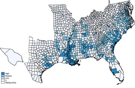
To obtain a measure of relative wealth of the planter elite at the county level, I aggre-gate the personal wealth of the planter elite in each county and divide it by total county wealth as reported in the aggregated county statistics of the US Census in 1860 (Figure 1 shows the spatial distribution of the relative wealth of the planter elite at the county level). Planters are assigned to their counties of residence in 1860. Hence, my measure of relative wealth of the planter elite can be expressed as

W ealthP E_c,₁₈₆₀ =

PP

p=1W ealthP Epc,1860

W ealthc,1860

!

. (1.1)

Summary statistics are reported in Appendix Table. The Data Appendix provides a detailed description of all other variables and data sources used in my empirical analysis.

1.4 The Planter Elite and the Southern Economy

I use the following baseline estimating equation to empirically investigate the link be-tween the relative wealth of the pre-Civil War planter elite and local economic develop-ment across Southern US counties,

ln(ycs) = α+λs+βW ealthP Ecs,1860+ ΓXcs,1860+ucs. (1.2)

34_{I retrieved the one percent random sample of the free population for the 1860 Census from the IPUMS}

(25)

The dependent variable, ln(ycs), stands for the ln total value added per worker which

is my measure of labor productivity at the county level. I include state fixed effects,

λ_s, to capture unobservable time-invariant state characteristics. The main right-hand side variable of interest is the fraction of 1860 wealth owned by the planter elite in countyc, W ealthP Ecs,1860, defined in (1). I also include a set of pre-Civil War county

characteristics,X_cs,₁₈₆₀, such as ln slaves, ln population, and ln area, to control for the extent to which local economies relied on slave labor and the county size.

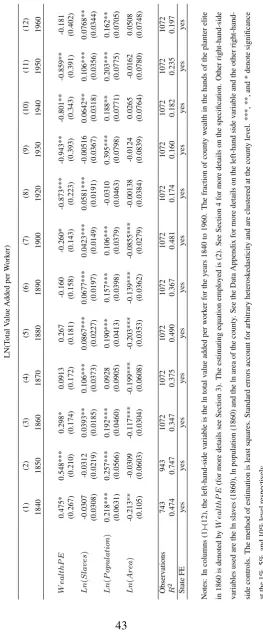
1.4.1 Direct Effect

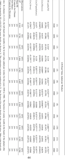
Table 2 presents my estimates of the link between the relative wealth of the pre-Civil War planter elite and levels of labor productivity looking at ten-year intervals between 1840 and 1960. The estimating equation is (2) and the method of estimation least squares. Columns (1)-(3) contain the estimates for the years before the Civil War. The estimates show a positive and statistically significant association between the relative wealth of the planter elite and total value added per worker between 1840 and 1860. In columns (4)-(12), I present the results for 1870 to 1960. The link between the relative wealth of the historical planter elite and total value added per worker remains positive in the immediate post-war decades 1870 and 1880, but is statistically insignificant. In 1890 there is a flip in the sign of the estimated coefficient on the relative wealth of the planter elite. Starting in 1900 and until 1950, I obtain a negative and statistically signif-icant link between the relative wealth of the historical planter elite and total value added per worker. The point estimate on the relative wealth of the planter elite in 1900 is sta-tistically significant with a p-value of 0.068.35 And for the period 1920 to 1950 the link between the relative wealth of the planter elite and total value added per worker is at least statistically significant at the 5 percent level. My estimates imply that a two-standard-deviation increase in the relative wealth of the planter elite translates into productivity levels that are about 4 percent lower at the turn of the 19th century and 14 percent lower in 1950. In 1960 the link between the relative wealth of the planter elite and total value added per worker is no longer statistically significant.

Researchers have pointed out that geographic factors affect long-run economic de-velopment (e.g. Diamond, 1997; Gallup et al., 1998; Rappaport and Sachs, 2003; Nunn and Puga, 2012). And Engerman and Sokoloff (1997, 2002) argue that climate and soils suitable for the production of plantation crops may have also fostered economic inequality.36 _{To address this issue, I add county-specific controls for geography to the} baseline estimating equation (2). The set of geographical controls includes mean eleva-tion, standard deviation in elevaeleva-tion, average yearly temperature, average yearly rainfall,

35_{I have no results for the year 1910, since there are no manufacturing data available from the 1910}

Census at the county level.

36_{For the relation between geography and economic inequality see, for example, Easterly (2007), Galor}

(26)

53 different soil types, growing degree days, cotton suitability as well the county’s lati-tude and longilati-tude.37 _{Table 3 reports the results on the association between the relative} wealth of the planter elite and levels of labor productivity after controlling for geog-raphy. Columns (1)-(3) present the results for the decades before the Civil War. The estimated coefficient on the relative wealth of the planter elite between 1840 and 1860 remains positive and statistically significant. In columns (4)-(12) I show the results on the link between the relative wealth of the planter elite and total value added per worker for the 1870-1960 period. The results are similar to Table 2, but quantitatively some-what stronger. As in the baseline specification the link between the relative wealth of the planter elite and total value added per worker is positive but statistically insignifi-cant in 1870 and 1880. The relationship between the relative wealth of the planter elite and total value added turns negative and statistically significant in 1890, and remains negative and statistically significant for the whole period until 1960. Between 1890 and 1950 the negative association between the relative wealth of the planter and total value added is statistically significant at the 1 percent level. In 1960 the negative associa-tion is statistically significant at the 5 percent level. The point estimates imply that a two-standard-deviation increase in the relative wealth of the planter elite translates into productivity levels that are about 7 percent lower at the turn of the 19th century and 27 percent lower in 1950.

To ensure that my results are not driven by the historical specialization in agriculture, and especially in producing large-scale plantation crops, I add a range of controls that are meant to capture differences in the extent of (large-plantation) agriculture across counties in the US South. These controls are the number of slaves working on large plantations, the fraction of land cultivated by large farms and the shares of Southern plantation crops (i.e. the shares of sugar, cotton, rice and tobacco production).38 _{Table 4} contains the results on the link between the relative wealth of the planter elite and levels of labor productivity after controlling for geography as well as the historical special-ization in large-plantation agriculture. Although the reported coefficient on the relative wealth of the planter elite for the pre-Civil War years remains positive, see columns (1)-(3), the effect is now only statistically significant in 1840. Columns (4)-(12) show the results on the link between the relative wealth of the planter elite and total value added per worker between 1870 and 1960. As in Table 3, there is a positive, but statistically insignificant, association between the relative wealth of the planter elite and total value added per worker in the immediate post-war decades 1870 and 1880. The relationship between the relative wealth of the planter elite and total value added turns negative and statistically significant in 1890. Between 1890 and 1950 the estimated coefficient on the relative wealth of the planter remains negative and at least statistically significant at the 5 percent level. In 1960 the link between the relative wealth of the planter elite and total

37_{I provide a detailed description of each geographic variable and its source in the Data Appendix.}

(27)

value added per worker becomes somewhat weaker and is only statistically significant with a p-value of 0.09. My estimates imply that after controlling for geography and his-torical specialization in large-plantation agriculture, a two-standard-deviation increase in the relative wealth of the planter elite translates into productivity levels that are about 7 percent lower at the turn of the 19th century and 23 percent lower in 1950.39

1.4.2 The Planter Elite’s Lack of Support for Mass Education

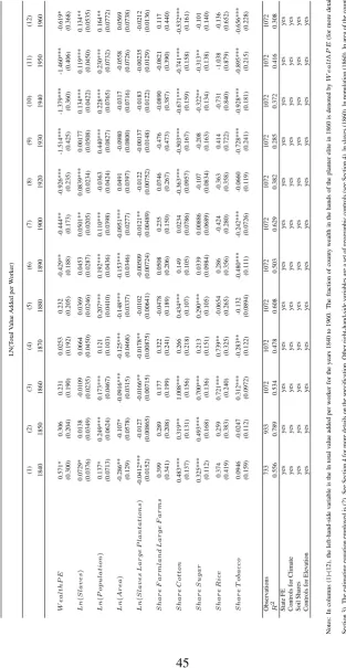
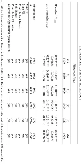
The literature on inequality and growth argues that an unequal distribution of wealth may be a hurdle for economic development because of the elite’s reluctance to establish human capital promoting institutions (e.g. Deininger and Squire, 1998; Galor and Moav, 2006; Easterly, 2007; Galor et al., 2009). Hence, I am interested in examining whether counties with a relatively wealthier planter elite before the Civil War had higher illiter-acy rates (conditional on pre-Civil War illiterilliter-acy rates) following the Civil War and at the beginning of the 20th century. Table 5 presents my estimates of the link between the relative wealth of the pre-Civil War planter elite and illiteracy rates after the Civil War between 1870 and 1930.40 _{The estimates are based on estimating equation (2). I use the} same set of control variables as in Table 4 and also account for the pre-Civil War illiter-acy rate in 1860. Between 1870 and 1930 there is a positive and statistically significant association between the relative wealth of the planter elite and illiteracy. Taken together my results indicate that illiteracy rates after the Civil War fell more slowly in counties with a relatively wealthier planter elite and may suggest that planters delayed the con-vergence of illiteracy rates in counties where they had more de facto power (wealth) before the Civil War.

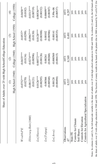
Table 6 contains the link between the relative wealth of the planter elite and the frac-tion of high-school as well as college educated adults in 1940 and 1950. The estimates are based on estimating equation (2) using the same set of control variables as in Table 5. Columns (1)-(2) of Table 6 show that there is a negative and statistically significant association between the relative wealth of the planter elite and the fraction of adults with high-school as well as college education in 1940. Columns (3)-(4) report the estimates for 1950. The link between the relative wealth of the planter elite and the fraction of high-school as well as college educated adults remains negative and statistically signif-icant.

Table 7 presents additional evidence indicating that the planter elite may have used

39_{As further robustness check I include the agricultural employment share and ln acres of farmland}

in 1860 as additional controls to account for the general historical specialization in agriculture of US Southern counties. The estimates are qualitatively similar to Table 4, but the link between the relative wealth of the planter elite and levels of labor productivity remains positive and statistically significant throughout all the pre-Civil War decades. The results are available upon request.

40_{The US Census reported information on literacy until 1930. Furthermore, there are no literacy data}

(28)

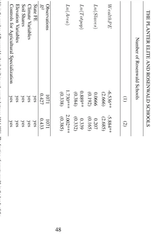
their de facto power to block educational improvements after the Civil War. The Rosen-wald Rural Schools Initiative supported the construction of schools for black children in rural areas between 1914 and 1931 to improve their educational attainment. The prin-ciple of the Rosenwald Fund was to provide help for communities where they received local support by local blacks, state, and county governments (Aaronson and Mazumder, 2011). One might therefore expect to have fewer Rosenwald schools built in counties were the planter elite had more de facto power to coordinate their resistance against black education. Columns (1)-(2) contain the estimates of the link between the relative wealth of the planter elite and the total number of Rosenwald schools built in the county between 1914 and 1931. The estimates are based again on estimating equation (2) us-ing the same set of control variables as in Table 5. The method of estimation is least squares. Column (1) shows that there is a negative and statistically significant associa-tion between the relative wealth of the planter elite and the total number of Rosenwald schools built. Since the Rosenwald Rural Schools Initiative intended to improve black education in rural areas, I also control for the pre-Civil War urban share in column (2). The estimated coefficient on the relative wealth of the planter elite remains negative and statistically significant at the 5 percent level. Hence, counties with a relatively wealth-ier planter elite before the Civil War were less likely to establish Rosenwald schools for black children. Taken together the results in Table 5-7 suggest that counties with a wealthier planter elite before the Civil War saw less human capital investment after the Civil War and during the first part of the 20th century. This could be a main reason why these counties remained relatively less productive well into the 20th century.

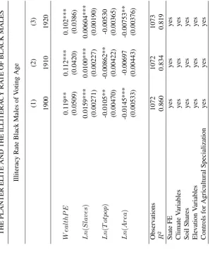
Moreover, the aggregated county statistics of the US Census provide information on the illiteracy of black adult men of voting age (age 21 and over) for 1900 to 1920, around the time when Southern states had introduced voting restrictions based on literacy tests and poll taxes (Key, 1949; Kousser, 1974; Naidu, 2012). In Table 8, I find that there is a positive and statistically significant association between the relative wealth of the planter elite and the fraction of illiterate black men of voting age between 1900 and 1920 using the same set of control variables as in Table 5. This again suggests that the planter elite may have used their de facto power to impede mass education. As an important by-product the planter elite’s lack of support of mass education may have also facilitated the exclusion of blacks from political participation. Since many of the planters’ political opponents were illiterate they could not interfere with the political goals of the planter elite once voting restrictions based on literacy tests were implemented.

1.4.3 The Planter Elite and the Use of de Facto Power

Violence against Black Officeholders

(29)

pol-itics and the economy. Foner (1996, p. xxviii) writes regarding black officeholders:

”Numerous Mississippi officials were threatened or driven from their homes during the 1875 campaign [...] Abram Colby, a member of Georgia’s legislature was beaten ”in the most cruel manner” by Klansmen in 1869. [...] Richard Burke, a minister and teacher in Sumter County, Alabama, who served in the state House of Representatives, was murdered in 1870. [...] In Edgefield County, South Carolina, violence was pervasive throughout Reconstruction.” Overall more than ten percent of the black officeholders were victims of violence during Reconstruction (Foner, 1996, p. xxviii).

Inspired by the anecdotal evidence I use Foner’s directory of Black Officeholders during Reconstructionto examine whether the use of violence against black officeholder was higher in counties with a wealthier planter elite before the Civil War. This direc-tory recorded over 1,500 black officeholders who served either at the national, state or local level. Foner (1996) also lists the names, county of residence and office positions of black officeholders who were victims of violence during their political career. I use this information to construct two measures of violence against black officeholders. The first measure is a binary variable which is unity if at least one black officeholder was a victim of violence in a county during Reconstruction. My second measure is the total number of black officeholders in a county who were victims of violence during Recon-struction.41 _{Column (1) of Table 9 shows the link between the relative wealth of the} planter elite and the probability that a black officeholder was a victim of violence using estimating equation (2). The estimated coefficient on the relative wealth of the pre-Civil War planter elite is positive and statistically significant at the 5 percent level. Column (2) reports estimates for the total number of black officeholders in a county who were victims of violence during Reconstruction. The estimated coefficient on the relative wealth of the pre-Civil War planter elite is again positive and statistically significant at the 5 percent level. These results suggest that the planter elite may have used their de facto power to support violent actions against black officeholders.

Political Connections

The journals of the constitutional conventions of several Southern states list the names of all participating delegates together with the counties (districts) they represented. With this information it is possible to evaluate whether the political influence of the planter elite at the county level persisted over time. For Alabama and Mississippi – two Deep South states with cotton-based economies – this information on the delegates can be found in theJournals of the Proceedings and Debates of the Constitutional Convention

of the states of Alabama (1865, 1875) and Mississippi (1865, 1890).42 This allows me

41_{Foner’s directory has no information on black officeholders for the states of Maryland, Missouri,}

Delaware and Kentucky.

42_{The journals of the proceedings and debates of the constitutional convention of the state of}

(30)

to investigate the delegates’ family connections to the pre-Civil War planter elite. I do this for the delegates that participated in the first constitutional convention after the Civil War as well as for delegates of the first constitutional convention after Reconstruction.

Both states held their first constitutional conventions after the Civil War in 1865. In these conventions the participating delegates introduced the Black Codes and planned the reestablishment of the ”old” Southern system. The Black Codes together with the constitutional conventions were suspended by the Reconstruction Acts in 1867 which placed ten former Confederate states under military control and required them to draft a new state constitution.43 Towards the end or following the Reconstruction period, Alabama held a constitutional convention in 1875 and Mississippi in 1890. These ventions were marked by the Democratic Party’s re-establishment of their political con-trol.44 I use three different selection criteria for the delegates’ connections to the pre-Civil War planter elite. First, if the delegate or a direct family member of the same household is listed in the slave schedule as slaveholder (Alternative 1). Second, if the total wealth of the delegate or a direct family member exceeds $10,000 in 1860 (Alter-native 2). The third criteria is a combination of the first two alter(Alter-natives and requires delegates or a direct family member to have at least $10,000 of wealth and being listed as slaveholder in 1860 (Alternative 3).45 I provide a detailed description of the data and how I linked the delegates to the pre-Civil War planter elite in the Data Appendix (pp. 31-36).

Table 10 contains the descriptive statistics for the constitutional conventions for Al-abama and Mississippi. In the constitutional convention of 1865, I find that 78 percent of Alabama’s delegates (or direct family members) and 69 percent of the delegates in Mississippi were listed as slaveowners in the slave schedules of the Census in 1860. The later constitutional conventions reveal a similar pattern. In Alabama, 73 percent of the delegates of the constitutional convention of 1875 had direct connections to slavehold-ers in 1860; in Mississippi, 60 percent of the delegates of the constitutional convention in 1890 had direct connections to slaveholders in 1860. Looking directly at whether the reported wealth of a delegate exceeds $10,000 in the 1860 Census yields similar results. If I use the selection criteria that requires delegates or a direct family member to have at least $10,000 of wealth and being listed as slaveholder in 1860, I obtain that 63 per-cent of the county delegates of the constitutional convention of Alabama in 1865 had a family connection to the pre-Civil War planter elite; for Mississippi, the corresponding

preference.

43_{Alabama and Mississippi introduced new constitutions in 1868. I do not consider the constitutional}

conventions in 1868, because delegates in both states were selected under military supervision.

44_{Foner (1996, Table 1) dates the end of Reconstruction in Alabama in 1874 and Mississippi in 1875.}

45_{If it was not possible to identify the delegate or a direct family member in the 1860 Census, but in}

(31)

number is 59 percent. In the 1875 constitutional convention in Alabama, 66 percent of the delegates had a family connection to the pre-Civil War planter elite; in the 1890 constitutional convention in Mississippi, 52 percent of the delegates had a family con-nection to the historical planter elite.

To examine the delegates’ connection to the pre-Civil War planter elite at the county level in Alabama and Mississippi, I construct a binary variable,P C_cs, for each county in Alabama and Mississippi that takes the value of unity if at least one delegate in both constitutional conventions had a family connection to the planter elite using the most stringent selection criteria (Alternative 3). This indicator variable should reflect the po-litical influence of the pre-Civl War planter elite in the constitutional conventions. I then investigate whether rich delegates with family connections to the planter elite were more likely in counties with a relatively wealthier planter elite using the following estimation equation

P Ccs =α+λs+βW ealthP Ecs,1860+γDelegatecs+ ΓXcs,1860 +ucs. (1.3)

The parametersλsare state fixed effects, and the variable of interest,W ealthP Ecs,1860,

is defined in (1). As controls I include the average number of county delegates,Delegate_cs, as well as the ln population and ln area, denoted by Xcs,1860, to control for the county

size. The method of estimation is probit.

In column (1) of Table 11, I show that there is a positive and statistically signif-icant association between the probability that a county is politically captured by the planter elite and the relative wealth of the planter elite.46 _{The estimated coefficient on} the relative wealth of the planter elite is statistically significant at the 1 percent level. In addition, I re-estimate equation (4) using a county panel specification

P Ccs,t =α+λs,t+βW ealthP Ecs,1860+γDelegatecs,t+ ΓXcs,1860+ucs,t. (1.4)

The dependent variable,P Ccs,t, is again a binary variable that is equal to unity in yeart

if at least one delegate in the county was listed as a slaveholder and reported more than $10,000 of wealth in the 1860 Census (Alternative 3). I replace the state fixed effects,

λs, by time varying state fixed effects,λs,t, which capture observable and unobservable

time varying characteristics at the state level.47

Column (2) of Table 11 reports the link between the relative wealth of the planter elite and the probability of having at least one county delegate with family connections

46_{I obtain qualitatively similar results when using Alternative 1 and Alternative 2 for the construction}

of the indicator variable, instead. These results are available upon request.

47_{The constitutional conventions after the Civil War in 1865 are coded as}_t_{= 1}_{and the constitutional}

(32)

to the planter elite using estimating equation (5). The estimated coefficient on the rel-ative wealth of the planter elite is positive and statistically significant at the 5 percent level. Since some counties were allowed to send more than one delegate to the con-stitutional conventions, I also examine the link between the number of rich delegates with family connections to the pre-Civil War planter elite and the relative wealth of the planter elite before the Civil War. Column (3) reports the least squares results us-ing the same right-hand-side controls as in column (2). The estimated coefficient on the planter elite’s relative wealth is positive and statistically significant at the 1 percent level. Hence, there is a positive and statistically significant association between the rel-ative wealth of the pre-Civil War planter elite and the number of delegates sent to the constitutional conventions that had family connections to planter elite. In line with Ace-moglu and Robinson (2006, 2008a,b), my findings suggest that the planter elite used their de facto power to capture local politics in order to preserve a planter-friendly po-litical system in the post-Civil War South.

Land Prices

The planter elite’s ability to exercise de facto power should have allowed them to better defend their interests during the Reconstruction period when they had less de jure power. Since historians have documented that planters maintained land ownership after the Civil War (e.g. Shugg, 1937; Wiener, 1976; Ransom and Sutch, 2001), a main objective of the planter elite should have been to preserve their rents from land. As land prices can be taken to capitalize agricultural profits (e.g. Plantinga et al., 2002; Deschˆenes and Greenstone, 2007), the planter elite’s capacity to defend their (agricultural) interests should show in land prices. To explore whether wealthier planters were better able to defend their interests in times with less de jure power, I therefore compare the evolution of land prices at the county level during Reconstruction, when legal reforms like the abolition of slavery or the enfranchisement of freemen for example brought losses in the elite’s de jure power, with the period when Southern states overrode the Reconstruction conventions and planters recouped de jure power. My estimating equation is

ln(LPcs,t) =λc+λs,t+βT Es,t×W ealthP Ecs,1860+ucs,t. (1.5)

The dependent variable, ln(LPcs,t), stands for the ln value of farmland per acre in

countycof state s in year t. I also include county fixed effects,λc, and time varying

state fixed effects, λs,t, to capture time-varying state characteristics. T Es,t is a binary

variable that takes the value one for all years after the Civil Warand before the state overrode its Reconstruction convention (the direct effect of the treatment effect,T Es,t,

is captured by the time-varying state fixed effects).48 The main variable of interest,

(33)

T Es,t×W ealthP Ecs,1860, denotes the interaction of the treatment effect and the

rela-tive wealth of the planter elite. If the planter elite was better able to sustain land prices during Reconstruction in counties where they had more de facto power, the estimated coefficient on the interaction term should be positive.

Panel A of Table 12 contains my results on the link between land prices and the planter elite’s wealth during Reconstruction and following the adoption of the new con-stitutions for the decades 1870 to 1930. The method of estimation is least squares. Col-umn (1) shows that during Reconstruction land prices were relatively higher in counties where the planter elite had more de facto power. The estimated coefficient on the in-teraction term is statistically significant at the 1 percent level. Columns (2)-(3) report the results when I also interact the treatment effect with other pre-Civil War county characteristics, like the reliance on slave labor and county size in column (2) and vari-ables capturing the historical specialization in plantation agriculture in column (3). The estimated coefficient on the relative wealth of the planter elite remains statistically sig-nificant at the 1 percent level in both cases.

I also estimate a version of equation (6) that focuses on the sample of contiguous counties that lie on the opposite sides of state borders. The advantage of comparing only contiguous border counties is their similarity, which mitigates the concerns related to the heterogeneity between treatment and control group. To implement this so-called border county approach I need to modify estimating equation (6) by including additional time varying border segment fixed effects. These border segment controls account for common observable and unobservable factors that vary across state border segments over time. The new estimation equation is

ln(LPbcs,t) =λc+λb,t+λs,t+βT Es,t×W ealthP Ecs,1860+ubcs,t (1.6)

where the main difference to estimation equation (6) is the inclusion of time varying border segment fixed effectsλ_b,tand restricting the sample to border counties.49 Figure 2 highlights the border counties used in my empirical analysis.50

Panel B of Table 12 shows the estimates for the border county approach for 1870 to 1930. The method of estimation is least squares.51 The results reported in column

Reconstruction convention. A list of the timing of the first constitutional conventions after Reconstruction of each Southern State is available from the author upon request.

49_{The border county approach follows closely the regression discontinuity design of Black (1999),}

Dube et al. (2010), Fack and Grenet (2010), and Naidu (2012) for example.

50_{Note that a border county can be in multiple border segments.}

51_{To account for within-state over time and within border segment over time correlations I use a}

Essays in applied economics