Essays on Monetary and Fiscal Policy

Texto completo

(1)Essays on Monetary and Fiscal Policy. Ma. Beatriz de Blas Pérez June 2002.

(2) Universitat Autònoma de Barcelona Departament d’Economia i d’Història Econòmica International Doctorate in Economic Analysis. Essays on Monetary and Fiscal Policy PhD Dissertation presented by Ma. Beatriz de Blas Pérez. Supervisor: Dr. Hugo Rodríguez Mendizábal. Barcelona, June 2002. i.

(3) A mi familia. ii.

(4) Barcelona, June 2002. Acknowledgements. This work is highly indebted to my supervisor Hugo Rodríguez. Thank you Hugo for your support, patience and advice. Di¤erent parts of this work have also bene…ted from many comments of Jordi Caballé, Jim Costain, and Andrés Erosa who have seen and contributed to the evolution of this dissertation. Thanks also to the International Doctorate in Economic Analysis, and the Departament d’Economia i d’Història Econòmica of the Universitat Autònoma de Barcelona for these 5 years. I would also like to acknowledge GREMAQ and the Economics Department at Université de Toulouse I, in particular Patrick Fève and Franck Portier for their hospitality and help on this work. Also thanks to Larry Christiano, Fabrice Collard, Jürgen von Hagen, Belén Jerez, Jordan Rappaport, Federico Ravenna, Carl Walsh, and other participants in the workshops and conferences in which the articles of this dissertation have been presented. I do not want to …nish without giving special thanks to José García Solanes and Arielle Beyaert who introduced me into research in Economics and motivated me to begin this PhD program. To conclude, I want to acknowledge my friends both at the IDEA programme and in Murcia for still being there after this time. Also to my family, who have su¤ered the ups and downs in these doctoral years and have encouraged me to continue and improve in my work. Finally, thank you Jim, for everything. iii.

(5) Contents List of Figures. vi. List of Tables. vii. Introduction viii Bibliography . . . . . . . . . . . . . . . . . . . . . . . . . . . . . . . . . . . . . . . . . xvi. I. Monetary Policy. 1. 1 Interest Rate Rules Performance under Credit Market Imperfections 1.1 Introduction . . . . . . . . . . . . . . . . . . . . . . . . . . . . . . . . . . . 1.2 Related literature . . . . . . . . . . . . . . . . . . . . . . . . . . . . . . . . 1.3 The model . . . . . . . . . . . . . . . . . . . . . . . . . . . . . . . . . . . . 1.3.1 Households . . . . . . . . . . . . . . . . . . . . . . . . . . . . . . . 1.3.2 Firms . . . . . . . . . . . . . . . . . . . . . . . . . . . . . . . . . . 1.3.3 Financial intermediaries . . . . . . . . . . . . . . . . . . . . . . . . 1.3.4 Entrepreneurs . . . . . . . . . . . . . . . . . . . . . . . . . . . . . . 1.3.5 The monetary authority . . . . . . . . . . . . . . . . . . . . . . . . 1.4 Equilibrium . . . . . . . . . . . . . . . . . . . . . . . . . . . . . . . . . . . 1.5 Solution method . . . . . . . . . . . . . . . . . . . . . . . . . . . . . . . . 1.6 Parameter values . . . . . . . . . . . . . . . . . . . . . . . . . . . . . . . . 1.7 Quantitative properties of the models . . . . . . . . . . . . . . . . . . . . 1.8 Dynamic properties of the models . . . . . . . . . . . . . . . . . . . . . . . 1.8.1 E¤ects of credit market imperfections . . . . . . . . . . . . . . . . 1.8.2 Dynamics under the Taylor rule . . . . . . . . . . . . . . . . . . . . A shock to technology . . . . . . . . . . . . . . . . . . . . . . . . . A shock to money demand . . . . . . . . . . . . . . . . . . . . . . 1.9 Conclusions and further research . . . . . . . . . . . . . . . . . . . . . . . Appendix: Equilibrium conditions . . . . . . . . . . . . . . . . . . . . . . . . . Bibliography . . . . . . . . . . . . . . . . . . . . . . . . . . . . . . . . . . . . . Tables . . . . . . . . . . . . . . . . . . . . . . . . . . . . . . . . . . . . . . . . . Figures . . . . . . . . . . . . . . . . . . . . . . . . . . . . . . . . . . . . . . . .. iv. . . . . . . . . . . . . . . . . . . . . . .. . . . . . . . . . . . . . . . . . . . . . .. . . . . . . . . . . . . . . . . . . . . . .. . . . . . . . . . . . . . . . . . . . . . .. 2 2 5 8 10 13 15 16 19 20 23 23 26 28 28 30 30 33 35 37 39 43 46.

(6) 2 Can Financial Frictions Help Explain the Performance of 2.1 Introduction . . . . . . . . . . . . . . . . . . . . . . . . . . . 2.2 Data and sample selection . . . . . . . . . . . . . . . . . . . 2.3 A monetary economy . . . . . . . . . . . . . . . . . . . . . . 2.3.1 Households . . . . . . . . . . . . . . . . . . . . . . . 2.3.2 Firms . . . . . . . . . . . . . . . . . . . . . . . . . . 2.3.3 Financial intermediaries . . . . . . . . . . . . . . . . 2.3.4 Entrepreneurs . . . . . . . . . . . . . . . . . . . . . . 2.3.5 Monetary policy . . . . . . . . . . . . . . . . . . . . 2.4 Equilibrium . . . . . . . . . . . . . . . . . . . . . . . . . . . 2.5 Parameters of the model . . . . . . . . . . . . . . . . . . . . 2.6 Calibration results . . . . . . . . . . . . . . . . . . . . . . . 2.6.1 Discussion . . . . . . . . . . . . . . . . . . . . . . . . 2.6.2 Interest rate rules, monitoring costs, and shocks . . 2.7 Conclusions . . . . . . . . . . . . . . . . . . . . . . . . . . . Bibliography . . . . . . . . . . . . . . . . . . . . . . . . . . . . . Tables . . . . . . . . . . . . . . . . . . . . . . . . . . . . . . . . . Figures . . . . . . . . . . . . . . . . . . . . . . . . . . . . . . . .. II. the US Fed? . . . . . . . . . . . . . . . . . . . . . . . . . . . . . . . . . . . . . . . . . . . . . . . . . . . . . . . . . . . . . . . . . . . . . . . . . . . . . . . . . . . . . . . . . . . . . . . . . . . . . . . . . . . . . . . . . . . . . . . . . . . . . . . . . . . . . . . . . . . . . . . . . . . . . . . . .. . . . . . . . . . . . . . . . . .. . . . . . . . . . . . . . . . . .. . . . . . . . . . . . . . . . . .. Fiscal Policy. 54 54 57 60 60 63 65 66 68 69 72 73 78 81 82 85 88 94. 95. 3 Debt Limits and Endogenous Growth 3.1 Introduction . . . . . . . . . . . . . . . . . . . . . . . . . . . . . . . 3.2 The model . . . . . . . . . . . . . . . . . . . . . . . . . . . . . . . . 3.2.1 Households . . . . . . . . . . . . . . . . . . . . . . . . . . . 3.2.2 Firms and technology . . . . . . . . . . . . . . . . . . . . . 3.2.3 Government . . . . . . . . . . . . . . . . . . . . . . . . . . . The debt limit . . . . . . . . . . . . . . . . . . . . . . . . . 3.3 Competitive equilibrium . . . . . . . . . . . . . . . . . . . . . . . . 3.4 Balanced growth path . . . . . . . . . . . . . . . . . . . . . . . . . 3.5 Parameter values . . . . . . . . . . . . . . . . . . . . . . . . . . . . 3.6 Long run e¤ects of …scal policy . . . . . . . . . . . . . . . . . . . . 3.6.1 An increase in the labor tax rate (¿ w ) . . . . . . . . . . . . 3.6.2 A reduction in the government spending to output ratio (³) 3.7 Transitional dynamics . . . . . . . . . . . . . . . . . . . . . . . . . 3.7.1 An increase in the labor tax rate (¿ w ) . . . . . . . . . . . . 3.7.2 A reduction in the government spending to output ratio (³) 3.8 Welfare analysis . . . . . . . . . . . . . . . . . . . . . . . . . . . . . 3.9 Conclusions and extensions . . . . . . . . . . . . . . . . . . . . . . Appendix: First order conditions for the competitive equilibrium . . . . Bibliography . . . . . . . . . . . . . . . . . . . . . . . . . . . . . . . . . Tables . . . . . . . . . . . . . . . . . . . . . . . . . . . . . . . . . . . . . Figures . . . . . . . . . . . . . . . . . . . . . . . . . . . . . . . . . . . .. v. . . . . . . . . . . . . . . . . . . . . .. . . . . . . . . . . . . . . . . . . . . .. . . . . . . . . . . . . . . . . . . . . .. . . . . . . . . . . . . . . . . . . . . .. . . . . . . . . . . . . . . . . . . . . .. . . . . . . . . . . . . . . . . . . . . .. . . . . . . . . . . . . . . . . . . . . .. . . . . . . . . . . . . . . . . . . . . .. 96 96 100 100 103 104 105 107 109 111 112 113 115 116 117 119 120 122 125 127 129 131.

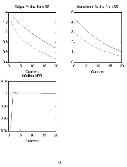
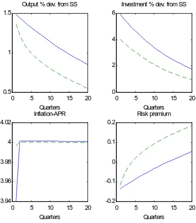
(7) List of Figures 1.1 1.2 1.3 1.4 1.5 1.6 1.7 1.8 2.1. Real US GDP versus the spread between the Bank Prime rate and the Six-month Treasury-bill rate. . . . . . . . . . . . . . . . . . . . . . . . . . . . . . . . . . . . Impulse response functions to a technology shock under the constant money growth rule. . . . . . . . . . . . . . . . . . . . . . . . . . . . . . . . . . . . . . . . Impulse response functions to a technology shock in the Symmetric information case. . . . . . . . . . . . . . . . . . . . . . . . . . . . . . . . . . . . . . . . . . . . Impulse response functions to a technology shock in the Asymmetric information case. . . . . . . . . . . . . . . . . . . . . . . . . . . . . . . . . . . . . . . . . . . . Di¤erences in impulse response functions to a technology shock. . . . . . . . . . . Impulse response functions to a money demand shock in the Symmetric information case. . . . . . . . . . . . . . . . . . . . . . . . . . . . . . . . . . . . . . . . . Impulse response functions to a money demand shock in the Asymmetric information case. . . . . . . . . . . . . . . . . . . . . . . . . . . . . . . . . . . . . . . . Di¤erences in impulse response functions to a money demand shock. . . . . . . . The evolution of output, in‡ation, federal funds rate and a measure of risk premium in the US during 1959:4-2000:3. . . . . . . . . . . . . . . . . . . . . . . . .. 3.1 3.2 3.3 3.4 3.5 3.6. 46 47 48 49 50 51 52 53. 94. Changes in the GPF model for di¤erent taxes on labor income. . . . . . . . . . . 131 Changes in the GUF model for di¤erent taxes on labor income (¿ w ). . . . . . . . 132 Changes in the GPF and GUF models for di¤erent tax rates on labor income (¿ w ).133 Changes in the GPF model for di¤erent government spending to output ratio (³). 134 Changes in the GUF model for di¤erent government spending to output ratio (³). 135 Changes in the GPF and GUF models for di¤erent government spending to output ratio (³). . . . . . . . . . . . . . . . . . . . . . . . . . . . . . . . . . . . . . . . . . 136 3.7 The dynamics of the GPF model after a rise in the labor tax rate (¿ w ). . . . . . 137 3.8 The dynamics of the GPF model after a fall in the government spending to output ratio (³). . . . . . . . . . . . . . . . . . . . . . . . . . . . . . . . . . . . . . . . . 138. vi.

(8) List of Tables Table 1.1: Parameter values. . . . . . . . . . . . . . . . . . . . . . . . . . . . . . . . . Table 1.2: Nonstochastic steady state values. . . . . . . . . . . . . . . . . . . . . . . . Table 1.3: Summary statistics. . . . . . . . . . . . . . . . . . . . . . . . . . . . . . . .. 43 44 45. Table Table Table Table Table Table Table. 88 88 89 90 91 92 93. 2.1a: Instability tests. . . . . . . . . . . . . . . . . 2.1b: Instability tests (continued). . . . . . . . . . 2.2: Estimated moments (Data). . . . . . . . . . . 2.3: Estimated moments (Pre- and Post-Volcker). 2.4: Estimated moments (¹c = 0). . . . . . . . . . 2.5: Estimated moments (¹c = 0:4727). . . . . . . 2.6: Estimated moments. . . . . . . . . . . . . . .. . . . . . . .. . . . . . . .. . . . . . . .. . . . . . . .. . . . . . . .. . . . . . . .. . . . . . . .. . . . . . . .. . . . . . . .. . . . . . . .. . . . . . . .. . . . . . . .. . . . . . . .. . . . . . . .. . . . . . . .. . . . . . . .. . . . . . . .. Table 3.1: Parameter values. . . . . . . . . . . . . . . . . . . . . . . . . . . . . . . . . 129 Table 3.2: Balanced growth path values. . . . . . . . . . . . . . . . . . . . . . . . . . . 129 Table 3.3: Welfare e¤ects of …scal policies. . . . . . . . . . . . . . . . . . . . . . . . . . 130. vii.

(9) Introduction This dissertation focuses on the analysis of monetary and …scal policy issues in macroeconomies with …nancial market imperfections.. Macroeconomic research is based on models that aggregate the decisions of many rational agents interacting in a completely speci…ed environment. Keeping track of these interactions is di¢cult, so most in‡uential macroeconomic models are based on strong simplifying assumptions. More recently, mainly due to the advance in computational methods, some of these unrealistic assumptions can be relaxed, opening the door to much deeper analysis of the mechanisms that move the economy. This dissertation’s study of imperfect …nancial markets is one example of the recent trend to greater realism in macroeconomics. The now widespread use of dynamic stochastic general equilibrium models for the analysis of the macroeconomy has been one of the main steps forward. As the name suggests, these models are …rst dynamic, capturing the intertemporal character of economic decisions. Second, they allow for some degree of uncertainty by assuming the stochastic evolution of certain variables that a¤ect the agents’ decisions. And …nally, the analysis is developed in a general equilibrium framework. This means that …rst the individual behavior of each agent in the economy is modeled based on microeconomic foundations, and then put together with the behavior of other agents in viii.

(10) a logically coherent way. All these elements, that constitute the core of modern macroeconomic analysis, are employed in this thesis. In addition, some of the traditional assumptions are relaxed, mainly the fact that …nancial markets are perfect. When imperfect credit markets are considered, the role of macroeconomic policy is ampli…ed, because imperfections introduce new mechanisms for the transmission of the policy decisions.. This dissertation is composed of three chapters and is structured in two parts. The …rst part is focused on monetary policy issues, and consists of two chapters. Chapter 1 deals with the e¤ects of monetary policy in an economy with credit market imperfections where the central bank’s monetary policy instrument is the interest rate. Chapter 2 analyzes the role of these credit market imperfections in the reduction of output and in‡ation volatility experienced in the US since the 1980s. The second part is devoted to the analysis of …scal policy issues. Chapter 3 studies the e¤ects on growth and welfare of imposing limits to the issue of public debt.. The …rst part of this thesis studies the performance of monetary policy rules in economies with and without credit market imperfections. Theoretical attempts to explain the way economic conditions in‡uence policy makers’ decisions, and how these choices are transmitted to the rest of the economy have been developed mainly under the assumption of perfect credit markets. However, there is little doubt that credit markets are far from perfect. In any contractual relationship involving a future outcome, like the one between borrowers and lenders, there is one part of the contract (usually borrowers) with more information about his own performance than the other (lenders). This private information enjoyed by borrowers is often re‡ected in the interest rate characterizing the contract. Transparent, well-known …rms will obtain funds from ix.

(11) very diversi…ed sources. However, small, new …rms will …nd it more di¢cult to raise funds and may often depend on a unique source of …nance. According to recent empirical work (Bernanke, Gertler and Gilchrist [2], and Gertler and Gilchrist [5]), the existence of …nancial frictions such as these may amplify and propagate the movements in output. If this is the case, analyzing the e¤ects of central banks’ decisions abstracting from …nancial frictions might be misleading, in particular if central bankers are concerned with macroeconomic stabilization issues, and use interest rates as instruments to conduct monetary policy. In Chapter 1, the e¤ects of endogenously driven monetary policy versus an exogenous constant money growth rule are investigated in a limited participation framework. Following the empirical literature (e.g. Clarida, Galí and Gertler [3]), I will assume that the central bank conducts monetary policy through an interest rate rule and is concerned with both in‡ation and output stabilization. The imperfections arise due to asymmetric information emerging in the production of capital, which introduces a kind of …nancial accelerator in the economy. The main results of this chapter can be summarized as follows. I obtain that the model economy …ts US data reasonably well. In particular, the setup with credit market imperfections is able to account for some stylized facts of the business cycle absent in the standard frictionless case. This makes it a good candidate to analyze the e¤ects of monetary policy. Regarding the stabilization of shocks, the use of interest rate rules in a limited participation setup has the opposite e¤ects compared with new Keynesian models. More concretely, in a limited participation model, the use of interest rate rules helps stabilize both output and in‡ation in the face of technology shocks, whereas there is a trade-o¤ between stabilizing output or in‡ation if the shock is to money demand. Finally, the e¤ects of a Taylor rule are stronger –either more strongly stabilizing or more strongly destabilizing, depending on the type of shock– when there. x.

(12) are …nancial frictions in the economy. This research can be extended in three complementary ways. One direction is the calibration of the coe¢cients of the rule under credit market imperfections. This could provide a better representation of real data in order to investigate the e¤ects of di¤erent monetary policy rules. Another line of research would lead to the derivation of the optimal monetary policy rule in a scenario of …nancial frictions. Rotemberg and Woodford [8] develop this topic in a sticky price model without …nancial frictions. They conclude in favor of backward-looking rules whenever private agents are forward-looking. It seems interesting to test the robustness of Rotemberg and Woodford’s results in a limited participation setup allowing for …nancial frictions. Finally, given the importance of variables such as the risk premium, which a¤ect the cost of borrowing, on the implications of …nancial frictions, research could also focus on how monetary policy performance would change if some indicator of the credit market imperfections is included in the rule. Possible candidates for this purpose are, for example, the bankruptcy rate and the risk premium.. Chapter 2 analyzes whether frictions in credit market or changes in the shock processes may have contributed to the reduction in macroeconomic volatility observed in the US since the 1980s. This reduced volatility has been mostly attributed to the way monetary policy has been conducted before and after Paul Volcker being the Chairman of the US Federal Reserve. In particular, most empirical research identi…es two di¤erent policy rules for the Pre- and PostVolcker eras (e.g. Clarida, Galí and Gertler [4], and Judd and Rudebusch [6]). These estimated rules re‡ect a central bank less concerned with output and in‡ation stabilization in the PreVolcker than in the Post-Volcker period. The focus of this chapter di¤ers from previous literature in the fact that …nancial frictions are considered when estimating the reaction function of the central bank. Doing this is important xi.

(13) for three reasons. First, because of the evidence presented in the …rst chapter, and elsewhere in the literature, about the ampli…cation and propagation e¤ects of shocks induced by the existence of …nancial frictions. Second, because the e¤ects of monetary policy can also be altered by the presence of these frictions. And third, because due to the development of …nancial markets, the degree of …nancial frictions themselves may have changed. There are several conclusions worth pointing out from this chapter. First, the analysis of the US data from 1959:4 to 2000:3, including a measure of risk premium, indicates a structural break at 1981:2. This point, close to the usual 1979:3, can be explained by two events. First, the existence of some lags in the implementation of monetary policy after Paul Volcker. But secondly, this breakpoint is obtained once a series of risk premium is considered. This may re‡ect other policy measures such as the implementation of the Economic Recovery Tax Act in March 1981 that implied a general reduction in corporate and individual income-tax rates a¤ecting the …nancing resources of …rms. Once a breakpoint has been identi…ed, the limited participation model with credit market imperfections that was developed in Chapter 1 is used to calibrate an interest rate rule for each subsample. In this framework, I also analyze whether other factors, such as …nancial frictions or changes in the shock processes, may have contributed to the stabilization of the economy, together with the monetary policy rule followed by the central bank. In the absence of …nancial frictions, the results con…rm the widely recognized change in the conduct of monetary policy by reporting substantially di¤erent interest rate rules before and after 1981:2. However, in contrast with the empirical literature, the calibration fails to assign more weight to in‡ation stabilization in the second subsample. This failure is resolved when a positive level of monitoring costs is introduced. Interestingly, in this case the procedure yields two calibrated rules that are much. xii.

(14) closer to each other than those found in the absence of frictions. That is, there is not such a big change in the monetary policy rule once monitoring costs are included. This may suggest a key role for credit market imperfections in the stabilization of monetary policy. When the rule, monitoring costs, and shocks are allowed to change across time, the calibration reports two interest rate rules re‡ecting a central bank more concerned with stabilizing in‡ation than output after 1981:2. The degree of …nancial frictions is reduced by 10% after 1981:2. Regarding shocks, money demand processes vary between samples, whereas technology innovations remain relatively stable across time, which is consistent with standard literature. Although doubtless there are other ways to improve the realism of this model of the US Fed, the analysis developed in this chapter is one step forward towards the understanding of the behavior of central banks and their e¤ects on the whole economy. After this, the next step would be a welfare analysis of the performance of the US Fed, that is, how far the rules identi…ed by the calibration in this chapter are from the optimal ones.. The second part of the dissertation turns to …scal policy issues and investigates the consequences on growth and welfare when the government …nancial options are restricted by the imposition of a limit to debt issue. The e¤ects of public debt in growth models has usually been analyzed by imposing no limit on the behavior of debt except a no-Ponzi game condition. Little attention has been paid to tighter constraints on public borrowing. This is the focus of Chapter 3. This topic has gained growing interest in the last years, mainly because of the criteria imposed on EMU countries by the Maastricht Treaty and later reinforced by the Stability Pact. These criteria led many countries to undertake strong …scal policy measures in order to reduce de…cits and debt. The existing literature analyzing limits on public debt is not very large. Moreover, growth issues are not the focus in most of those papers. On the other hand, research on growth xiii.

(15) has not explored debt ceiling issues. The study undertaken in this chapter tries to …ll in the gap by analyzing the e¤ects on growth and welfare of imposing limits to government debt. In Chapter 3, the model economy displays endogenous growth and allows government spending to have two di¤erent roles, either as a productive input (as in Barro [1]) or as services in the utility function, in which case it is private capital that drives growth (as in Romer [7]). Government spending can be …nanced through taxes on labor and issuing debt. In this framework, I study the efects of di¤erent …scal policies (changes in labor tax rates and the ratio of government spending to output) with and without debt limits in the balanced growth path. In the long run, if there is no debt limit, the growth e¤ects of raising labor income taxes are negative, regardless of the role of government spending. However, which role public spending plays in the economy is crucial for the growth e¤ects of changes in the ratio of public expenditures to output. In the presence of a limit to debt, higher labor tax rates have a positive e¤ect on growth if government spending is productive. However, when private capital drives growth, raising taxes on labor only serves to reduce the incentives to work, with a negative e¤ect on the growth rate. I also investigate the dynamic e¤ects of imposing a more restrictive …scal policy in order to attain a debt limit with a lower debt to output ratio, compared with an economy without limits which stays at its balanced growth path. This analysis is done for the case in which government spending is a productive input. I …nd that raising taxes to lower debt leads the economy to a new balanced growth path with higher growth and lower taxes, because of the productive role of government spending in this model. By the same reason, a …scal policy consisting of reducing government spending over output has the opposite e¤ects, reducing growth and output. Regarding welfare, raising labor income taxes imply a lower welfare cost of reducing debt than does cutting government spending.. xiv.

(16) A useful extension to this research would be to set up the second best problem. The idea is to allow the government to optimally design …scal policy taking into account …rst order conditions from individuals’ optimization. Here, the Ramsey problem may allow the government to choose just the optimal tax structure, taking as given government spending or deciding on both …scal variables. Additionally, new insights will be drawn from the introduction of debt limits into the government’s decision.. xv.

(17) Bibliography [1] Barro, R. J. (1990). “Government Spending in a Simple Model of Endogenous Growth.” Journal of Political Economy, 98, no. 5, part 2: S103-125. [2] Bernanke, B., Gertler, M. and Gilchrist, S. (1996). “The Financial Accelerator and the Flight to Quality.” Review of Economics and Statistics, 78, no. 1 (February): 1-15. [3] Clarida, R., Galí, J., and Gertler, M. (1998). “Monetary Policy Rules in Practice. Some International Evidence.” European Economic Review, 42: 1033-1067. [4] Clarida, R., Galí, J., and Gertler, M. (1999). “Monetary Policy Rules and Macroeconomic Stability: Evidence and Some Theory.” Quarterly Journal of Economics, 115: 147-180. [5] Gertler, M., and Gilchrist, S. (1995). “The Role of Credit Market Imperfections in the Monetary Transmission Mechanism: Arguments and Evidence.” Scandinavian Journal of Economics, 95, no. 1: 43-64. [6] Judd, J. P., and Rudebusch, G. D. (1998). “Taylor’s Rule and the Fed: 1970-1997.” Federal Reserve Bank of San Francisco Economic Review 3: 3-16. [7] Romer, P. M. (1986). “Increasing Returns and Long-run Growth.” Journal of Political Economy, 94, no. 5: 1002-1037. [8] Rotemberg, J. J., and Woodford, M. (1999). “Interest-rate Rules in an Estimated Sticky Price Model.” In Monetary Policy Rules, ed. John B. Taylor: NBER Business Cycles Series, vol. 31: 57-119.. xvi.

(18) Part I. Monetary Policy. 1.

(19) Chapter 1. Interest Rate Rules Performance under Credit Market Imperfections 1.1. Introduction. How do interest rate rules perform under credit market imperfections? Do they have the same stabilization properties in such an environment as compared with the frictionless case? Theoretical attempts to explain the way economic conditions in‡uence policy makers’ decisions, and how these choices are transmitted to the rest of the economy have been developed mainly under the assumption of perfect credit markets. However, there is little doubt that credit markets are far from perfect. In any contractual relationship involving a future outcome, like the one between borrowers and lenders, there is one part of the contract (usually borrowers) with more information about his own performance than the other (lenders). This private information enjoyed by borrowers is often re‡ected in the interest rate characterizing the contract. Transparent, well-known …rms. 2.

(20) will obtain funds from very diversi…ed sources. However, small, new …rms will …nd it more di¢cult to raise funds and may usually depend on a unique source of …nance. Gertler and Gilchrist [19], and [20] provide evidence that this is the case for US manufacturing …rms. How and when can these imperfections be observed? In the face of uncertainty about a future repayment on their loans, lenders will charge higher interest rates to the riskier borrowers. Figure 1.1 con…rms this intuition. It reports the evolution of the spread between the Bank Prime rate and the Six-month Treasury-bill rate for the period 1970:1-2000:2, as well as the real GNP for the same period.1 There are two things worth pointing out here. First, during the whole period, the average spread is positive (250 basis points), implying a risk premium paid by …rms issuing this type of bonds. Second, the chart clearly shows the countercyclical character of this spread with respect to GNP, with a correlation of -0.15 for the whole sample.2 This suggests that in good times, when GNP is high, the …nancial imperfections diminish. The opposite is true in a recession. According to some empirical analysis (for example, Bernanke, Gertler and Gilchrist [3]) the presence of such time-varying imperfections may help amplify the movements in output. If this is the case, analyzing the performance of monetary policy rules abstracting from credit frictions might be misleading, in particular if central bankers are concerned with macroeconomic stabilization issues. In this paper I investigate the performance of monetary policy governed by interest rate rules in economies with and without credit market imperfections. Money will have real e¤ects 1. The …gure shows a reduction in the variability of both series around 1984:1. McConnell and Pérez-Quirós. [26] document this change in US output as a structural break, mainly driven by durable goods. Although not analyzed by these authors, in this …gure it is observed that the risk premium mimics this change experienced by output. 2. This correlation is -0.17 for the sample period 1970:1-1983:4, and -0.33 for the sample period 1984:1-2000:2.. 3.

(21) in the model, because I assume limited participation of households in …nancial markets. Credit market frictions are introduced through asymmetric information in the production of capital. The way monetary policy rules behave in such a framework is analyzed by studying the e¤ects of shocks to technology and money demand. Empirical work shows that most central bankers appear to be following interest rate rules in the conduct of monetary policy (Clarida, Galí, and Gertler [11]); therefore it seems appropriate to focus on interest rate rules, as opposed to money growth rules, in studying the e¤ects of monetary policy. However, in order to get more insight into the mechanisms at work, I will compare two policy rules: an exogenous constant money growth rule, and a traditional Taylor rule. The main contribution of this paper is threefold. First, several features of monetary models (mainly, interest rate rules and credit market imperfections) are introduced together in a limited participation setup to get a framework in which monetary policy issues can be easily addressed. Second, the model’s capability to account for some stylized facts in business cycles dynamics is quantitatively analyzed. And third, focusing on Taylor type rules, this framework is used to analyze the stabilization properties of monetary policy. The main results of the paper can be summarized as follows. The model with …nancial frictions turns out to be a useful scenario to analyze some stylized facts in business cycle dynamics absent in standard monetary models. Some of these facts are the negative correlation between output growth and risk premium, the e¤ects of capital prices on output, and the high volatility of investment observed in the data. It turns out that in a limited participation setup the use of interest rate rules to conduct monetary policy has the opposite stabilization e¤ects when compared with a sticky price setting. Finally, it is observed that a Taylor rule has stronger e¤ects, either stabilizing or destabilizing, when there are credit market imperfections in the. 4.

(22) economy. This con…rms the hypothesis that monetary policy may be a¤ected by the presence of credit market imperfections. The innovations of this analysis in relation with the existing literature on credit market imperfections and monetary policy issues is analyzed in detail in the next section. Section 1.3 develops the model, introducing the role and features of each agent in this economy. Section 1.4 de…nes the equilibrium. In sections 1.5 and 1.6, the solution method, and parameter values employed are speci…ed, respectively. Section 1.7 quanti…es the properties of the model and compares them with real data. The model dynamics are analyzed in Section 1.8. Finally, Section 1.9 closes the paper.. 1.2. Related literature. This work is closely related to three other papers that investigate the e¤ects of …nancial frictions in the business cycle. The papers that originally motivated this analysis are by Fuerst [15] and Gertler [18]. The third one is the work by Bernanke, Gertler and Gilchrist [4]. Fuerst addressed the question of whether the presence of …nancial frictions distort the impulse and propagation of technology and monetary shocks. His model economy is also a limited participation setup in which imperfections in credit markets arise in the production of capital goods. Unlike the current study emphasis on interest rate rules, the framework chosen by Fuerst is such that the monetary authority employs money supply as the policy instrument. However, Fuerst’s analysis di¤ers in some key points. First, he does not …nd signi…cant di¤erences in the dynamics of the model after allowing for …nancial frictions. Therefore, in his model …nancial frictions do not have much role for impulse and propagation. Second, his model is not able to replicate the negative correlation between output and risk premium observed in the data. 5.

(23) In a comment to Fuerst’s paper, Gertler [18] highlights the crucial role of the elasticity of net worth with respect to output in this type of analysis. The argument goes as follows. According to the data, net worth (for example, entrepreneurs’ pro…ts) shows a high elasticity with respect to output growth. In times of high output, net worth will be high too. This will reduce the need for external …nancing and at the same time, will diminish the cost of external funds. This helps replicate the negative correlation between output and risk premia observed in the data. I internalize this fact in my analysis. In contrast to the two papers above, I consider a central bank concerned on both output and in‡ation stabilization, and with the nominal interest rate as its instrument. With these ingredients I analyze how credit market imperfections may alter the monetary transmission mechanism. The following is obtained. First, I …nd amplifying and persistent e¤ects of credit market imperfections because net worth responds strongly to output. This ampli…cation is visible in spite of the stabilizing e¤ects of the rule. I go on to do a quantitative assessment of the interaction between output, investment, labor, and the risk premium, which were not spelled out in Gertler’s suggestions. As I show below, this economy implies that technology shocks are stabilized, and money demand shocks destabilize prices with slightly output stabilization, in clear contrast with new Keynesian models of the business cycle. New Keynesian models predict that the use of interest rate rules would stabilize the economy in the event of shocks to money demand. This follows from the assumption of some nominal rigidity (in prices, wages or both), which makes output be demand-determined. In such a setting, any distortion arising from the demand side (and therefore a¤ecting output) can be neutralized by changing the money supply (that is, using the interest rate as an instrument). Why does the opposite occur in this paper? Here, with the. 6.

(24) limited participation setup, output becomes supply-determined and aggregate demand is left the role of determining the price level. Thus shocks a¤ecting aggregate supply can be neutralized by monetary policy if the interest rate is the instrument, whereas the opposite is true when money demand shocks are considered. This is because unlike new Keynesian models, in a limited participation setup changes in money supply will a¤ect both …rms and households decisions, inducing movements in both the aggregate supply and aggregate demand curves. Finally, this paper shows that the rule appears to have stronger e¤ects (either stabilizing or destabilizing) in the presence of credit market imperfections. As will be explained in Section 1.8, the supply side e¤ects of shocks in this model are emphasized in the presence of …nancial frictions. This is because of the upward sloped supply of investment goods. In this case, the …rms’ borrowing needs are hit by the additional e¤ect of the higher cost of capital a¤ecting their labor and investment decisions. Furthermore, changes in the interest rate also have an e¤ect on such decisions, like an in‡ation tax on investment. In a similar vein, Bernanke, Gertler and Gilchrist [4] analyze the role of credit imperfections arising in the demand for capital in a sticky price model. Although their setup di¤ers from mine in many ways, there are several common points. Their analysis focuses on the ampli…cation and propagation issues of …nancial frictions (what they call the …nancial accelerator ). In their model the central bank also follows an interest rate rule, reacting only to lagged in‡ation and interest rate, without any weight on output stabilization. Unlike here, in their paper they do not consider stabilization issues of monetary policy. This is important because as my analysis makes clear the way monetary policy is implemented may o¤set the amplifying e¤ects of …nancial frictions just by including some output stabilization into the objectives of the monetary authority. Summing up, in this paper it is shown that a model that …ts relatively well data is able to. 7.

(25) account for the e¤ects of …nancial frictions and yet tell us something about the transmission of monetary policy when the interest rate is the instrument. Indeed, the interest rate rule becomes more e¤ective in the presence of credit market imperfections, if the economy is a¤ected by a technology shock, and induces more variability on prices and output when the economy is a¤ected by money demand shocks.. 1.3. The model. The model economy is a cash-in-advance environment with two additional frictions. The …rst one allows for the non-neutral e¤ects of money by assuming limited participation of households in …nancial markets. The second one introduces credit market imperfections in the production of capital. Households in this economy supply labor to …rms and obtain wage payments in return. In addition to this, they also receive dividends from …rms and …nancial intermediaries which they own. Households choose between depositing money with the bank and keeping cash balances to purchase consumption. This portfolio decision is restricted to be made before the current state of the economy is fully known, re‡ecting the …rst of the two frictions mentioned above.3 There are …rms producing a homogeneous good. In order to do so, they need to hire workers, and purchase investment. Since they have no initial wealth, they need to borrow from the …nancial intermediary. There are also entrepreneurs devoted to the production of capital inputs. They are a¤ected by idiosyncratic shocks to their technology. It is assumed that it is costly for other agents to verify the entrepreneurs individual uncertainty. This generates a monitoring cost problem that is solved by standard debt contracts. Finally, the central bank conducts monetary 3. See also Christiano [7], Christiano and Eichenbaum [8], Fuerst [14], and Lucas [25].. 8.

(26) policy through an interest rate rule. The restrained participation of households in …nancial markets induces the liquidity e¤ect of a money supply shock on the nominal interest rate observed in the data. The mechanism is the following. After a money injection, there is an excess liquidity in the economy that needs to be absorbed to reestablish equilibrium. Households cannot change their portfolio choice until the following period, therefore …rms are the only agents able to clear the money market. The central bank achieves money market clearing by reducing the interest rate so that …rms are willing to borrow the excess amount of funds. At this point, it is important to de…ne the two information sets that govern variables choice in this model. In particular, ¡0;t includes endogenous state variables (the stock of money carried _. from the previous period, M t ; and the stock of capital determined at time t ¡ 1; Kt ), as well as exogenous time t money demand shock to households, and the technology shocks to …rms at time t ¡ 1; ¡1;t includes ¡0;t plus time t technology shocks. To avoid analyzing redistributional issues, which is not the focus of this paper, all the agents in the economy are assumed to belong to a family. This family splits early in the morning. They become then households, …rms, entrepreneurs and …nancial intermediaries. At the end of the day, they all gather and share all their outputs. The general equilibrium timing can be summarized as follows:. 9.

(27) Households’. Household’s. The rest. All other. money demand. deposit. of the shocks. variables. shock revealed. choice. are realized. choice. #. #. #. | |. {z. ¡0;t. #. }. {z. }. ¡1;t. ¡¡¡¡¡¡¡¡¡¡¡¡¡¡¡¡¡¡¡¡¡¡¡¡¡¡¡¡¡¡¡¡¡¡¡¡¡¡¡¡¡¡¡¡¡¡¡¡¡¡¡¡¡¡¡¡¡¡¡¡¡¡¡! ". time t begins. ". time t+1 begins. At the beginning of time t individuals take as given the state variables of the model (last period’s money and capital stocks), the current money demand shock as well as the past history of shocks. Afterwards, these agents decide how much money to put in the bank. After having chosen deposits, the technology shock is revealed. Next, all other variables are chosen.. 1.3.1. Households. There is a continuum of in…nite-lived households in the interval [0,1]. The representative house_. hold chooses consumption (Ct ), labor supply (Lt ); and deposits (Dt ), to maximize the expected value of discounted future utilities given by E0. 1 X ¯ t U(Ct ; Lt );. (1.1). t=0. where E0 denotes the expectation operator conditional on the time 0 information set, and ¯ 2 (0; 1) is the household’s subjective discount factor. The utility function is 8 > L1+Ã Ct1¡µ ¡ 1 > t > ¡ ª if µ 6= 1 > > > 1 ¡ µ 1 + Ã > < U(Ct ; Lt ) = > > > > > L1+Ã > > if µ = 1; : log(Ct ) ¡ ª t 1+Ã 10. (1.2).

(28) where µ denotes the inverse of the constant intertemporal elasticity of consumption, and Ã is the inverse of the labor supply elasticity with respect to real wages, which is assumed to be constant. _. The representative household begins time t with money holdings from the previous period,4 M t . _. A fraction of these money holdings is allocated to deposits in the bank, Dt : Additionally, he _. supplies elastically labor to …rms and receives in return wage payments, W t Lt , that can be spent within the same period.5 This wage income plus money holdings minus deposits is devoted to _. consumption purchases, P t Ct . This is re‡ected in the following cash-in-advance constraint: _. _. _. _. M t ¡ Dt + W t Lt ¸ P t Ct Nt :. (1.3). The variable Nt can be understood as a shock to money velocity, and is assumed to follow a …rst order Markov process given by ½. º : Nt+1 = N exp("º;t+1 )Nt+1. (1.4). Below, I will use º t to denote log(Nt ). In this process, N is the value of the shock in the steady state, the autocorrelation coe¢cient is 0 < ½º < 1; and "º;t+1 is an i.i.d. normally distributed shock with zero mean and standard deviation ¾ "º : The representative household receives two additional income ‡ows at the end of the period. On the one hand, he obtains interests plus principal on deposits from the …nancial intermediary, _. Rt Dt ; where Rt denotes the gross nominal interest rate; and, on the other hand, he receives _f. _ fi. dividends from the …rm and from the …nancial intermediary, that he owns, ¦t ; and ¦t , respectively. Thus the ‡ow of money from period t to period t + 1 per household can be expressed as 4. Henceforth, upper bar letters will denote nominal variables not normalized. Plain upper case letters will. denote nominal variables once normalized. Finally, lower case letters will refer to the growth rates of variables. 5. By allowing households to spend their wage earnings within the same period the impact of in‡ation on. employment is eliminated. For more details on this, see Christiano and Eichenbaum [8].. 11.

(29) follows: _. _. _. _. _. _. _f. _ fi. M t+1 = M t ¡ Dt + W t Lt ¡ P t Ct Nt + Rt Dt + ¦t + ¦t :. (1.5). The household’s optimizing problem consists of maximizing (1.1) subject to (1.3) and (1.5), _. by choosing contingency plans for quantities fCt ; Lt ; Dt g1 t=0 taking as given the sequence of _. _. _. _f _fi. variables fP t ; W t ; M t ; Rt ; ¦t ; ¦t g1 t=0 together with the assumed information structure. From the optimization of the household’s problem, the optimal choices for consumption and labor supply are _. UL (Ct ; Lt )Nt Wt ¡ = _ ; UC (Ct ; Lt ) Pt. (1.6). and for deposits. E. ". UC (Ct ; Lt ) _. Nt P t. j¡0;t. #. ". = E ¯Rt. UC (Ct+1 ; Lt+1 ) _. Nt+1 P t+1. #. j¡0;t ;. (1.7). where UC and UL denote the marginal utility of consumption and disutility of labor, respectively. The fact that equation (1.7) depends on the information set ¡0;t re‡ects the limited participation character of the model. This equation is equivalent to the Fisher equation in the usual monetary models, except for the fact that now expectations are taken before agents realize whole period shocks. In particular, it means that households’ portfolio choices are made before the complete state of the economy at time t is revealed. This disables households from responding to a current shock by changing deposits within the same period. This nominal rigidity induces the liquidity e¤ect already mentioned above.6 6. The liquidity e¤ect is usually de…ned as the di¤erence between the Lagrange multipliers corresponding to the. two cash-in-advance constraints in the model (equations (1.3), and (1.10) further below), measuring the di¤erence in liquidity between the goods and the …nancial markets. For a formal explanation see Fuerst [14].. 12.

(30) 1.3.2. Firms. Firms produce a homogeneous good in a competitive framework. They need to hire labor from households, and purchase capital, as inputs for production. Firms own no initial funds, so they must borrow, at the beginning of every period, to pay the wage bill and current capital purchases. The production function takes the form Yt = F (At ; Kt ; Ht ) = At Kt®k Ht®h ;. (1.8). where Ht denotes the demand for household’s labor, and Kt is capital needed for production. I assume that ®k + ®h = 1, re‡ecting constant returns to scale in technology. The variable At is an aggregate technological shock, modeled by a …rst order Markov process ½. º ; At+1 = A exp("a;t+1 )At+1. (1.9). where A is the nonstochastic steady state value for the shock, 0 < ½a < 1; and "a;t+1 is an i.i.d. normally distributed shock with zero mean and standard deviation ¾"a : Proceeding the same way as before, I denote log(At ) as at : As mentioned above, the representative …rm must borrow from the …nancial intermediary each period to pay both wage and capital bills. This decision is subject to the following cashin-advance constraint: _d. _. _. B t ¸ W t Ht + P t Qt Zt ; _d. (1.10) _. where B t denotes the demand for loans from the bank; W t is households’ wages; Qt is the capital good price in consumption good units, and Zt denotes the new investment purchased each period.. 13.

(31) Firms buy additional units of investment goods, Zt ; in competitive markets,7 and accumulate capital according to the following law of motion:. Zt = Kt+1 ¡ (1 ¡ ±)Kt ;. (1.11). where ± is the depreciation rate of capital, and the subscript t + 1 denotes the time when capital will be used. The dividends …rms distribute to their owners (households) are given by _f. _. _. _. _d. ¦t = P t Yt ¡ (W t Ht + P t Qt Zt ) ¡ (Rt ¡ 1)B t : Because of its competitive behavior, the …rm’s objective is to maximize its market value. In doing this, …rms have to take into account their owners’ interests. Since pro…ts are distributed at the end of the period, a …rm will value one more dollar in dividends at time t; by how much consumption marginal utility households will obtain at time t + 1; by refusing this time t dollar. Thus …rms maximize the following ‡ow of dividends: 1 _f X E0 £t+1 ¦t ;. (1.12). t=0. where £s+1 denotes the relative marginal utility the household obtains from an additional unity of consumption at time s + 1,. £s+1 =. ¯ s+1 UC (Cs+1 ; Ls+1 ) _. :. (1.13). Ns+1 P s+1. Maximizing (1.12) subject to equation (1.10), the optimal input demands made by …rms are obtained. The representative …rm demands households’ labor according to _. Wt _. Pt 7. =. ®h Yt ; Ht Rt. (1.14). Competitive capital markets open at the end of the period and involve …rms buying capital from other …rms,. or entrepreneurs.. 14.

(32) and investment ½. _. _. Rt P t Qt E[£t+1 j¡1;t ] = ¯E £t+2 P t+1 Qt+1. · ¸¯ ¾ ®k Yt+1 ¯¯ Rt+1 (1 ¡ ±) + ¡1;t : Kt+1 Qt+1 ¯. (1.15). Note that all decisions made by …rms are based on the information set ¡1;t ; that is, once the complete state of the economy at time t has been revealed. Labor demand is a¤ected by the interest rate since it is paid in advance. Finally, capital demand will depend on expected in‡ation, the price of capital, Qt ; and the nominal interest rate, everything discounted by the marginal utility of consumption. The left-hand side of equation (1.15) is the loss in utility a household bears at time t + 1 if dividends are reduced by one unit at time t to buy more capital. This equals the value of one unit of extra dividend at time t + 1; re‡ected in utility gains at time t + 2; when the returns on dividends at time t + 1 can be spent. The inclusion of the nominal interest rate in this equation is due to the intratemporal distortion induced by the cash-in-advance constraint on investment purchases.. 1.3.3. Financial intermediaries. Banks in this economy are given the role of taking funds from those who have resources to lend, and give them to agents in need of funding. In this case, the representative bank will collect _. _. deposits from households, Dt ; and together with the monetary injection, X t ; will transform these _d. funds into loans to …rms every period, B t . At the end of the period, the …nancial intermediary _d. receives principal plus interests from the loans to …rms, Rt B t ; additionally, it has to pay back _. principal plus interests due on households’ deposits, Rt Dt : The …nancial intermediary can be seen as a pro…t maximizing agent in a competitive environment whose pro…ts are given by _. _ fi. ¦t = Rt X t ;. 15. (1.16).

(33) _. where X t denotes the monetary injection from the central bank. These pro…ts are also distributed to households, who own the banks, at the end of the period, as is seen from equation (1.5).. 1.3.4. Entrepreneurs. There are also entrepreneurs who live for only one period, and are risk-neutral. Entrepreneurs are devoted to the production of capital goods. Each entrepreneur can carry on one project that requires one unit of consumption goods. To this end, they have access to a technology ». ». that transforms this unit of consumption goods into !t units of capital goods, where ! t is an ». idiosyncratic shock. The random variable ! t is assumed to vary uniformly in the non-negative ». ». interval [1 ¡ !; 1 + !] ; with density function Á(! t ): Let ©(! t ) denote the associated distribution function. I will assume that each period, after production takes place, part of the output is transferred to entrepreneurs,8 which amounts to a lump sum transfer when the entrepreneurs are born. This transfer, in consumption goods units, will constitute their net worth, NWt ; and is a function of time t production. That is, entrepreneurs’ net worth is NWt = NW (Yt ). In accordance with the data, it is assumed that NWt is positively related with output, and more volatile than output. Let » denote the elasticity of net worth with respect to output. This assumption is a reduced form way to deal with the fact that in good times investors end up with more cash available than in bad times.9 However, this net worth is not enough to carry on the project. Moreover, 8. Following Gertler [18], I assume that this transfer is taxed away when entrepreneurs die, i.e., at the end of. the period, and then returned lump sum to consumers. 9. This assumption is a reduced form way to deal with the fact that in good times investors end up with more. cash available than in bad times. This could also be done through a dynamic problem for entrepreneurs, where net worth would be another state variable of the system, possibly di¤erent among entrepreneurs, complicating. 16.

(34) entrepreneurs live for only one period, so that they cannot accumulate wealth. Therefore, they need to borrow the di¤erence between their required investment and their endowment, 1 ¡ NWt : Entrepreneurs go to a competitive market to borrow the consumption units they need to start production. The lender will be the pool of …rms, denoted mutual fund, that gather to share the risk of the borrowers. The contractual relationship between entrepreneurs and the mutual fund is a¤ected by informational asymmetries. In particular, the lender cannot observe the …nal outcome of the entrepreneur unless he monitors. Monitoring costs are a …xed proportion of capital produced,10 ¹c ; where ¹c > 0: This asymmetry of information generates a costly state veri…cation problem. The structure of this contract implies that it is optimally solved by a standard debt contract, according to Townsend [30], and Gale and Hellwig [16]. This debt contract is characterized by the following repayment rule: an entrepreneur that borrows (1 ¡ NWt ) consumption goods ». agrees to repay (1 +Rtk )(1 ¡NWt ) if the realization of ! t is good. The variable Rtk is the interest ». rate characterizing the debt contract.11 If the realization of ! t is bad, then the entrepreneur defaults, and the lender gets all the production of the defaulting entrepreneur. The lender will ». only monitor in case of default, and this decision is determined by a threshold value for ! t _. ! t ´ (1 + Rkt )(1 ¡ NWt ):. (1.17). To assure that the standard debt contract is e¢cient incentive compatible, the following needs to hold. Participation of the lender must be guaranteed. The mutual fund will …nd it the solution due to heterogeneity. 10. This monitoring costs structure is convenient for the results below. Allowing for a more complex structure. would eliminate aggregation properties. 11. Note that these contracts are intraperiod, therefore the nominal interest rate does not enter into the structure. of the contractual relationship.. 17.

(35) pro…table to lend the entrepreneurs as long as the amount lent equals the expected return net of monitoring costs, that is, 1 ¡ NWt = Qt. (Z. _. !t. ». 1¡!. _. ». _. _. ! t ©(d! t ) ¡ ©(! t )¹c + [1 ¡ ©(! t )]!t. ). ´. (1.18). _. ´ Qt g(! t ); where the left hand side of this equation denotes the amount borrowed by entrepreneurs, whereas the right hand side re‡ects the expected return on this loan, including monitoring costs.12 The entrepreneur will invest all his net worth in the project, this means that his expected outcome from investing must exceed his net worth, that is, Qt. ½Z. 1+!. _. !t. Qt. ½Z. _. 1+!. !t. ». ». _. ». ». _. ! t ©(d!t ) ¡ [1 ¡ ©(! t )](1 + Rtk )(1 ¡ NWt ) _. ! t ©(d!t ) ¡ [1 ¡ ©(! t )]! t. ¾. _. ¾. =. ´ Qt f(! t ) ¸ NWt ;. (1.19). where the left hand side denotes the expected outcome for the entrepreneur after investing. Here I have used equation (1.17) to eliminate (1 + Rkt )(1 ¡ NWt ): According to equation (1.19), an entrepreneur’s expected output is composed of expected production of capital, if he does not default, minus what he has to pay back on the loan in case of success. Recall that in the event of bankruptcy, entrepreneurs have limited liability, that is, in case of default, an entrepreneur loses all his outcome but does not have to pay back the debt. This costly state veri…cation problem is solved taking as given the sequence of fNWt ; Qt ; Rkt g1 t=0 : From the combination of the equations above, it follows that Qt = 12. 1 _ : [1 ¡ ©(! t )¹c ]. (1.20). Credit rationing issues are omitted in this setup since expected returns going to the mutual fund are increasing _. in the threshold value !t : For more details on this see BGG [4].. 18.

(36) Additionally, note that _. _. _. f(! t ) + g(! t ) = 1 ¡ ©(! t )¹c ; that is, on average if monitoring costs are positive, ¹c > 0; part of the output is destroyed _. _. by these costs, ©(! t )¹c , while the rest is divided between the entrepreneur, f(! t ), and the _. lender, g(! t ). In the non-monitoring costs case, ¹c = 0; all of the outcome is shared between entrepreneur and lender. Once the general equilibrium is solved, the number of projects undertaken, it ; is determined. _. This amount, net of monitoring costs, will constitute the supply of capital goods: it [1¡©(! t )¹c ]:. 1.3.5. The monetary authority. In this model, the central bank is in charge of conducting monetary policy. Following recent literature, the monetary authority will be assumed to employ an interest rate rule in performing this task. In his 1993 paper, Taylor [29] inaugurated a line of research concerned on monetary authorities’ behavior. More concretely, he estimated a reaction function for the US Federal Reserve Bank, in which the nominal interest rate (in particular, the US federal funds rate) reacted to deviations of both GDP from its trend, and in‡ation over its target level. Taylor found that for the federal funds rate during the 1987-1992 period “[...] this rule …ts the actual policy performance [...] remarkably well”. The developments upon Taylor’s rule are numerous. In this paper, I will assume the monetary authority employs two possible di¤erent rules. First, I will consider a constant money growth rule as a benchmark. In this case, money supply will be perfectly inelastic at a given level, and it will be the nominal interest rate the adjusting variable after any shock. Then, I will consider the e¤ects of using the traditional Taylor rule. In this case, the 19.

(37) central bank tunes money supply to keep the nominal interest rate at the level implied by the rule. The nominal interest rate will evolve according to. rt = ° + ° r rt¡1 + ° ¼ ¼t + ° y yt ; where rt denotes the annualized quarterly interest rate, 4(Rt ¡ 1); ° is the long run value for rt under no disturbances; ¼t is the in‡ation rate, that is logPt ¡ log Pt¡1 ; and yt denotes the deviation of output from steady state. That is, in conducting monetary policy the central bank cares about smoothing interest rates, as well as about both in‡ation and output stabilization. In the original version, Taylor estimated the following coe¢cients, ° r = 0; ° ¼ = 1:5; and ° y = 1: However, as already mentioned by Christiano and Gust [10] this parameterization results in indeterminacy in a limited participation model, as is also the case here after allowing for …nancial frictions. Therefore, in the simulations below, a stable version of this rule is employed.. 1.4. Equilibrium. To analyze the general equilibrium I need to express the dynamics in stationary terms. Therefore _s. I divide all nominal variables by monetary holdings at the beginning of period t, M t : For convenience, I will omit time subscripts, and primes and ¡1-subindices will denote next and _. _s. _. _s. _. _s. _. _s. last period’s variables, respectively.13 Let M = M=M ; D = D=M ; P = P =M ; X = X=M ; _. _s. _d. _s. _f. _s. _fi. _s. W = W =M ; B d = B =M ; ¦f = ¦ =M ; and ¦f i = ¦ =M .. The model can be easily solved by assuming the family structure explained in section 1.3. According to this assumption, one can think of a representative agent of the whole economy. Therefore the Bellman equation of this representative agent’s program is 13. For notation recall footnote 4.. 20.

(38) V (M; K; a¡1 ; º) = = max. D2[0;M]. Z ½Z. max. C;L;K 0 ;H;B d. 0. 0. [U(C; L) + ¯V (M ; K ; a; º. 0. )]¢1 (¡00 j¡1 )d¡00. ¾. ¢0 (¡1 j¡0 )d¡1 (1.21). subject to M ¡ D + W L ¸ P CN. (1.22). B d ¸ W H + P QZ;. (1.23). M 0 (1 + ¹) = M ¡ D + W L ¡ P CN + RD + ¦f + ¦f i ;. (1.24). ¦f = P Y ¡ (W H + P QZ) ¡ (R ¡ 1)B d ;. (1.25). ¦f i = RX;. (1.26). Y = AK ®k H ®h ;. (1.27). _. K 0 ¡ (1 ¡ ±)K = i[1 ¡ ©(!)¹c ]; _. (1.28). ! = (1 + Rk )(1 ¡ NW );. (1.29). NW = Y » ;. (1.30). where ¢0 and ¢1 denote the distribution functions for ¡0 and ¡1 ; respectively. De…nition 1 A stationary competitive equilibrium consists of a value function V ; a set of pol_. icy functions Ct ; Lt; Dt; Ht ; Kt+1 ; Bdt ; it; !t ; a decision rule determining next period’s money balances, Mt+1 ; pricing functions Pt ; Rt ; Qt ; and Wt ; and pro…t and net worth functions ¦it , ¦ft ; and NWt ; such that: 21.

(39) i) the value function V solves the representative agent’s Bellman equation (1.21), where Ct ; Lt ; Dt ; Kt+1 ; Bdt ; and Ht are the associated policy functions together with the decision rule Mt+1; taking as given the appropriate information structure; the pricing functions Pt ; Qt ; Wt ; and Rt ; and the pro…t functions ¦ft and ¦it ; ii) entrepreneurs solve their maximization problem given Rkt ; Qt ; and NWt (determined by _. equation (1.30)); with the solution being it ; and ! t ; iii) the central bank sets interest rates according to the following rule: rt = ° + ° r rt¡1 + ° ¼ ¼t + ° y yt ; iv) …nally, consumption goods, money, loan, labor, and capital goods markets clear, that is, Ct + it = Yt ;. M = 1;. Dt + Xt = Btd ; and Ht = Lt : Under certain restrictions, there will exist equilibria in which both cash-in-advance constraints (1.3) and (1.10) will bind for each state of the world. That is, whenever the Lagrange multipliers corresponding to these constraints and the nominal interest rate will be positive. These restrictions must imply a positive level of deposits, and stationarity of shocks to assure that cash-in-advance constraints will hold with equality in every state. In the analysis below, I will focus on this type of equilibria. 22.

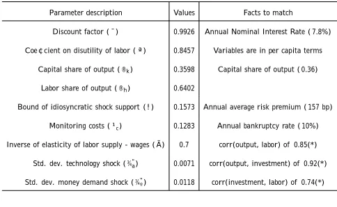
(40) 1.5. Solution method. I follow Campbell [5] in the solution method. The main idea is to linearize the equilibrium conditions arising from the household’s, …rm’s and entrepreneurs’ problems respectively. These conditions are given in the Appendix. At this point Campbell’s method of undetermined coe¢cients is applied. The mechanism is to guess that the rates of growth of variables can be expressed as functions of capital predetermined in period t ¡ 1, Kt ; and the shocks (technology and money demand ones). The whole system can be reduced to three equations, one for the demand for capital, one for the interest rate rule, and the last one for the Euler equation for consumption. Once all the variables are substituted, I only need to solve for the undetermined coe¢cients to obtain the solution paths for the variables.. 1.6. Parameter values. The model parameterization seeks to match empirical observations of postwar US data. Some parameters are calibrated, whereas others are taken from the standard literature. Results are reported in Tables 1:1 and 1:2. The time period considered is one quarter. The parameters or the model are ¯; µ; Ã; ª; ±; ®k , ®h , !; ¹c ; »; as well as those parameters de…ning the stochastic processes of the shocks (½a ; ½º ; ¾ "a ; and ¾ "º ): I will take µ; ±; »; ½a ; and ½º from previous estimates in the literature on business cycle models for the US postwar data. The remaining parameters, that is, ¯; Ã; ª; ®k , ®h , !; ¹c , ¾"a ; and ¾"º are calibrated to match US data. Regarding preference parameters, the discount factor is chosen to match an annual nominal interest rate equal to 7:8% at the non-stochastic steady state, given an average mean money. 23.

(41) _. growth, X; equal to 1:2%; …gures which are consistent with US data. This implies a ¯ equal to 0:9926: To make it easier to get intuition about the dynamics of the model, I will choose preferences so that income and substitution e¤ects cancel out, that is, the relative risk aversion parameter14 is µ = 1. The inverse of the labor supply elasticity with respect to real wages, Ã; is more controversial.15 I give this parameter the value 0:7; that is, the elasticity of labor supply with respect to real wages will be close to 1:5. This elasticity helps the model replicate the empirically observed relative standard deviations reported in Table 1:3; mainly the correlation between output and labor. The coe¢cient ª has been calibrated so that labor in the nonstochastic steady state equals one. This means that all variables are measured in per capita terms: For technology parameters, I take the depreciation rate, ±; to be 2% per quarter, which is consistent with estimates for the US postwar period. The capital share on aggregate income, in the model without credit market imperfections is taken to be 0:36; this implies an ®k equal to 0:3598 in the model with credit frictions. This is computed taking into account that aggregate output, Y A ; equals output plus added value from the capital sector, Y + i[Q ¡ 1]: Notice that in the case without monitoring costs, the price of capital is one, Q = 1; and therefore, Y A = Y: By assuming constant returns to scale in the production function, ®h is obtained, where ®h = 1¡®k . Next, I calibrate parameters related to credit market imperfections. These are the bound on ». the support of the uniform distribution of ! t ; that is, !; and the monitoring costs, ¹c : Following Gertler [18], I keep the elasticity of net worth with respect to output, »; equal to 4:45; which is consistent with US estimates. The bound ! and the monitoring costs ¹c are calibrated to match 14. Although I am not analyzing growth, I prefer to use preferences which are consistent with balanced growth,. as is the case speci…ed here. 15. See for example the paper by Christiano, Eichenbaum and Evans [9].. 24.

(42) _. an annual value for the bankruptcy rate, ©(!t ); of 10%, and an annual risk premium of 157 basis points, measured by the spread between the commercial bank lending rate and the commercial paper rate on average terms16 reported by Fuerst [15]. The resulting values are ! = 0:1573; and ¹c = 0:1283: It remains to specify the stochastic processes of the shock variables. The steady states of all the shocks are normalized to 1. Following traditional literature estimates, the autocorrelation coe¢cient for the technology shock, ½a ; is assumed to be 0:95; consistent with the high persistence of these perturbations observed in the data (King and Rebelo [24], Ireland [23]). For the shock to money demand, estimates for US data show large and highly persistent money demand shocks (Ireland [22]). Thus, I follow Christiano and Gust [10], and set ½º equal to 0:95 also. Given these values, the standard deviations for the shocks are simultaneously calibrated to match several second moments in the data reported in Table 1:3: More concretely, I focus on the correlation of output with investment and the correlation between investment and labor. These correlations have been chosen because they summarize the key mechanism of the models investigated. Mainly, the e¤ects induced by credit market imperfections in the production of investment goods are translated to output through changes in labor. The resulting values are ¾"a = 0:0071; and ¾"º = 0:0118: Finally, when the Taylor rule is at work, I will consider a version of the rule with the following coe¢cients: ° r = 0:66; ° ¼ = 0:61; and ° y = 0:16. This rule is denoted as stable by Christiano and Gust [10] when applied to a limited participation model, in the sense that it determines a stable unique equilibrium.17 This is also the case here. The general consensus in giving a higher 16. There is a wide discrepancy for the values regarding monitoring costs and bankruptcy rates. The reader can. …nd discussion about them in Carlstrom and Fuerst [6], Fisher [13], and Bernanke, Gertler, and Gilchrist [4]. 17. As usual when dealing with interest rate rules, issues regarding indeterminacy of equilibrium arise. In prin-. 25.

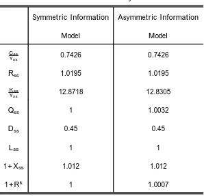
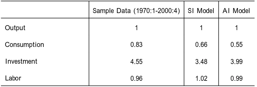
(43) weight to in‡ation smoothing rather than to output stabilization is also followed. Table 1.2 summarizes the steady state values for the two setups considered. In the remainder of the paper I will denote the model without frictions the symmetric information model, ¹c = 0, and refer to the case with frictions as the asymmetric information model, ¹c > 0 (SI and AI, respectively). Recall that when monitoring costs are zero, the model collapses to a standard limited participation framework. Note also that steady state values for some variables di¤er _. between models. However, both start at the same level of 1 + X; which means that policies di¤er only in terms of their cyclical characteristics.. 1.7. Quantitative properties of the models. In this section, I analyze the ability of the two models presented above to account for some stylized facts suggested by the literature on business cycles. Table 1:3 presents some key moment relationships implied by the SI and AI models, and compares them with real US data. For actual US data, the sample selected goes from 1970:1 to 2000:4. The series have been taken from the FRED Database (Federal Reserve Bank of St. Louis) and correspond to Real GNP, Real Personal Consumption Expenditure, Real Gross Private Domestic Investment, and Nonfarm Payroll Employment, in logarithms and detrended using the Hodrick-Prescott …lter. The risk premium is measured as the spread between the Bank Prime Rate and the Six-month Treasurybill Rate. Part A of Table 1.3 presents the relative standard deviations of some variables with respect ciple, there is no reason to assume that the regions characterizing uniqueness, indeterminacy and explosiveness in this model are the same as those obtained by Christiano and Gust [10] for a limited participation framework. Thus, I analyzed indeterminacy for the models in this paper given the rule. The coe¢cients reported here lie in the area of unique equilibrium.. 26.