Approximation of phase-field models with meshfree methods: exploring biomembrane dynamics

APPROXIMATION OF

PHASE-FIELD MODELS

WITH MESHFREE METHODS:

EXPLORING BIOMEMBRANE DYNAMICS

Christian Peco Regales

Doctoral Thesis

Advisor: Marino Arroyo

Barcelona, September 2014

Wayne Gretzky

Approximation of phase-field models with meshfree methods: exploring

biomembrane dynamics

Christian Peco Regales

Biomembranes are the fundamental separation structure in animal cells, and are

also used in engineered bioinspired systems. Their simulation is challenging,

particu-larly when large shape changes and dynamics are involved, or micrometer systems are

considered, ruling out atomistic or coarse-grained molecular modeling. The main goal

of this thesis is to develop a computational framework to understand the dynamics

of biomembranes embedded in a viscous fluid using phase-field models. Phase-field

models introduce a scalar continuous field to define a diffuse moving interface, whose

physics is encoded in partial differential equations governing it. These models can

deal with dramatic shape and topological transformations and are amenable to

multi-physics coupling. However, they present significant numerical challenges, such as the

high-order character of the equations, the resolution of sharp and moving fronts,

or the efficient time-integration. We address all these issues through a

combina-tion of meshfree spacial discretizacombina-tion using local maximum-entropy basis funccombina-tions,

and a Lagrangian variational formulation of the coupled elasticity-hydrodynamics.

The smooth meshfree approach provides accurate approximations of the phase-field

and can easily deal with local adaptivity, the Lagrangian approach naturally extend

adaptivity to dynamics, and the variational formulation enables nonlinearly-stable

robust variational time integration. The numerical implementation of these methods

in a high-performance computing framework has motivated the development of a new

computer code, which integrates state-of-the-art parallel libraries and incorporates

to other scientific problems in a number of collaborations dealing with

flexoelectric-ity, metal forming, creeping flows, or fracture in materials with strongly anisotropic

surface energy.

I would like to express my special appreciation and thanks to my advisor, Prof.

Marino Arroyo. First, for his guidance, support, enthusiasm and fearless attitude

towards research and work. I have deeply enjoyed the vast majority of the projects

we have embraced and also felt his optimism, help and patience at the tough and

un-certain moments that inevitably appear to give value and meaning to any significant

task. Second, I would like to thank him for his priceless example not only within the

professional field but also within the human side. His balanced and flexible way of

dealing with delicate issues regarding the group and the individual has undoubtedly

improved my perception of leadership, managing and education. I am truly indebted

and thankful to the faculty of LaC`aN and Departament de Matem`atica Aplicada III.

In particular, Professors Antonio Huerta, Antonio Rodr´ıguez, Sonia Fern´andez and

Jose Mu˜noz. I met them at the Civil Engineering degree and all of them are

responsi-ble for the seeds that made me love and focus my attention in this new way of doing

science that is Computational Mechanics. Without their motivation and support,

this journey would not have been possible. I would also like to thank the reviewers

of the thesis and the members of the committee for their useful comments and

ad-vice. I am very grateful to the people at LaC`aN for providing such an enjoyable and

stimulating working environment. A very special thanks to my colleagues and friends

at Omega lab. I’ll never forget the guidance, kindness and sense of humor of Adri´an

Rosolen, the neverending but wise and valuable advices of Daniel Mill´an, the deep

conversations with Susanta Ghosh about the ”true flavour of research”, the

rigorous-ness of Mohammad Rahimi inside the lab and his happy view of the life outside, that

wonderful trip to Porto and the “Old Friends” bottle I shared with Amir Abdollahi,

the passion for cleanness, order and beer of Behrooz Hashemian, the enjoyable

con-versations about Catalonia independence with Alejandro Torres and everything that

Bin Li when he does not understand something, the basketball matches of Kuan and

last but not least, that crazy man known as Dimitri Kaurin. My special thanks also

to David Modesto, Ana Tamayo and Cristina Diaz-Cereceda, among other colleagues

of the “far, far side of the Campus”. We spent perhaps too little but truly enjoyable

and genuine time together. I’m going to miss my lunch time with my dear friend

Gonzalo and our hot chocolates in the break of the french course.

I have so much to be grateful for my friends, specially Xavi and David, and my

dear loved ones, my parents, sisters, little brother and brother in law (”Aut viam

inveniam aut faciam!”), who have been a source of unconditional inspiration and

encouragement. During this time I had the privilege of walking through heaven and

hell, and it was in the darkness where I felt you brighter and closer. Life is like

a collective sport, no real success is achieved just by oneself. Thank you for being

my team now and always, everyone of you is a Ph.D. to me. Following with the

sport, let me bewilder yet and again of how much happiness and inspiration could a

pair of blades bring into my existence. Ice and hockey are already part of me, and

so my dear friends Avi (gracias por encontrarme, profeta del hockey!), Judit and

Cristina (hockey girls!), Ram´on, Max, Artur, Octavi, Oriol, Ruth (la campeona),

Sebastian (the doctor), Sebasti´an (el maestro), Anna, Xavi, Carles and Cristina (el

tr´ıo maravilla del staff), Marc (I did it my waaaayyy!!!!!), Petit (locura sobre la pista)

and Jarek (crack!).

And finally I thank to God. Or chaos, or chance or luck or fate or whatever word

that is able to describe an astonishing chain of circumstances that ends up with you

finding a treasure. In my case this treasure has a name and it is Mar´ıaPaz. Thank

you for such many moments that worth a lifetime. “Le vent se l`eve... Il faut tenter

de vivre!”.

Abstract v

Acknowledgments vii

Contents ix

1 Introduction and overview 1

2 Approximation of meshfree phase-field models 9

2.1 Model complexity . . . 9

2.2 Meshfree methods and the Local Maximum Entropy Approximants . . 12

3 Phase-field modeling of biomembranes 17 3.1 An introduction to biomembranes . . . 17

3.2 Vesicle modeling . . . 20

3.3 Vesicle statics: equilibrium shapes . . . 25

3.4 Vesicle dynamics : an adaptive Lagrangian approach . . . 32

3.4.1 Lagrangian phase-field model formulation . . . 33

3.4.2 Numerical approach . . . 38

3.4.3 Numerical results . . . 41

3.5 Complex biological processes : influence of kinetics and adhesion in vesicle shaping . . . 47

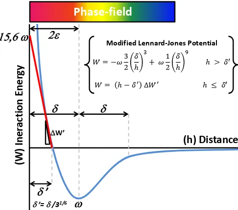
3.5.1 Motivation . . . 47

3.5.2 Modeling adhesion . . . 51

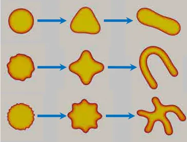
3.6 Kinetics and morphogenesis . . . 55

4 High Performance Computing 59 4.1 Supercomputing: towards an efficient parallel sparse LME environment 59 4.1.1 Neighborhood coarsening algorithm . . . 61

4.1.2 Compressed meshfree basis functions storage . . . 64

4.1.3 Meshfree parallel sparse matrices in PETSc . . . 67

4.2 A brief code overview . . . 70

5.2 A stabilized formulation for viscoplastic flow in metal forming . . . 81 5.3 Computational evaluation of the flexoelectric effect in dielectric solids 84 5.4 Fracture in brittle materials of anisotropic surface energy . . . 89

6 Concluding remarks and future directions 93

6.1 Conclusions and future directions . . . 93 6.2 Publications . . . 95

References and list of figures 97

Appendix A

An adaptive meshfree method for phase-field models of biomem-branes. Part I: approximation with maximum-entropy

approxi-mants. 119

Appendix B

An adaptive meshfree method for phase-field models of biomem-branes. Part II: a Lagrangian approach for membranes in viscous

fluids. 149

Appendix C

Efficient implementation of meshfree Galerkin methods for large-scale problems with an emphasis on maximum entropy

approxi-mants. 177

Appendix D

Meshfree Parallel Algorithms 211

Introduction and overview

Phase-field modeling is a powerful methodology that introduces a scalar continuous

field to describe and connect the different phases of a system. This field, usually called

order parameter, takes constant values in the bulk and gradually changes between

phases naturally identifying an interface. In contrast with classical sharp-interface

methods (see Fig. 1.1), this interface is smeared over a diffuse region, whose thickness

may model a physical phenomenon or result from mathematical regularization.

Phase-field models enable seamless calculations over the bulk and through the

in-terface in a continuous way and thus presents several advantages within a range

of applications that is vast and keeps growing quickly. It has become a corner

stone in material sciences [1, 2], gaining popularity in a wide set of applications

Figure 1.1: Diffuse and sharp-interface approaches. (nele.studentenweb.org)

in applied science and engineering such as fracture [3], microstructure formation and

fracture evolution in ferroelectric materials [4], image segmentation [5], multi-phase

flows [6], infiltration in porous medium [7], shape memory alloys [8] or tumor

angio-genesis [9](see Fig. 1.2). The simulation of biomembrane systems has been a relatively

recent addition in phase-field modeling [10, 11].

First steps of phase-field modeling date back to Van der Waals [12]. In his

ef-forts to understand the density change between a liquid and its vapor, he inferred

from a thermodynamical point of view that the gas-liquid density interface was more

consistent if described as a diffuse transition rather than as a sharp one. These

considerations gave birth to the idea of phase-field or diffuse interface modeling,

which expanded quickly throughout the scientific community, but that was mainly

formalized and developed over the last 50 years. The study of phase transitions

of Ginzburg and Landau [13] in 1963 introduced the fundamental idea of theorder

parameter, which was interpreted as an independent state variable of the

thermo-dynamical system. Hillert [14] applied similar concepts to build the first model for

spinodal decomposition using a discrete phase-field, while Cahn and Hilliard [15]

an-alyzed the same problem by using a continuous phase-field. Ginzburg-Landau and

Cahn-Hilliard made critical contributions to the model, in particular adding to the

mean field free energy (related to the bulk free energy) the contribution of phases

and interfaces and thus giving rise to a consistent free energy functional and a formal

structure to the modern understanding of phase-field modeling. Nevertheless, until

that moment, the concept of a diffuse interface had been built on the purpose of

approaching the physical reality and its properties (i.e. thickness and other related

microscopic parameters) were understood as real and deducible from the energy

po-tentials governing the system.

A second view of phase-field models came to light in 1987 when Langer [16]

real diffusiveness of the interface as well as the related parameters are considered to

be beyond the resolved scale and remain hidden at the microscopic level. Therefore,

the interface thickness becomes a mathematical artifact that mimics the original

sharp-interface model while keeping the phase-field formalism. This viewpoint also

provides a natural route to phase-field model development as a regularization of the

sharp-interface counterpart.

The modeling used in this thesis to simulate biomembrane systems follows this

numerical concept of phase-field i.e. the ratio between the characteristic sizes of

the vesicle radius and thickness is high enough to neglect the physical variations

along the interface. The simulation of these systems with sharp-interface models

poses several difficulties for classical parametrical approaches. From a numerical

point of view, parametric sharp-interface approaches suffer when complex geometries

and topology changes appear, e.g. merging and pinch-off phenomena, which can be

extremely difficult to parameterize. They also run into the necessity of tracking the

interface position at every time step. Many of these problems can be overcome with

phase-field modeling (Table 1.1). Since the interface arises as a change between the

phase-field values, it removes the surface tracking as well as other issues associated

with topological and geometrical difficulties. Of course, phase-field models have

their own drawbacks to be considered. The refinement of the interface, which has

to be resolved, introduces numerical difficulties e.g. the gradually increasing sharp

gradients located on the interface and the resulting stiffness of the system, both in

time and space (we refer to Section 2.1). As a consequence, phase-field models tend

to be computationally expensive.

Some geometrical and topological problems can be tackled with advanced

tech-niques such as subdivision surfaces [17] and level set methods [18]. Level set methods

provide a powerful technique to describe dynamical and complex sharp geometries

com-Table 1.1: Sharp-interface (parametrical) and phase-field modeling comparison.

Aspect/Method Parametrical Phase-Field

Physical field vectorial scalar

Domain line/surface 2D/3D

Interface explicit tracking no tracking

Error sources discretization discretization

interface tracking model

Numerical challenges mesh entanglement local sharp-gradients topological changes adaptivity

plex jump conditions may become difficult. Phase-field models, in contrast, eliminate

these interface conditions and replace them by the order parameter field and a partial

differential equation over the full domain which connects the interface with the rest

of the physical system. Moreover, the connection of the phase-field with the physics

is commonly modeled through a free energy that drives the kinetics of the system,

which makes straight-forward to gradually improve the model by adding contributing

energy terms.

We choose to discretize our Galerkin schemes with the local maximum entropy

(LME) approximants, a meshfree method. These smooth approximants can deal

with the second order derivatives present in many phase-field functionals and handle

local refinement in a robust manner. LME present as well a number of features that

make them suitable for phase-field models, such as their strict non-negativity, the

straightforward imposition of boundary data (they present a weak Kronecker-delta

property on the boundary) and the robustness of their evaluation. The variation

diminishing property is particularly well-suited for phase-field models exhibiting

step-like changes across the interphase.

The main objective of this thesis is to study biomembrane dynamics using

phase-field models discretised with LME approximates. The simulation of biomembranes

(both in space and time) is too expensive for atomistic and coarsed-grained methods

be-havior while keeping the computational cost below reasonable limits. In this thesis

we propose methods that combine different numerical techniques to obtain a robust,

scalable and computationally efficient code. We use a variational approach that

ac-counts for a fourth-order phase-field model describing the vesicle and a dissipation

term to consider the surrounding viscous fluid media. We minimize the action with

respect to the phase field variable in the statics case to get equilibrium shape

solu-tions. In the study of the dynamics we propose a Lagrangian particle method where

we minimize with respect to the deformation mapping of the medium including both

the interface and the background. Since the phase-field is convected by the motion,

the refined regions of the mesh follow the interphase automatically. We extend the

phase-field model to account for adhesion and investigate how confinement and

ki-netics could play a fundamental role in biological membrane shaping, motivated by

recent experiments.

From a computational science perspective, we developed aC+ + code that uses MPI for parallelization and some of the state-of-the-art libraries in scientific

super-computing i.e. PETSc, ParMetis, QHULL, TetGen. We found that meshfree

rou-tines in these packages are not as developed in the field as they are in mesh based

techniques. In consequence, the implementation in supercomputing facilities has

mo-tivated a number of contributions to the implementation of meshfree methods. In

particular, we present an optimization that coarse-grains the connectivity

speeding-up critical algorithms in the system matrix assembly and also a compressed basis

functions storage strategy to overcome memory bottlenecks. The structure of the

resulting library is presented. We briefly report on collaborations in other

prob-lems beyond biomembranes, where the code has been successfully applied due to the

flexible and user-friendly structure of its design.

This thesis is organized as follows. In Chapter 2, we justify the complexity arising

supercomputing. We also give an introduction to meshfree methods in general and

to the LME approximants in particular. We devote Chapter 3 to the phase-field

modeling of biomembranes. We motivate the problem, develop our contributions to

the phase-field modeling of vesicles and briefly introduce our main results in statics,

dynamics and ongoing research. Chapter 4 is a more technical document where

we present a comprehensive description of the C+ + code and point out the main contributions to the implementation of meshfree methods. In Chapter 5 we present

different applications to which we have applied LME and the codes developed in this

work. We finish with some concluding remarks, future research lines and an overview

of the publication record in Chapter 6. The main papers have been referred in the

text and can be consulted in Appendix A, Appendix B and Appendix C. Relevant

Approximation of meshfree

phase-field models

2.1

Model complexity

The main advantage of the phase-field model is the unified treatment of the interfacial

tracking and mechanics, which potentially leads to simple, robust, scalable computer

codes. Additionally, a meshfree method is well-suited to approximate high-order

phase-field models, because the free energy functionals involve high order derivatives.

This combination comes at the expense of a high computational cost, particularly if

the phase-field modeling error with respect to the sharp-interface limit needs to be

small. Furthermore, a meshfree method demands for a higher cost in terms of basis

functions calculation, and suffers from the lack of a mesh-supported connectivity and

heavier sparse matrices and assembly related routines.

In particular, biomembrane phase-field models resort to a 3D scalar PDE to

de-scribe an interphase, which would require a 2D vectorial description in a parametric

representation i.e. while a vesicle surface could be parameterized and resolved in two

dimensions, the phase-field model implies the use of a third dimension to describe

the volume containing the interface. Moreover, the phase-field model accuracy

pends on the diffuse interface resolution, which is controlled by a width parameter

. In biomembrane models, dictates the thickness of the membrane, which should be chosen as small as possible if the target is recovering the sharp-interface limit.

Resolving a smaller implies an even smaller nodal spacing on the discretization grid. In our experience, the nodal spacing h should at least satisfy _≥ 2h. As a consequence, using uniform grids implies a spatial complexity of order O(−d_{) in a}

phase-field model describing an interface of dimension d₋1 embedded in a space of dimension d. This justifies the necessity for adaptive strategies, since the order of complexity can be then ideally lowered one dimension and match the interface

dimension i.e. orderO(1−d_).

Phase-field models introduce a field, which concentrates around a thin layer,

introducing numerical stiffness into the system. This stiffness can be broadly

ex-plained as a property of the system by which large variations in the output arise

from small changes in the input, hence limiting the time step in any explicit time

integration. Furthermore, this type of stiffness arising from different scales is

com-monly reflected by a high condition number in the matrices, thus hampering iterative

solvers, which are in general preferable to treat large sparse matrices. Indeed, it can

be proved that the biomembrane phase-field model produces solutions with the profile

φ(x) = tanhhdist√(x) 2

i

, wheredist(x) is the distance to the interface. Resolving this profile requires a very fine discretization for small values of, but this high resolution is only required in the vicinity of the interface. Away from it, the phase-field is nearly

constant. These issues of phase-field models affect dramatically the performance and

motivate two fundamental choices in the proposed strategy for solving the problems

in this thesis: strong adaptivity and variational time integrators.

The other large source of complexity lies within the meshfree nature of the

ap-proximants used in the discretization. Their choice is motivated by a number of

a more complex structure that can damage the final performance. Approximation of

high-order phase-field models has been previously tackled with other discretization

techniques. Isogeometric analysis [19], a non-negative technology showing precise

ge-ometrical descriptions and the required smoothness to handle high-order operators,

has been successful in approximating phase-field models for a variety of problems

[20, 21]. However, the straight-forward h-refinement and robustness of meshfree

methods in Lagrangian grids under large distortions has motivated the choice of

LME approximants to discretize the biomembrane phase-field models presented in

this thesis. Nevertheless, the non-negative character of these two technologies make

them suitable to be combined to get advantage of their combined strengths [22].

Dis-cretization of PDE’s in a meshfree sparse framework involves a variety of routines

including (i) neighbor search over domain, (ii) computation of the basis functions,

(iii) creation of an sparse matrix structure and (iv) filling of matrix positions with

a particular operation. As discussed in Section 4.1, the last two routines gain

rel-evance as the size of the system increases, and are comparable to the final solver

step, particularly in 3D. The not known a priori structure of the sparse matrices,

the higher density of the connectivity matrix and the large number of integration

points required, introduce a non-negligeable overhead in comparison with standard

mesh-based methods e.g. FEM.

Thus, while mesh free methods provide smooth and flexible approximation for

high-order PDE, these technologies can be computationally demanding, particularly

in conjunction with phase-field models. For this reason, part of this thesis is devoted

2.2

Meshfree methods and the Local Maximum

En-tropy Approximants

Meshfree methods provide an approximation to continuum field equations based on

basis functions that do not rely on a mesh or its connectivity (see [23] for an

intro-ductory review). Therefore, many of the requirements associated with the quality

of the elements in a traditional FEM are relaxed or disappear. This extra

flexibil-ity on the grid of nodes raises new challenges in the numerical implementation [24].

The most popular meshfree approximants are based on the moving least squares

idea [25]. One of the first meshfree methods, the smoothed particle

hydrodynam-ics [26], was originally designed in 1977 to solve astrophysical problems and applied

later to fluid dynamics. From there on, a variety of methods have emerged, such as

reproducing kernel particle method [27], partition of unity finite element method [28]

and element free Galerkin [29] to mention a few. FEM strategies have succeed in

countless computational mechanical and physical applications, but they have also

run into obstacles when facing problems involving discontinuities, sharp fronts, large

distortions and high-order derivatives. Meshfree methods offer several advantages

such as shape functions with high-order continuity, robustness in dramatic grid

de-formations [30, 31] and easier local adaptivity [32, 33]. Most of meshfree Galerkin

methods actually require a quadrature mesh in order to perform integration, and a

higher number of quadrature points to accurately integrate the weak form due to

their non-polynomial nature and non element-wise support. Other issues include

the awkward treatment of essential boundary conditions due to non-satisfaction of

the Kronecker delta property, the computational cost associated to neighborhood

creation to determine the basis functions support and the computation of the basis

functions themselves.

Basis function

Full support Effective support

Tol0

Figure 2.1: Left: Full support of local maximum entropy (LME) basis functions covers the convex hull of the computational domain. The effective numerical support size is given by the truncation errorTol0. Right: Representation of two-dimensional LME approximants. Notice the non-interpolant character and the smoothness of the basis functions, and the fulfillment of a weak Kronecker delta at the boundary of the convex hull.

put forth to develop polygonal approximants [34] and meshfree approximation schemes

[35]. Local maximum-entropy approximants are non-negative and are endowed with

features that are proper to convex approximants, such as monotonicity, smoothness

(C∞, and therefore handle without difficulties high-order derivatives) and variation diminishing property [35]. They satisfy ab initio a weak Kronecker-delta property

at the boundary of the convex hull of the nodes [35] and therefore the imposition of

essential boundary conditions in Galerkin methods is straightforward. Their convex

geometry structure [35] enables the connection with other non-negative technologies

like isogeometric analysis [19] or subdivision surface [36]. Other advantages include

the robustness of their evaluation and a simpler quadrature [37]. Some of these

concepts are illustrated in Fig. 2.1.

Traditional numerical methodologies like finite difference [10, 38] and spectral

methods [39] have been used for phase-field models of biomembranes. Recently,

approximants, has shown an excellent performance for the Cahn-Hilliard equation,

handling successfully the sharp transitions of the solutions without spurious

over-shoots [20, 40]. Although these structured methods can handle higher-order

op-erators, they have difficulties in adapting to localized features. C0 _{finite element} approaches can deal with the high-order character of the functional by reformulating

the model as a system of second order PDE [41] and are well suited for

adaptiv-ity [42], but suffer from poor accuracy for a given computational cost. A number of

adaptive techniques have been developed for the Cahn-Hilliard model, including an

adaptive multigrid finite-difference method [43, 44], a Fourier spectral moving-mesh

method [45], an adaptive FEM with linear [46, 47, 48] and quadratic [49] shape

func-tions after recasting the higher-order phase-field as a system of lower-order equafunc-tions,

and a finite volume approach for unstructured grids [50]. Adaptive methods based

on finite differences [51, 52], Fourier spectral [53], or finite volumes [54, 55] have been

proposed for other higher-order phase-field equations.

Maximum-entropy basis functions, denoted by pa(x), a= 1, . . . , N withx∈Rd,

wheredis the space dimension, are designed to be strictly non-negative and to fulfill the zeroth and first order consistency conditions

pa(x)≥0,

N

X

a=1

pa(x) = 1,

N

X

a=1

pa(x)xa=x, (2.1)

where the last equation allows us to identify the vectorial weightsxa with the

posi-tions of the nodes associated with each basis function.

The idea behind local maximum-entropy basis functions is to construct local

ap-proximants as well as optimal from an information theory viewpoint. It means that

these approximants have to exhibit a (Pareto) compromise between two competing

objectives, minimum width (locality) and entropy maximization (information theory

condi-0 0.5 1 1.5 2 2.5 3 0

0.2 0.4 0.6 0.8 1

γ = [0.6 1.2 1.8 2.4 3 3.6 4.2 4.8 5.4 6]

Figure 2.2: Seamless and smooth transition from meshfree to Delaunay affine basis functions. The transition is controlled by the non-dimensional nodal parametersγa,

which here take linearly varying values from 0.6 (left) to 6 (right).

tions). These requirements enable us to write the following optimization program to

select the approximants

For fixed x, minimize

N

X

a=1

βapa|x−xa|2+ N

X

a=1

palnpa

subject to pa ≥0, a= 1, . . . , N N

X

a=1

pa= 1, N

X

a=1

paxa =x,

(2.2)

where the set of non-negative nodal parameters _{βa = γa/h2a}a=1,...,N defines the

locality of the approximants [35, 56]. The dimensionless parameterγa characterizes

the degree of locality of the basis function associated to the nodexa, whileha

repre-sents the nodal spacing. The basis functions become sharper and more local as the

value of the dimensionless parameter γa increases, and the Delaunay approximants

arise as specialized limits (γa ≥ 4 in the practice), as illustrated in Fig. 2.2 for a

one-dimensional domain.

As fully detailed in [35], it can be mathematically proved that the optimization

problem has a unique solution. The efficient solution follows from standard duality

0 1 2 3 4 5 0 0.2 0.4 0.6 0.8 1 x Basis Functions

0 1 2 3 4 5

−2 −1 0 1 2 x Gradient

0 1 2 3 4 5

−4 −2 0 2 x Hessian

Figure 2.3: One-dimensional local maximum-entropy basis functions (left), and its first and second spatial derivatives (center-right) computed with a dimensionless parameterγ= 0.8.

functions. By analogy with statistical mechanics, we define the partition function

Z(x,λ) =

N

X

b=1

exp₋βb|x−xb|2+λ·(x−xb). (2.3)

At each evaluation point x, the Lagrange multiplier for the linear consistency

condition is the unique solution to a solvable, convex, unconstrained optimization

problem

λ∗(x) = arg min

λ∈Rd

lnZ(x,λ). (2.4)

This optimization problem with d unknowns is efficiently solved with Newton’s method. Then, the basis functions adopt the form

pa(x) =

1

Z(x,λ∗(x))exp

−βa|x−xa|2+λ∗(x)·(x−xa). (2.5)

We refer to [57, 56] for the expressions to compute the gradient ∇pa(x) and

the Hessian matrix Hpa(x) of the local maximum-entropy basis functions, which

are illustrated in Fig. 2.3 for a one-dimensional domain uniformly discretized and a

Phase-field modeling of

biomembranes

In this chapter the main contributions to the simulation of biomembranes are

pre-sented. First, in Section 3.1, we give a brief introduction of biomembranes from a

biological-chemical point of view. In Section 3.2 we go through the theory

under-lying their modeling, and devote Sections 3.3 and 3.4 to modeling and simulation

strategy for statics and dynamics, respectively. Further details can be found in

pa-pers Appendix A and Appendix B. We conclude with a review of the ongoing research

regarding adhesion and confinement phenomena in Section 3.5.

3.1

An introduction to biomembranes

The study of living cells is a very important issue in different fields such as biological

research, medicine and biotechnology. A general feature of all cells is an interface

membrane between the machinery in the interior of the cell and the extracellular

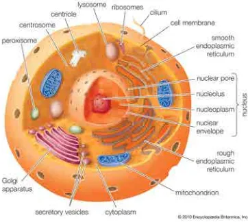
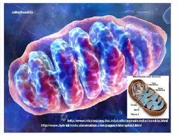
fluid, called the plasma membrane. Eukaryotic cells possess complex compartments

made out of internal membranes, called organelles, instrumental in their function (see

Fig. 3.1), which are also responsible for the transport of substances through cargo

Figure 3.1: Human cell structure. Source: Encyclopedia Britannica Inc.

vesicles or tubes. They also play a key role in bio-mimetic engineered systems [59].

Their complex behavior, rich physical properties, formation and dynamics have been

objects of experimental and theoretical investigation for biologists, chemists and

physicists during many years [60, 61].

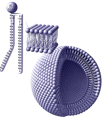
Cell membranes are mainly built from two mono-molecular layers of lipids (called

lipid bilayers) held together by entirely non-covalent forces. They are around 4

nm in the thickness and from tens of nanometers up to millimeters in the

lat-eral directions. Lipids in plasma membranes are chiefly phospholipids e.g.

phos-phatidyl ethanolamine. Phospholipids are amphiphilics with hydrocarbon tails and

hydrophilic polar heads [59, 62, 63]. Therefore, they assemble naturally forming a

hydrostable bilayer, which presents interesting mechanical properties (see Fig. 3.2).

Experimental observations as well as molecular simulations have revealed the

in-plane fluidity of lipid membranes [64, 65] while they behave as flexible solids which

store bending and extensional elastic energies. Upon mechanical loads, lipid bilayers

may be curved, compressed, dilated, or sheared. In the equilibrium state and within

Figure 3.2: Phospholipid bilayer structure and self assembly. (Source: astrobiol-ogy.nasa.gov)

by the following constants: the bending rigidity, the Gaussian curvature modulus,

the area compressibility modulus, and the shear elastic modulus. At physiological

temperatures, most lipid membranes are fluid and therefore lipid membranes have

no strength against shear forces i.e. shear elastic modulus is zero. Below the phase

transition temperature of lipids, lipid membranes form a solid-like gel phase.

Me-chanically, the bilayer acquires a non-zero shear elasticity. In this so-called gel phase,

the relative motion of membrane inclusions is hindered. The fluidity of membranes at

higher temperatures is essential in the case of cellular membranes because it permits

the displacement of membrane anchored macromolecules or inclusions, e.g.

trans-membrane proteins, and provides the necessary malleability for the trans-membrane to

form the intracellular organelles or mediate in tubular and vesicular transport of

proteins (see Fig. 3.3).

The membrane itself, on the one hand, and the surrounding fluid, on the other,

Figure 3.3: Phospholipid bilayer membrane composition. Source: Encyclopedia Bri-tannica Inc.

change, as this involves a rearrangement (and shear) of the lipids and the surrounding

fluid. The resistance or shear in the plane of the film is characterized by the interfacial

shear viscosity of the membrane. One may equivalently define a viscosity related to

the dilation and compression of the membrane. For a complete and more realistic

description of the membranes, one has to consider the existence of two monolayers

which may slip with respect to each other. The intermonolayer slippage is dragged

by a friction force whose amplitude is proportional to the intermonolayer friction

coefficient.

3.2

Vesicle modeling

Vesicles are closed biomembranes, which play an important role in biophysical

pro-cesses such as the delivery of proteins, antibodies or drugs into cells, and separation of

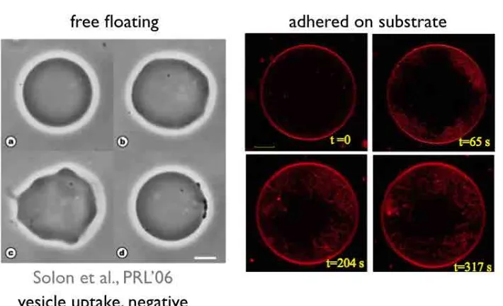
different types of biological macromolecules within cells. Vesicles serve as simplified

models of more complex biological systems, and can be used to study the interaction

between lipid bilayers and the surrounding medium, e.g. under osmotic stress [66],

shear flow [67], or electrical fields [68]. Depending on the lipid composition, lipid

bilayers can phase-separate forming multicomponent vesicles [69], which have also

Atomistic molecular dynamics (MD) simulations have been very useful in the

prediction of the macroscopic characteristics of lipid membranes, but remain limited

to small membrane patches due to the large number of atoms involved in closed

vesicles, and more importantly due to the slow relaxation times of bending modes [70].

As a consequence, the computational cost scales asL6 _{where Ldenotes the lateral} dimension of the system. Coarse-grained simulation, where each particle represents

a number of atoms, can reach larger systems, and there has been notable successful

studies in recent years involving out-of-equilibrium phenomena at the scale of small

vesicles, e.g. [71]. Yet, as in atomistic MD, the scaling of the computational cost

poses a hard upper bound on the system sizes that can be reached with current

computers. Continuum mechanics has been shown to be very efficient in explaining

the statics of lipid bilayers, as well as their dynamics, particularly for large scale

systems [72, 73, 74, 75, 76].

From a mechanical point of view, the fluid vesicle dynamics result from a balance

of elastic forces and two main dissipative mechanisms : the bulk dissipation due to

the drag force of the surrounding fluid and the internal membrane dissipation of lipid

bilayer; likewise, this internal dissipation can be considered to arise from two main

phenomena : the in-plane membrane viscosity and the intermonolayer slippage. We

consider that the elastic behavior of the membrane is dominated by the bending

energy, leaving the extensional energy as a constraint due to its nearly inextensible

behaviour under common forces. Regarding the media, we note that the drag force

of the ambient fluid is dominant at large scales, while at small scales it is negligible

as compared to the surface viscosity. Here we focus on vesicle systems at large scales

(few microns and above), where the mechanics are given by the interplay of bending

elasticity and bulk viscosity (Fig. 3.4).

Therefore, the main effort is put on the continuum description of the coupled

Figure 3.4: Elastic energies and dissipation mechanisms; the model considers the preponderance of bending and solvent in large scale dynamics

to tackle the problem. Nevertheless, other types of dissipation, such as the ones

aforementioned, or the influence of chemical phenomena, such as the protein

con-centrations inducing additional curvature of the membrane, could be added to the

model eventually.

In this study, we are looking for numerically tractable approach for the

simula-tion of complex biological processes involving membranes embedded in a viscous fluid

media, enabling us to examine fundamental questions about cell and organelle

physi-ology. We approach the problem with an innovative continuum description based on a

phase-field model, a meshfree approximation and a Lagrangian framework, resulting

in a variational method that presents automatic adaptivity.

The development of the phase-field model for vesicles starts with the set up of an

order parameter in the spirit of the Cahn-Hilliard [15] approach. In this framework,

we define an order parameterφ(x) that takes values +1 and₋1 to signal the exterior and the interior enclosed volumes of a membrane, respectively. We then find a

in the energy functionals governing the behavior of the system. We follow here

the phase-field model for biomembranes proposed by [10] and developed in [? ],

which start approximating the area and enclosed volume of the vesicle. The volume

description is almost trivial and serves as a primary example of this methodology. It

is clear that the functional,

EV =

Z

Ω

φ dΩ, (3.1)

approximates the difference between the exterior and the interior volumes, and the

functional

EA=

Z

Ω

2|∇φ| 2₊ 1

4(φ

2 −1)2

dΩ, (3.2)

is proportional to the surface area as_→0.

For fluid membranes in our scale range, the main term in the energy functional

was introduced by Canham [77], Evans [78] and Helfrich [79] , which accounts for

the bending elastic energy in a sharp-interface model,

EH=

Z

Γ

_k

H

2 (H−C0) 2_+k

gK+σ

dΓ, (3.3)

where Γ is the surface of the vesicle, H stands for the mean curvature, K for the Gaussian curvature,σrepresents the surface tension,C0is the spontaneous curvature (may be modeled by area difference elasticity [80]) and kH, kg are the bending and

Gaussian rigidities, respectively.

In our model, we let aside the Gaussian curvature term, whose integral remains

constant for a uniform vesicle in the absence of topological changes by virtue of the

Gauss-Bonnet theorem. The surface tension term is also omitted later, because it can

for simplicity C0 = 0, the mean curvature remains as the only contribution to the bending energy.

Under this assumptions, the Helfrich model admits a phase-field formulation [10,

11, 81], where the curvature energy and the associated constraints (area and volume)

of the vesicle can be written as,

E(φ) =fEk

2 Z Ω ∆φ+ 1

φ+C0

√ 2

1−φ2

2

dΩ

V(φ) =1 2

V ol(Ω) + Z

Ω

φ dΩ

=V0

A(φ) =fA

Z

Ω

2|∇φ| 2₊ 1

4(φ

2 −1)2

dΩ =A0

(3.4)

where is a small regularization parameter,fE = ₈√3₂, fA= ₂√3₂, Ω is the domain,

and∂Ω its boundary. The regions _{x:φ(x)>0_}and _{x:φ(x)<0_} represent the inside and outside of the membrane, while the level set_{x:φ(x) = 0_} can be used to realize the position of the membrane. Formal asymptotics [11], as well as rigorous

mathematical analysis [82] (see also [83] for a review), provide the connection between

the phase-field and the sharp-interface models when _→0. As this limit is never achieved in the numerical calculations, a modeling error is always present in practice.

This model has been coupled with the Navier-Stokes equations in [39]. Similar ideas

to couple phase-field models of biomembranes with fluid or other physical fields have

been developed by other researchers as well [68, 84, 38, 46].

Vesicles are always surrounded by a solvent. In most situations of interest, vesicles

evolve in low Reynolds number conditions. The assumption of creeping dynamics lets

us pose the problem from an energetic standpoint and use the dissipation rate from

the energy balance equation to state a variational principle. From the Rayleigh

equations for creeping dynamics.

The Rayleigh dissipation potential for a compressible Newtonian fluid can be

written as

Diss[∂ty;y] = µ

Z

Ω

d0:d0 dΩ +λ 2 Z

Ω

(div v)2dΩ, (3.5)

d0 = d₋¯d= 1

2(∇v+∇v

T₎

−1₃div vI. (3.6)

For an incompressible Newtonian fluid, the second term above is replaced by the

constraint

divv= 0. (3.7)

This expressions allow us to consider the action of the bulk fluid acting on the

vesicle and drive accordingly the dynamics of the system. Considering a slightly

compressible fluid simplifies the mathematical formulation and the numerical

im-plementation. Nevertheless, a numerical treatment of the fully incompressible case

using LME mesh free approximants is described in Chapter 5.

3.3

Vesicle statics: equilibrium shapes

We briefly introduce here the basics for biomembrane statics, which is fully developed

in our paper in Appendix A. In the static approach we aim to minimize the elastic

potential of the vesicle to get equilibrium shapes. These stable configurations have

been widely studied in the biophysical literature, which provides a valuable source

for comparison and validation. At this stage, the objective is to demonstrate that the

numerical scheme proposed to solve the phase-field formulation is able to handle the

different numerical challenges (sharp features, adaptivity, large deformations,

adaptive grids with phase-field models by comparing different levels of refinement

with regular uniform grids. We rely for refinement on Centroidal Voronoi

Tessella-tions [85] to distribute appropriately the nodes based on the phase-field gradient.

In this framework, we simply minimize the elastic bending energy with respect

to the phase-field over a domain Ω containing the vesicle, subject to volume and

area constraints. This minimization leads to different local minima standing for

the different stable shapes. Note that an additional constraint is added in statics,

corresponding to the static moment in the vertical axis (in this work we develop the

formulation in axisymmetric coordinates). This constraint is needed in statics to

control the rigid solid movement in the axisymmetrical axis, and thus prevents the

vesicle from escaping the simulation domain.

We consider the following expansion for the phase-field in terms of the basis

functions

φ(x)_≈φh(x,Φ) = N

X

a=1

pa(x)φa, (3.8)

where Φ = (φ1, φ2, ..., φN) is an array containing the N nodal values of the

phase-field, and we insert this ansatz into the variational problem describing the phase-field

model to obtain the following algebraic optimization program:

Minimize Eh(Φ) =E[φh] =fE

k

2

Z

Ω

W2

h dΩ

subject to Vh(Φ) =V[φh] = 1

2

V ol(Ω) + Z

Ω

φh dΩ

=V0

Ah(Φ) =A[φh] =fA

Z

Ω

2|∇φh| 2₊ 1

4(φ

2

h−1)2

dΩ =A0

Mh(Φ) =M[φh] =

Z

Ω

φh(z−zc)dΩ = 0

φh|∂Ω=−1,

where

Wh=∆φh+

1

φh+C0

√ 2

1−φ2h

. (3.10)

The optimality conditions can be obtained from the Lagrangian function

L(Φ,ν) =Eh(Φ)−νA[Ah(Φ)−A0]−νV [Vh(Φ)−V0]−νM[Mh(Φ)−M0], (3.11)

where the area, volume and static moment constraints are maintained by the

La-grange multipliers or physical reactions ν = (νA, νV, νM), where νA can be

inter-preted as a membrane tension andνV as a pressure difference across the membrane.

After defining a new set of variables x˜ = (Φ,ν) = (φ1, φ2, ..., φN, νA, νV, νM),

the optimal solution of this saddle-point problem can be sought with the

Newton-Raphson method applied to the nonlinear set of equations given by ∂ΦL = 0,

∂νL = 0. However, this approach may lead to mere stationary points, not

mini-mizers of the elastic energy, physically unstable equilibria. Furthermore, given the

difficulty in setting good initial guesses for the Lagrange multipliers, this solution

strategy is not robust. A robust strategy that guarantees stable equilibria is based

on the augmented Lagrangian method, which combines the standard Lagrangian with

penalties. This method retains the exactness of the Lagrange multipliers method and

the minimization principle of penalty methods. The minimization is performed

itera-tively on the phase-field variables for frozen Lagrange multipliers, which are updated

explicitly (see [86, 87] for further details). The augmented Lagrangian is

LA(Φ,ν) =Eh(Φ)−νA[Ah(Φ)−A0]−νV [Vh(Φ)−V0]−νM[Mh(Φ)−M0]

+ 1

2µ|Ah(Φ)−A0|

2

+ 1

2µ|Vh(Φ)−V0|

2

+ 1

2µ|Mh(Φ)−M0|

2

.

We solve the problem in two stages. First, we follow the augmented Lagrangian

method to find an approximate minimizer consistent with the constraints with a

coarse tolerance. Then, this approximation is refined with the regular

Newton-Raphson method on the extended set of variables x. Since the initial guess for˜

this second stage is very close to the actual minimizer, the algorithm never leads to

unstable equilibria. The expressions to compute the gradientsr(˜Φ,ν) and˜rA(Φ,ν)

of the Lagrangian and augmented Lagrangian are lengthy but straightforward, and

can be found in Appendix A.

Numerical results recover stable equilibrium shapes that can be charted in a

phase diagram that has been extensively studied (see [1, 2] and references therein).

This diagram exhibits a number of equilibrium branches, including prolates, oblates,

discocytes, or stomatocytes. The equilibrium shape for a given area, volume, and

spontaneous curvature is not unique in general. For instance, upon deflation of

an initially spherical vesicle without spontaneous curvature, the prolate-dumbbell

and oblate-discocyte branches are possible. Mathematically, the transition shapes

of the equilibrium branches can be tracked by changing the volume constraint and

solving for constrained minimizers. A number of equilibrium shapes for the oblate

equilibrium branch are plotted in Fig. 3.5.

We illustrate the accuracy of the proposed method by analyzing two specific

aspects in axisymmetric examples: (i) the convergence of the phase-field model for

a fixed regularization parameter using uniform grids, and (ii) the convergence of the phase-field model to the sharp-interface model when ( → 0) and the points are adaptively distributed, which is essential to simulate thinner interfaces without

significantly increasing the total number of degree of freedom.

To answer the first question we show in Table 3.1 the numerical energies for

Figure 3.5: 3D views of the oblate equilibrium branch: each shape is computed by minimizing the energy and reducing by 5% the volume of the previous configuration.

Table 3.1: Energies of the discocyte equilibrium shape for different uniform grids of points and several values of. The size of the computational domain is Ω = [0,1.5]_× [0,2]. Reference energy from a sharp interface simulation: Ediscocyte= 9.12657.

ID # nodes ¯h = 0.05 = 0.04 = 0.03 = 0.02 = 0.01

O1 6124 0.024 9.71279 9.59056 – – –

O2 12271 0.017 9.72137 9.59446 9.43775 – –

O3 24597 0.012 9.72671 9.59553 9.43483 9.29532 –

O4 49145 0.0084 9.73203 9.59786 9.43515 9.28938 –

O5 98388 0.0059 9.73536 9.59901 9.43481 9.28674 9.22082

O6 146545 0.0048 9.73716 9.59948 9.43422 9.28378 9.19139

O7 296344 0.0034 9.73989 9.60053 9.43437 9.28326 9.18627

oblate-discocyte branch) and the number of nodes for each grid are indicated in the

first and the second column. As the CVT-generated grids are not perfectly uniform,

the value of the average nodal spacing ¯h is reported in the third column. The re-maining columns show the energies computed for different values of the regularization

parameter. We report the energies only when the transition profile is reasonably resolved, as decided by the relation >2h. Note the energy convergence from above as the number of points increases for each(columns). We can also observe how the value of the energy converges to the sharp interface valueEdiscocyte= 9.12657 as the

Table 3.2: Energies of the discocyte equilibrium shape for several values of and uniform and adapted grids of 6,124 points. Reference energy from a sharp interface simulation: Ediscocyte= 9.12657.

ID # nodes = 0.04 = 0.03 = 0.025 = 0.02 = 0.015 = 0.01

O1 6124 9.59056 – – – – –

O11 6124 9.59678 9.44002 – – – –

O12 6124 – 9.43506 9.35810 9.28849 – –

O13 6124 – – 9.35970 9.28701 9.22588 9.18703

O7 296344 9.60053 9.43437 9.35488 9.28326 9.22399 9.18627

We address now the _→ 0 behavior in adapted grids. As argued in Chapter2, adaptivity is essential for numerical approaches based on phase-field models to be

competitive. A possible strategy for adaptivity is to solve the optimization problem

with a coarse grid of points (and thus a large value of), apply CVT to redistribute the nodes concentrating them around the interface, and compute the phase-field

solution with a smallerfor this new distribution of points. In practice, this strategy cannot be applied at once to get a strong refinement. Indeed, the initial coarse grid

provides an inaccurate phase-field solution, which in turn produces an inadequate

relocation of the points. This ultimately constraints unphysically the phase-field

solutions. A better strategy is to adapt the grid and reduceprogressively.

Table 3.2 reports the bending energies of the discocyte equilibrium shape for

uniform and adapted grids and several regularization parameters. The first and the

last rows correspond to uniform meshes with 6,124 and 296,344 nodes, and are the

same as those reported in Table 3.1. The other rows correspond to adapted grids

with 6,124 nodes, obtained in each step of the progressive adaption of the grid and

reduction of . The first column of the table gives an identification code for the grids of points. A description of the features of each grid is given in Appendix A.

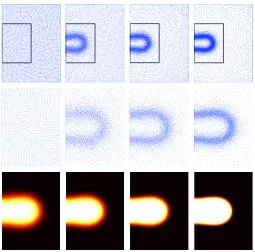
The smooth transition between the successive grids is apparent in the figure, as the

Figure 3.6: Discocyte equilibrium shape. Uniform and adapted grids of 6,124 points (top). From left to right: O1, O11, O12 and O13. Zoom of the areas indicated with black boxes (center). Phase-field (bottom). From left to right, the solutions correspond to= 0.04,= 0.03,= 0.02, and= 0.01.

value for the regularization parameter min for a given grid is determined by the

nodal spacing distribution. As expected, the ability of adapted grids to accurately

support sharp phase-field solutions at an affordable cost is noteworthy. Adapted

grids grant the same accuracy (measured by the optimal energy) as uniform grids

with a 50-fold reduction in the number of degrees of freedom for= 0.01. Figure 3.6 (bottom) shows the equilibrium phase-field for the grids referred to in Table 3.2 and

shown in Figure 3.6 (top, center). It can be noticed that as the value ofdecreases, the thickness of the diffuse interface shrinks considerably.

Further details and numerical examples can be found in the corresponding

3.4

Vesicle dynamics : an adaptive Lagrangian

ap-proach

We introduce here the meshfree Lagrangian method proposed in our paper Appendix

B to study vesicle dynamics. Having shown that the adaptive meshfree method based

on the local maximum entropy approximants can yield very accurate solutions at

an affordable cost for a phase-field model for biomembranes, we turn now to the

(creeping) dynamics of vesicles embedded in a viscous fluid. The adaptive method

proposed in Section 3.3 is adequate to analyze very accurately a given equilibrium

configuration, but is not as well-suited to study quasi-statically equilibrium branches,

as these exhibit buckling events, i.e. very large shape transitions for a small change

in the enclosed volume for instance. The adapted grid for a given state cannot

represent the solution for a very different state, as the high resolution is tailored to the

initial state. Over-damped dynamics or gradient flows, even without a clear physical

meaning [88, 89, 90], can be used to numerically obtain equilibrium shapes, and the

method we proposed here can be interpreted in this vein. Furthermore, the dynamics

of vesicles embedded in a viscous fluid is of interest by itself (see for instance [91] for

a state of the art parametric method for vesicles combined with a boundary integral

method for the Stokes equations with spherical harmonic approximants). Generally,

the inertial effects can be disregarded, and here we consider the low Reynolds number

limit.

Phase-field models for bio-membranes have been coupled with fluid dynamics by

various authors [84, 83]. In all previous approaches, Eulerian framework was adopted,

and a transport equation for the phase-field was set in place. If these models are

combined with adaptivity, cumbersome mesh projection steps will be needed. In

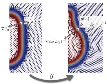
contrast, we propose here a meshfree Lagrangian method to study the dynamics of

• The phase-field is viewed as a material property of the continuous medium, and

the elastic energy changes as this field is pushed-forward by the deformation.

The deformation rate produces viscous forces. The dynamics result from the

balance of the configurational forces of the phase-field elastic energy and the

viscous forces, subject to area or volume constraints.

• Due to the Lagrangian nature of the method and the stability of membrane

structures, if the initial grid is adapted, the adaptivity automatically follows the

sharp features of the solution, although sporadic remeshing steps may become

necessary.

• The variational structure of the problem is fully preserved by the discretization

schemes, which allows us to use robust incremental minimization implicit

time-stepping schemes, which are non-linearly stable by construction.

• The smoothness of the basis functions allows us to treat in a straightforward

way the second order derivatives of the elastic energy functional.

• The meshfree approximants can deal robustly with large deformations of the

fluid/bio-membrane continuum. However, the basis functions can be updated

by reconnecting the nodes along the simulation.

• The method is the same in 2D or in 3D, and is easily made parallel.

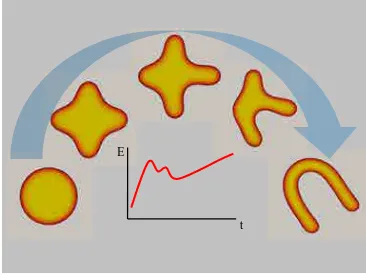
A visual description of the method is shown in Fig. 3.7. The proposed method shares

common features with the optimal mass transport (OTM) method presented in [92].

3.4.1

Lagrangian phase-field model formulation

Consider a fixed fluid domain Ω, where a membrane is located and described at time

y

r

r

(

Dy

)

x

0

(

x

)

y

(

₌

x

)

0

y

1

as described in previous sections). Consider now a motion of the continuum medium,

i.e. a smooth bijective mapping on Ω at each instant of time, yt(x). Viewing the

phase-field as a material property, attached to the material particles, it is pushed

forward by the simulation following

φt(x) =φ0◦yt−1(x) =φ0 y−t1(x)

. (3.13)

From this point on, we omit the explicit dependence on t of the motion and the pushed-forward phase-field. The elastic energy of the membrane in terms of the

phase-field can be computed as

E= 3 8√2

k 2 Z Ω ∆φ+ ₁

φ+C0

√ 2

1₋φ2

2

dΩ. (3.14)

The enclosed volume and surface are can be computed as

V =1 2

V ol(Ω) + Z

Ω

φ dΩ

(3.15)

and

A= 3 2√2

Z

Ω

2|∇φ| 2₊ 1

4(φ

2 −1)2

dΩ. (3.16)

To compute the spacial derivatives of the phase-field, we recall Eq. (3.13) and the

inverse function theorem to obtain

∇φ= ∇φ0F−1◦y−1, (3.17)

whereF=Dyis the deformation gradient. To compute the Laplacian of the

pushed-forward phase-field, we resort to indicial notation and omit the composition with the

relation∂iφ=∂Iφ0F_Ii−1 we have

∂ij2φ◦y=∂IJ2 φ0FIi−1F−

1

Jj +∂Iφ0∂jFIi−1. (3.18)

Now, fromF_Ik−1FkJ =δIJ, we obtain

∂jFIi−1=−F−

1

InF−

1

Ji F−

1

Kj∂KFnJ =−FIn−1F−

1

Ji F−

1

Kj∂

2

JKyn. (3.19)

In particular, we have

∆φ_◦y=∂2

IJφ0FIi−1F−

1

Ji +∂Iφ0∂iFIi−1. (3.20)

Thus, inserting these two equations into the above functionals and pulling-back the

integration by the deformation map, it is clear that they can be interpreted as

func-tions of the deformation mapping, depending parametrically on the initial phase-field:

E[y] = 3 8√2

k

2

Z

Ω

∆φ◦y+ ₁

φ0+C0

√ 2

1−φ20

2

det(F)dΩ, (3.21)

V[y] = 1 2

V ol(Ω) + Z

Ω

φ0det(F)dΩ

, (3.22)

and

A[y] = 3 2√2

Z

Ω

2|∇φ0F −1

|2₊ 1 4(φ

2 0−1)2

det(F)dΩ (3.23)

Lengthy but otherwise straightforward calculations allow us to compute the

varia-tions of these functionals with respect to the deformation. It is obvious that if the

configuration mapping turns to be the identity, the expression for initial phase-field

description is recovered. We can apply this push-forward to the remaining terms

in our problem, such as the dissipation potential. To simplify the exposition of the

penalized formulation of the incompressible Stokes equations.

Following standard continuum mechanics definitions, the Eulerian velocity field

can be computed as

v=∂ty◦y−1. (3.24)

Consequently, the velocity gradient tensor can be written as

∇v_◦y= ˙FF−1, (3.25)

where ˙FiI=∂I∂tyi, and the rate-of-deformation tensor in the Lagrangian domain as

d_◦y=1 2

˙

FF−1_+F−T_F˙T_{. (3.26)}

The Rayleigh dissipation potential for a compressible Newtonian fluid can therefore

be written as [93]

Diss[∂ty;y] = µ

Z

Ω

d:ddΩ +λ 2 Z

Ω

(div v)2 dΩ

= µ

4 Z

Ω

FF˙ −1+F−TF˙T2(detF)dΩ +λ

2 Z

Ω

h

trace( ˙FF−1)i2(detF)dΩ. (3.27)

whereµis the shear viscosity of the fluid, and byDiss[∂ty;y] we highlight the

para-metric dependence of the functional on the current deformationy. The coefficientλ

can be interpreted here as a penalty parameter enforcing incompressibility

approx-imately. For an incompressible Newtonian fluid, the second term above is replaced

by the constraint

tr( ˙FF−1) = 0, (3.28)

We apply the following variational principle [94] to describe the motion of our

coupled problem system, arising from the minimization of a generalized potential

expressing the competition between elastic forces and bulk friction forces,

Diss[∂ty;y] +δE[∂ty;y], (3.29)

with respect to∂tysubject to the constraints

δA[∂ty;y] = 0. (3.30)

If the surrounding fluid is incompressible, the following constraint can be added

δV[∂ty;y] = 0. (3.31)

3.4.2

Numerical approach

The numerical discretization of the variational principle 3.29 in spatial domain using

LME approximants is straight-forward and it is detailed in Appendix B. However, we

note here two additional issues regarding the time discretization and the reconnection

strategies. While minimizing the action and then applying the discretization leads to

a system of nonlinear differential algebraic equations that can be solved with standard

algorithms, the system is stiff because of the nature of the curvature energy, and

because of the presence of constraints. We find that standard numerical packages have

serious difficulties in dealing with these equations, and require very small time-steps

when the system is significantly out of equilibrium. Instead, we develop variational

time-incremental integrators, which can robustly deal with large time-steps. Let us

nodal positions

˙ y≈y

n+1_−yn

∆t , (3.32)

and for the rate of change of the energy

˙

E=E(y

n+1₎

−E(yn₎

∆t . (3.33)

We can then discretize in time the action, and givenyn _findyn+1 _{by minimizing}

1 2(y−y

n₎T_K(yn_)(y

−yn) + ∆tE(y) (3.34)

with respect toy, subject to

Ah(y) =A0, (3.35)

where K is the stiffness matrix resulting from the Galerkin discretization of the Stokes

equations, providing a discrete dissipation potential that depends onyn_{, see Eq. 3.27.}

In the expression we have multiplied the action by ∆t2 _{and ignored the constant}

E(yn_{) in Eq. (3.34). This method is related to the backward-Euler method, and}

many other variational integrators can be defined by choosing different

time-discrete approximations of the action. The resulting nonlinear optimization program

can be solved with a variety of methods. Here, we impose the constraints with

Lagrange multipliers and solve the first order optimality conditions with Newton’s

method. We also note that, by construction, E(yn+1₎

≤E(yn_{), and therefore the}

method is endowed automatically with nonlinear stability. We note that adaptive

time-stepping algorithms can be easily designed, for instance adapting ∆tin such a way that ∆E is nearly constant. The adaptivity may also be driven by the number of iterations needed in the nonlinear solver.

y(ˆx↵)

ˆ

x↵

x

Reset the reference configuration

y(x) =X

a

pa(x)ya

y

The basis functions are defined by the reference set of nodes

pa(x)

x

y

ˆ

x

y(ˆ

x

)

w↵ (detF)w↵

(r 0)↵ (r 0F 1)↵ (@IJ2 0)↵ Eq. (3) Reference configuration

Recompute with the new set of nodespa(x)

Figure 3.8: As the Lagrangian simulation proceeds, the deformation may significantly distort the domain. To avoid this, we periodically reset the reference configuration, as shown in the figure. This involves reseting the reference node position to the current position, recomputing the meshfree basis functions from the new node set, which involves new neighbor searches as indicated with the colored regions, and reseting the quadrature points ˆxα_{, the corresponding weights, and the reference phase-field first}

and second derivatives as indicated in the figure. Note that the reference phase-field value at the quadrature points,φα

0, does not need to be updated as the phase-field is a material property and the quadrature points keep their material identity.

adaptivity is advected by the Lagrangian map, and therefore local refinement along

the dynamics is accomplished for free. The Lagrangian framework allows us to

pull-back the successive states of the system to a reference configuration. Thus, we avoid

the calculation of the meshfree basis functions in every step of the evolution. It has

been shown that the meshfree method considered here can withstand significant

de-formation before the discretized dede-formation mapping ceases to be injective (i.e. the

Jacobian determinant becomes negative at a quadrature point) [35]. However, we

avoid coming close to this limit, which degrades the accuracy of the