remote sensing
ISSN 2072-4292 www.mdpi.com/journal/remotesensing ArticleAutomatic Detection and Classification of Pole-Like
Objects in Urban Point Cloud Data Using an Anomaly
Detection Algorithm
Borja Rodríguez-Cuenca 1,*, Silverio García-Cortés 2, Celestino Ordóñez 2 and Maria C. Alonso 1
1 Department of Physics and Mathematics, University of Alcalá, Campus Universitario Ctra.,
Alcalá de Henares, 28871 Madrid, Spain; E-Mail: [email protected]
2 Department of Mining Exploitation, University of Oviedo, Escuela Politécnica de Mieres,
Gonzalo Gutiérrez Quirós, 33600 Mieres, Spain; E-Mails: [email protected] (S.G.-C.); [email protected] (C.O.)
* Author to whom correspondence should be addressed; E-Mail: [email protected]; Tel.: +34-918-856-748.
Academic Editors: Juha Hyyppä, Devrim Akca, Parth Sarathi Roy and Prasad S. Thenkabail
Received: 28 July 2015 / Accepted: 17 September 2015 / Published: 28 September 2015
Abstract: Detecting and modeling urban furniture are of particular interest for urban management and the development of autonomous driving systems. This paper presents a novel method for detecting and classifying vertical urban objects and trees from unstructured three-dimensional mobile laser scanner (MLS) or terrestrial laser scanner (TLS) point cloud data. The method includes an automatic initial segmentation to remove the parts of the original cloud that are not of interest for detecting vertical objects, by means of a geometric index based on features of the point cloud. Vertical object detection is carried out through the Reed and Xiaoli (RX) anomaly detection algorithm applied to a pillar structure in which the point cloud was previously organized. A clustering algorithm is then used to classify the detected vertical elements as man-made poles or trees. The effectiveness of the proposed method was tested in two point clouds from heterogeneous street scenarios and measured by two different sensors. The results for the two test sites achieved detection rates higher than 96%; the classification accuracy was around 95%, and the completion quality of both procedures was 90%. Non-detected poles come from occlusions in the point cloud and low-height traffic signs; most misclassifications occurred in man-made poles adjacent to trees.
Keywords: pole-like objects; feature extraction; pattern recognition; clustering; 3D point cloud; MLS; anomaly detection
1. Introduction
Creating and updating accurate maps and spatial databases has been demanded by various applications such as city management, urban planning, and intelligent transportation systems. For city management and urban planning, accurate land cover information is needed to document cities growth, make policy decisions, and improve land use planning [1]. For intelligent transportation systems, updated geodatabases that include the location of urban objects and traffic signs are required for terrestrial navigation and, of course, to decrease traffic congestion, lessen the risk of accidents [2], and develop autonomous driving systems [3]. Geospatial information has been widely used to meet these requirements for accurate and up-to-date remote sensed data. Light detection and ranging (LIDAR) technology has been used extensively in surveying and mapping. This technology provides three-dimensional data that complements the spectral information contained in two-dimensional images. Laser scanner sensors can be placed on aerial (airborne laser scanner, ALS) and terrestrial platforms (terrestrial LIDAR). Terrestrial LIDAR can be subdivided into two types: static and dynamic. Static terrestrial LIDAR technology (terrestrial laser scanner, TLS) data is collected from a sensor fixed in a base station. Thus, a small area can be mapped with high accuracy, but several scans are needed to cover large areas. Dynamic terrestrial LIDAR sensors (mobile laser scanner, MLS) are installed in vehicles provided with, as for ALS platforms, a navigation system based on global navigation satellite systems (GNSS) and inertial measurement units (IMUs). These devices determine the position of the mobile platform and the direction and orientation of the sensor at every moment [4].
Given that MLSs and ALSs capture data in large areas within short periods, both sensors are commonly used for urban applications, while the TLS is reserved for short-range applications, such as forest inventory [5], deformation monitoring [6] or heritage documentation [7]. ALS and MLS sensors provide three-dimensional (3D) point cloud data from mobile platforms, but significant differences exist between the two systems. ALS capture objects from the top view, while MLS and TLS collect data from the side-view, which makes the data taken by both types of sensors complementary. Additionally, the distance between the sensors and the ground is shorter in an MLS than in an ALS; consequently, the former performs measurements with higher resolution and greater density than the aerial sensors. ALS sensors cover large areas cost-effectively and rapidly but fail to capture details of small urban targets. Thus, MLS sensors are suitable for ground-based object modeling and to detect and extract elements located at street level, hardly achievable tasks in low density ALS data [8]. The main disadvantage is that MLS output files are large and hard to manage, forcing the development of organizing, cataloging, and optimizing methodologies to reduce the computation time significantly.
approach, the point cloud is decomposed into several two-dimensional vertical slices using the global positioning system (GPS) time as auxiliary information [11] or into horizontal sections, parallel and above the ground [12]. Other works analyze each scan line individually instead of considering the cloud as a whole [13,14]. Removal of parts of the cloud that belong to objects that are not the focus of the study [15] is another common technique. A segmentation procedure is also routinely used for point cloud handling. Segmentation is the process of grouping the points of the cloud into segments: points in the same region are given the same category and treated as a set [16]. Some segmentation techniques such as graph cut [17], region growing [18], and 3D connected components [19] are also applied to facilitate the handling of the point cloud.
In our approach a fully automated method for detecting pole-like objects and classifying them as trees and man-made poles is developed. This method detects and classifies vertical urban elements from MLS data by means of a three step procedure:
1. A preprocessing stage, including a reference frame transformation and a region of interest (ROI) isolation. These procedures diminish the size of the original point cloud, the number of false positives in the following procedures, and the computational effort of the successive stages. 2. Vertical urban elements detection using the Reed and Xiaoli (RX) anomaly detection
algorithm. Previously the preprocessed point cloud is organized in a pillar structure.
3. Vertical elements classification into two classes (trees and man-made poles) using an unsupervised classification algorithm.
2. Method
2.1. Preprocessing
Three-dimensional point cloud data files from MLS data systems include not only X, Y, and Z point coordinates but also additional information such as GPS time, scan angle, or reflectance intensity information, for the millions of points contained in the point cloud. In the current paper, the preprocessing step is divided into two main stages: (i) transforming the reference frame and (ii) removing the parts of the cloud that are not of interest in this work (point cloud reduction).
2.1.1. Reference Frame Transformation
Point clouds registered by MLS sensors are properly geo-referenced in a global reference system by a navigation system (GNSS) and an IMU, which provide coordinates within a global frame to every registered point. The original coordinate system is now transformed by means of a translation and three rotations into a local Cartesian coordinate system. The origin of the new reference frame is located at the beginning of the MLS trajectory, the z-axis is coincident with the local vertical direction, and the x-axis is coincident with the average direction of the vehicle. The y-axis completes the dextro-rotatory set, which makes local (x,y,z) coordinates handier than the global ones.
2.1.2. Removing Uninteresting Points
Geometric Index Definition
To identify the façades of the point cloud, a geometric index was developed. Indexes developed from geometric features of the cloud have been adopted in previous works such as [33], in which an operator based on a normal vector was introduced as a preprocessing step of an object recognition procedure. The index elaborated in the current paper is called the Geometric Index (GI) and combines the information provided by the normal vector and roughness values of every point of the cloud:
𝐺𝐼𝑖 = |𝑁𝑋𝑖| + |𝑁𝑌𝑖| − |𝑁𝑍𝑖| |𝑁𝑋𝑖| + |𝑁𝑌𝑖| + |𝑁𝑍𝑖| ×
1
𝑒𝑅𝑖 (1)
In Equation (1) (𝑵𝒙𝒊, 𝑵𝒀𝒊, 𝑵𝒁𝒊) are the components of the normal vector 𝑵⃗⃗ in the point 𝑷𝒊 and 𝑹𝒊 is the roughness of the studied point. These values are measured from those points contained in a sphere of radius r centered in the studied point (𝑷𝒊). Roughness (𝑹𝒊) is defined as the distance between the
studied point 𝑷𝒊 and the least square best fitting plane comprising 𝑷𝒊 and its neighborhood points inside the radius r sphere [6]. The first term of Equation (1) combines the three elements of the normal vector in a single value normalized in [–1, +1]. The behavior of the normal vector and its sensitivity to variations in the neighborhood size have been analyzed in five urban element types, easily identified in urban environments: façades, treetops, poles, roads, and cars. Significant differences have been found between these elements. In those elements with a horizontal flat surface that are determined as a trend surface (mainly roads and sidewalks), the vertical normal component (𝑵𝒁𝒊) takes higher values than the horizontal ones 𝑵𝑿𝒊 and 𝑵𝒀𝒊. The opposite occurs on façades and fences, which are best fitted by vertical
surfaces, in which horizontal normal vector components (𝑵𝑿𝒊 and 𝑵𝒀𝒊) take greater values than the vertical one. Other elements such as trees or cars present an irregular appearance because of their irregular and heterogeneous shapes. The roughness is included in the denominator of the second term of the GI Equation as an exponential to improve the separation between flat and rough surfaces. The lowest roughness values correspond to flat surfaces while higher roughness values take place in those elements with irregular shapes. According to the roughness study shown in Figure 1a, roughness 𝑹𝒊 takes values around 0m in flat elements and higher values in rough surfaces; thus, term 𝒆𝟏𝑹𝒊takes values around one for flat surfaces and lower in points that are further from the fitted plane. Consequently, the second term will not significantly affect the value of the GI in flat elements but will notably reduce it in rough surfaces, which helps to identify these elements in the point cloud. Since 𝒆𝑹𝒊 is close to one for flat
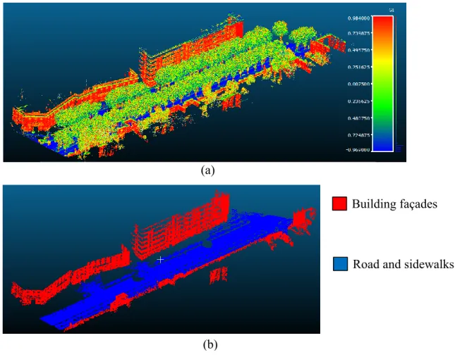
and (ii) the processing time is acceptable. In Figure 1, the roughness and the GI with different neighborhood sizes are shown. These studies were conducted in the two test sites. Figure 1a shows that the lowest roughness values correspond to flat surfaces; while higher roughness values correspond to the elements with irregular shapes. According to Figure 1b, the highest GI values, close to one, correspond to building façades and the lowest, around –1, to surfaces such as roads or pavement. Figure 2a shows the GI of the point cloud used as test site B in a color palette in which red corresponds to higher GI values, close to one, blue is reserved for the lowest GI values, and yellow and green represent the points with an intermediate GI value, around zero.
Figure 1. Behavior of the roughness (a) and GI (b) in five street elements for different neighborhood radii.
Extraction of Vertical and Horizontal Surfaces
To extract the vertical and horizontal surfaces, two thresholds α𝑉 and α𝐻 are set on the GI index. Those points (P𝑖) with a higher 𝐺𝐼𝒊 than α𝑉 are considered to belong to a vertical surface; meanwhile, points with a GI𝑖 below α𝐻 are treated as horizontal surfaces. Point clouds obtained after thresholding
are composed of vertical and horizontal surfaces but also by points that satisfy these conditions that do not belong to these surfaces. These points are usually isolated or belong to small urban elements, such as treetops or pole-like objects.
The 3D-connected components were segmented in favor of (i) grouping the points that belong to the same surface and (ii) removing isolated noisy points. Connected components analysis scans an image and labels its pixels into components if they are connected to each other (either four or eight connected) [34]. Once all groups have been determined, each pixel is labeled with an identifier according to the component the pixel was assigned to [35]. This technique is adapted to 3D point clouds structured in octrees. In a similar manner as for 2D images, the 3D connected components analyze the connectivity of the octrees and group in the same segment those that have a common side. In this case, the 3D connected components segmentation is defined by two parameters: the octree level (OL) and the minimum number of points per segment (MINP). The OL is related to the size of the octrees in which
-1 -0.8 -0.6 -0.4 -0.2 0 0.2 0.4 0.6 0.8 1
5cm 10cm 36cm 50cm 100cm 150cm 200cm 250cm
GI for different elements and neighborhood radii 0.0 m 0.1 m 0.2 m 0.3 m 0.4 m 0.5 m 0.6 m 0.7 m 0.8 m
5cm 10cm 36cm 50cm 100cm 150cm 200cm 250cm
Roughness for different elements and neighborhood radii
(a) (b)
Façades Roads Pole
s
the point cloud is organized. It must be large enough for every octree not to be empty of points but sufficiently small for different urban elements to belong to independent octrees. A priori knowledge of the point cloud density is required to set the appropriate OL. Optimal OL has been empirically established, by the authors, as five times the mean distance between the points of the cloud. The MINP determines the number of components and their size. The objective of this step is removing isolated noisy points, and only large segments that represent building façades and pavement are considered. Once the 3D connected components are segmented, the entire segments recognized as façades are grouped into a single point cloud. This operation is repeated for the segments that represent roads, resulting in three point clouds: the original measured by the MLS sensor, one containing points that belong to building façades, and one with roads and sidewalks information (Figure 2b).
Figure 2. (a) GI in test site 2 and (b) façades detected after the connected components segmentation.
Original Point Cloud Reduction
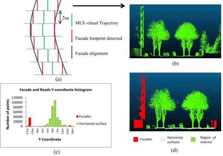
The isolated region coming from preceding procedures that represents the road is analyzed using two-meter-wide sections, perpendicular to the x-axis of the local reference frame (Figure 3a). For each section, the center of the road and the location of building façades at both sides of the street are determined by analyzing the histogram of these point clouds. In every section, the road center is considered the modal class value in the y-coordinate histogram of the horizontal surfaces point cloud (Figure 3b). Thus, it is possible to approximately recreate the path followed by the MLS sensor, providing a kind of virtual MLS trajectory by joining the pavement center detected in each section.
(a)
(b)
Additionally, for every 2-m-wide section, the alignment of the existing buildings is established by searching the modal class values of the y-coordinate histogram at both sides of the road center. A new point cloud is then generated by removing the points that lie beyond the façade line at both sides of the street (Figure 3d). This procedure automatically reduces the volume of the original point cloud, speeding up the following processes and removing potential false positives caused by vertical building columns. Furthermore, since this method is applied in narrow sections 2 m wide, it also accurately and precisely eliminates building façades in curved street sections or difficult areas, such as road intersections.
Figure 3. (a) Cloud MLS analysis in two meters width sections; (b) Original point cloud; (c) Histogram of façades and horizontal surfaces extracted and (d) Point cloud reduced: Isolated region of interest in green and removed façades in red.
2.2. Pole-Like Elements Detection 2.2.1. Point Cloud Structuring
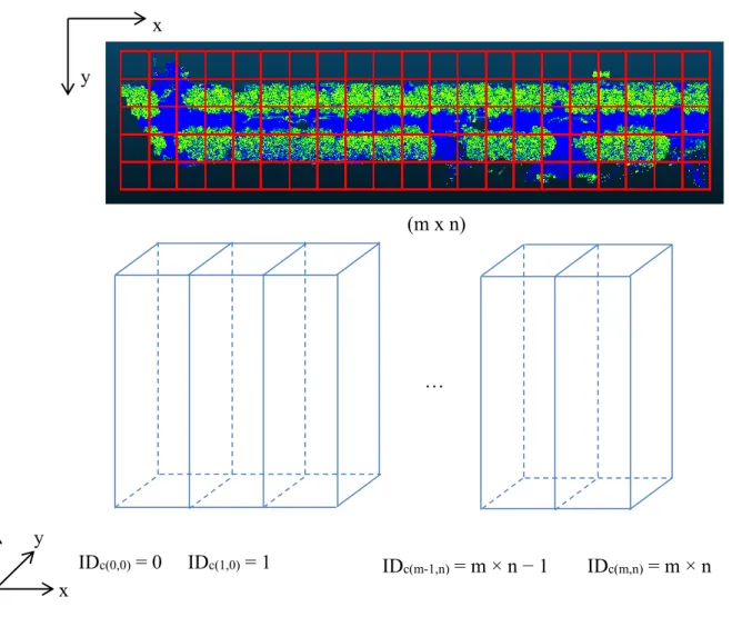
MLS data is composed of several million points so analyzing every single element and its neighborhood is computationally expensive and unproductive in terms of feature extraction. To speed up the detection and extraction procedure, the point cloud obtained in the previous step is organized and analyzed in a 3D vertical pillar structure pattern (Figure 4) [36].
Every point of the cloud is associated with a pillar, and all the points belonging to the same pillar are considered a set. The point cloud is divided in a 2D (m × n) grid composed of m columns and n rows.
0 20000 40000 60000 80000 100000 120000
-17
m
-13
m
-9m -5m -1m 3m 7m 11m 15m 19m
Nu
mb
e
r
of p
oin
ts
Y-Coordinate
Facade and Roads Y-coordiante histogram
Facades
Horizontal surface
Region of interest
Facades Horizontal
surfaces MLS virtual Trajectory
Facade footprint detected
Facade alignment
(b)
(c) (d)
2m
Each cell of the grid represents a pillar. Every pillar has a unique identifier ID assigned from its (x,y) coordinates in the 2D grid. Thus, for every cell ci = (xi, yi), with xi∈ [0, m] and yi∈ [0, n] corresponds
the identifier IDc = (m × yi + xi).
Figure 4. Creation of the pillar structure in the studied point cloud.
Figure 5. Pillar height is delimited until an empty voxel is found.
To avoid considering pillars as infinitely tall elements, the point distribution in each pillar is analyzed. This is achieved by decomposing the pillars into voxels of regular heights. The process starts searching the lowest occupied voxel, that is, the voxel with the lowest height that contains at least one point, and continues studying the voxels above it until an empty voxel is detected. Once a discontinuity is observed,
IDc(0,0) = 0 IDc(1,0) = 1 IDc(m-1,n) = m × n − 1 IDc(m,n) = m × n
(m x n)
… x
y
x z
that is, the first empty voxel above the occupied ones, the points above the discontinuity, if any, are discarded and not considered in the following steps. Thus, every pillar is formed by the points whose z-coordinate is between the lowest occupied voxel and the first discontinuity (empty voxel), found in the pillar. After this operation, every pillar is formed only by the elements connected to the ground level and disconnected points that unnecessarily increase the weight of the pillar and may hinder the detection and classification process are removed (Figure 5).
2.2.2. RX Anomaly Detection Algorithm
Once the point cloud has been structured, vertical urban elements are extracted and classified from the pillars in which the point cloud has been decomposed. It is necessary to determine which pillars contain a target element and which not. The RX anomaly detection algorithm is applied with this goal. This algorithm is commonly used to detect outliers in hyperspectral images, but it can also be used in multispectral images. The RX algorithm was developed by Reed and Xiaoli Yu [37]. It is based on the Mahalanobis distance and follows Equation (2) [38]:
𝛿𝑅𝑋(𝑃𝑖) = (𝑟𝑖 − 𝜇)𝑇𝐾𝐿𝑋𝐿−1(𝑟𝑖 − 𝜇) (2)
where 𝒓𝒊 is a vector in which considered features in the studied pillar 𝑃𝑖 are saved, μ stores the mean values of the considered variables in the set of pillars of the whole point cloud, K is its sample covariance matrix, and L is the number of considered variables. i is the number of pillars in which the point cloud is structured. The minimum value of i is zero (the first studied pillar) and the maximum value depends on the size of the considered pillars The Mahalanobis distance is used to calculate how far each pillar is from the center of the cloud formed by the other pillars, and the shape of the cloud is considered through K. Mathematically, the RX algorithm performs some kind of inverse procedure of the principal component analysis (PCA); this was proved by Alonso et al. [39]. Anomalies should be understood as those elements whose spectral signature differs from the terrain in which they are. Anomalies are significant features of special interest to image analysts. In a hyperspectral image, every band contains information from a certain wavelength of the electromagnetic spectrum. The RX algorithm detects those pixels for which, in any band of the hyperspectral image, exists an anomalous spectral response compared with the response of the rest of the pixels of the image. MLS point clouds do not provide spectral information, but some geometric features can be computed for each point and its neighborhood. These geometric features have singular behaviors in vertical elements, quite different from other street elements.
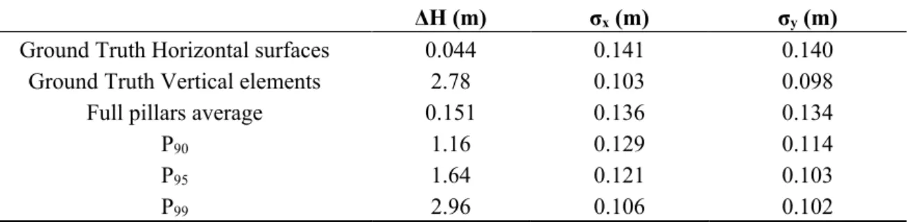
In this work, the RX algorithm is applied to three features for every pillar of the point cloud. Height difference and the points’ spatial dispersion have been considered to detect those pillars that represent a vertical urban element. To study the behavior of street objects in the variables, pillars that represent horizontal surfaces and vertical elements were chosen as ground truth (Table 1).
can be seen in Table 1, the average value for the height difference in the full set of pillars is close to the trend of horizontal elements, with a low height difference (around 0.15 m).
Spatial dispersion is calculated from x- and y-coordinate dispersion (σx, σy). The distribution of the
(x,y) coordinates of the points contained in every pillar depends on which element is contained in it. The standard deviation of both planimetric coordinates (x,y) are the dispersion measures used as a geometric feature. In Table 1, the average (x,y) dispersion in roads and pavement is around 0.14 m; in pole-like elements, the average dispersion is a bit lower, around 0.10 m.
The number of points contained in every pillar (density) in which the point cloud is organized has been used in other works as a feature for extracting urban objects with satisfactory results [40]. Furthermore, surfaces that are orthogonal to the laser pulses show a higher density than those that are nearly parallel [11], a useful property for differentiating orthogonal from parallel elements. However, in the current work the accumulative number of points in every pillar was discarded and not included as a feature for detecting vertical elements. This is because the number of points that represent an urban element depends on the relative position of every element in relation to the MLS sensor and on the laser scanner properties. The same urban furniture located at both sides of the street does not have the same number of points in the 3D dataset even though they correspond to the same type of element. The closer an element is to the sensor, the more points represent it in the point cloud. Incorporating the point accumulation as a descriptor in an automatic detection procedure may cause errors in the process due to the different behavior of the elements shown in the point cloud.
To determine the relationship between the RX values and the features, the correlation between these variables was studied (Table 2). The RX values and height differences had a high positive correlation (0.72); meanwhile, the RX and both dispersions presented a negative correlation (–0.44 for 𝛔𝑿 and
–0.57 for 𝛔𝒀). The pillars with a ΔH higher than the average and dispersions (𝛔𝑿 and 𝛔𝒀) lower than the average have higher RX values. In Table 1, the mean value of the features (ΔH, 𝛔𝑿, 𝛔𝒀) in three RX
percentiles (P90, P95, and P99) are shown. As the correlation study suggested, the higher the RX values, the higher the ΔH and the lower the 𝛔𝑿 and 𝛔𝒀. The pillars included in the RX 99th percentile are
considered vertical urban elements since they perform a behavior similar to that of vertical elements’ ground truth.
Table 1. Behavior of horizontal surfaces and pole-like elements in the considered features and average values among the full set of pillars and in percentiles 90, 95, and 99 of RX values.
ΔH (m) σx (m) σy (m)
Ground Truth Horizontal surfaces 0.044 0.141 0.140
Ground Truth Vertical elements 2.78 0.103 0.098
Full pillars average 0.151 0.136 0.134
P90 1.16 0.129 0.114
P95 1.64 0.121 0.103
Table 2. Correlation matrix between RX and considered geometric features.
ΔH σx σy
RX 0.72 −0.44 −0.57
2.3. Pole-Like Elements Classification
Once the vertical pole-like elements are extracted they are classified into two categories: man-made poles and trees. In this step each detected vertical element is isolated from the rest and treated as an independent set of points. The correct selection of descriptors is a key point to obtain good results in the classification procedure. In our case three descriptors for vertical element were computed: the roughness of their points (both mean and dispersion values) and the scattering of radial distance (𝝆) of the cylindrical coordinate frame centered in the studied pole-like set of points.
Cylindrical coordinates: After the reference frame transformation performed in the preprocessing step, the point cloud is referred to a local coordinate system. In the current step a new reference frame transformation is performed for every detected pole, moving from the Cartesian local reference frame (x,y,z) to a cylindrical coordinate system (ρ, ϕ, z). For every detected pole-like object its own cylindrical coordinate frame system is established. Its cylindrical axis coincides with the direction of Z-axis in the local coordinate system and it is located in the (x,y) centroid of the set of the points that belong to the pole-like object. From the cylindrical triplet of coordinates, the most interesting feature to accomplish this classification is the radial distance (𝛒𝑷). This is because points that belong to man-made poles are closely located around the vertical cylindrical axis than those that represent trees due to their thin appearance. Thus, the dispersion of 𝛒𝑷 in these elements is lower than in trees.
Roughness: It has been observed that both mean and standard deviation of roughness have a different behavior in each category, being their values significantly differ in both types of pole objects. Roughness values of artificial poles are lower than trees due to their flat and smooth shape on their upper part, contrary to the irregular and rough appearance of treetops, which cause higher values on these descriptors. Additionally, dispersion of this parameter in poles is lower than in trees due to the heterogeneity caused by branches and treetops
In order to test whether the geometric descriptors taken into account are distinguishable and present a distinctive behavior in the two considered classes, a separability study has been carried out. To achieve this inspection a ground truth has been generated by identifying diverse elements of both categories in the point cloud. There are several methods to measure the separability between variables; in this work Jeffries-Matusita (JM) distance and transformed divergence, computed from Bhattacharyya distance (BD) (3) has been used as separability measure [41]. In Equation (3), (µ𝒂, µ𝒃) and (𝝈𝒂, 𝝈𝒃) are, respectively, the
𝐵𝐷 =1
8× (µ𝑎− µ𝑏)2× 2 (𝜎𝑎2+ 𝜎𝑏2)
+1
2 × log(
𝜎𝑎2+ 𝜎 𝑏2
2 × 𝜎𝑎× 𝜎𝑏) (3)
𝐽𝑀 = 2 × (1 − 𝑒−𝐵𝐷) (4)
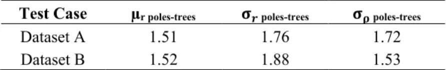
Table 3. Jeffries-Matusita distances for man-made poles and trees in the considered descriptors: mean and standard deviation of roughness (µr and σ𝑟) and standard deviation of ρ (σρ).
Test Case µr poles-trees 𝛔𝒓 poles-trees 𝛔𝛒 poles-trees
Dataset A 1.51 1.76 1.72
Dataset B 1.52 1.88 1.53
3. Test Cases
The efficiency of the proposed method was tested in two datasets measured by different MLS sensors. In every test site the detection and classification procedure have been performed in order to test the capability of the proposed method to extract and classify pole-like objects.
3.1. Mapping Data 3.1.1. Dataset A
The point cloud used as test site 1 represents a 300 m section of an urban street in Boadilla del Monte, a city in western Madrid, Spain. This street is a type of a wide boulevard, with two lanes for each direction, the tracks of a tram in the median strip, and sidewalks and parking areas on both sides of the street. Features such as trees, shrubbery, traffic lights, lampposts, containers, bus shelters, pedestrians, or vehicles are present in this scene. This dataset was selected to test the method in areas of the city with wide streets and a great variety of vertical elements. The slope, 5% on average in this street section, also affected the selection of this test site. This dataset comprises more than 3 million points and was acquired with the IP-S2 Compact + system produced by Topcon Inc. The IP-S2 incorporates a dual frequency GNSS receiver, an IMU, and a connection to external wheel encoders, which receive odometry information. These three systems provide a highly-accurate 3D position for the vehicle. The IP-S2 Compact + scanner is equipped with five laser scanners that collect 150,000 points per second at a range of 40 m, with a vertical field of view of 360°. It is also equipped with a panoramic camera that delivers 360° spherical imagery.
3.1.2. Dataset B
via differential GPS post-processing after data collection using GPS base station data [42]. In this case, the point cloud was composed of more than 6 million points, and the measurements were made along a 400-m-long street in Busto Arsizio, in the Lombardy region, in northern Italy. The street is narrow, and there is one lane in each direction and sidewalks, parking areas, and buildings on both sides of the road. Furthermore, there is a double barrier of leafy tall trees on both sides of the road that causes occlusions in urban furniture, such as lampposts or traffic signs present in this test site. This site was chosen to test the efficiency of the method in narrow streets covered by dense woody vegetation.
3.2. Reference Data
A ground truth was created in each of the two datasets in order to evaluate the results provided by the detection and classification procedures. The target elements included in the detection ground truth database are those with a pole-like shape, among which are lampposts, traffic signs, traffic lights, and trees. In the classification reference data, pole-like objects are sorted into two categories: man-made poles and trees. The reference datasets were composed of all the pole-like elements that were identifiable in the original point cloud. Ground truth in Dataset A is composed of 241 pole-like objects; 141 were man-made poles and 100 were trees. In Dataset B, a total of 228 pole-like elements were observed; 56 were trees and 172 artificial poles.
The validity of our model was quantified by means of completeness, correctness and quality quantifiers, which follow Equations (5)–(7), respectively [43]. TP (true positive) are the detected poles that matched the reference, FP (false positive) represents the detected poles that do not match the ground truth, and FN (false negative) symbolize the poles that exist in the ground truth but are not detected by the proposed method.
𝐶𝑜𝑚𝑝𝑙𝑒𝑡𝑒𝑛𝑒𝑠𝑠 = 𝑝𝑜𝑙𝑒𝑠 𝑚𝑎𝑡𝑐ℎ𝑒𝑑 𝑡ℎ𝑒 𝑟𝑒𝑓𝑒𝑟𝑒𝑛𝑐𝑒 𝑝𝑜𝑙𝑒𝑠 𝑜𝑓 𝑟𝑒𝑓𝑒𝑟𝑒𝑛𝑐𝑒 =
𝑇𝑃
𝑇𝑃 + 𝐹𝑁 (5)
𝐶𝑜𝑟𝑟𝑒𝑐𝑡𝑛𝑒𝑠𝑠 = 𝑝𝑜𝑙𝑒𝑠 𝑚𝑎𝑡𝑐ℎ𝑒𝑑 𝑟𝑒𝑓𝑒𝑟𝑒𝑛𝑐𝑒 𝑒𝑥𝑡𝑟𝑎𝑐𝑡𝑒𝑑 𝑝𝑜𝑙𝑒𝑠 =
𝑇𝑃
𝑇𝑃 + 𝐹𝑃 (6)
𝑄𝑢𝑎𝑙𝑖𝑡𝑦 = 𝑝𝑜𝑙𝑒𝑠 𝑚𝑎𝑡𝑐ℎ𝑒𝑑 𝑡ℎ𝑒 𝑟𝑒𝑓𝑒𝑟𝑒𝑛𝑐𝑒
𝑒𝑥𝑡𝑟𝑎𝑐𝑡𝑒𝑑 𝑝𝑜𝑙𝑒𝑠 + 𝑢𝑛𝑚𝑎𝑡𝑐ℎ𝑒𝑑 𝑟𝑒𝑓𝑒𝑟𝑒𝑛𝑐𝑒 =
𝑇𝑃
𝑇𝑃 + 𝐹𝑃 + 𝐹𝑁 (7)
To quantify the results of the classification step, the classification ground truth was compared with the labeled point cloud provided by the clustering algorithm. For every test site, a confusion matrix was constructed from which five parameters well-known in the evaluation of classification procedures are extracted: overall accuracy, commission and omission errors, and user and producer accuracy [44].
3.3. Algorithm Settings
analyzed in order to establish the range of values that every parameter can take without affecting the final result of the procedure (Table 4). Regarding RX percentile, which is the parameter that determines the pole-like objects detection, its influence in the extraction has been studied and quantified for different percentile values in order to determine the optimal ones. It has been concluded that RX percentile values that provide the best quality rates are P98.5 and P99 (Table 5).
In the current work, the GI thresholds were set from the studies summarized in Figure 1, in which the vertical surfaces (façades) were detected for αV > 0.8 and horizontal elements (pavement and sidewalks)
were located when αH > −0.8. Thus, the vertical and horizontal surfaces were set to GIi > 0.8 and
GIi < −0.8, respectively. Regarding the 3D connected components segmentation, the MINP was set to
2000 points/region. For the octree level (OL), in the cases the mean distance between points was almost 4 cm, which implies an OL of 20 cm. Other parameters, such as pillar size and RX, are less dependent on the characteristics of the cloud and had similar values in every case because they refer to the properties of pole-like urban elements. For the test sites used in this work, the pillar size was established at 50 × 50 cm, and the RX percentile was fixed at P99. The same settings were applied to both test sites (Table 4).
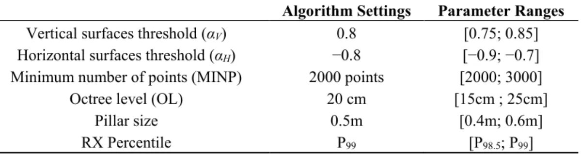
Table 4. Algorithm settings used in the test sites A and B and range of values that every parameter can take.
Algorithm Settings Parameter Ranges
Vertical surfaces threshold(αV) 0.8 [0.75; 0.85]
Horizontal surfaces threshold(αH) −0.8 [−0.9; −0.7]
Minimum number of points (MINP) 2000 points [2000; 3000]
Octree level (OL) 20 cm [15cm ; 25cm]
Pillar size 0.5m [0.4m; 0.6m]
RX Percentile P99 [P98.5; P99]
4. Results
4.1. Dataset A
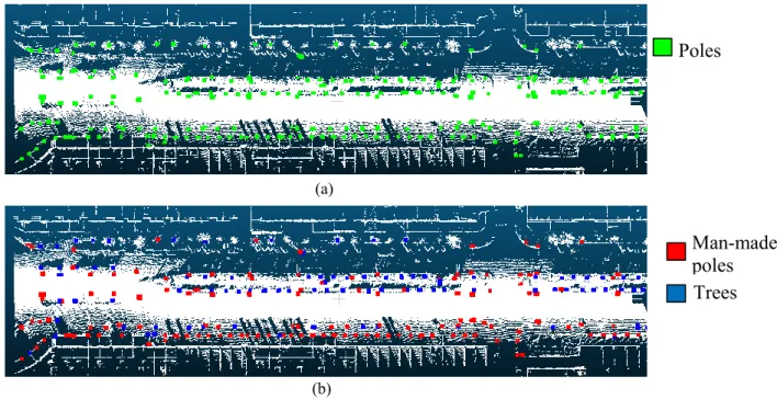
In the point cloud corresponding to this dataset, 241 pole-like elements have been observed among trees, lampposts, traffic signs, traffic posts, and tram posts. The detection procedure extracts 233 vertical elements (Figure 6a), of which 230 match with the ground truth reference and the three remaining detected poles correspond with a working vehicle that has a similar structure to the pole-like objects (Figure 7e). Consequently, eleven poles were undetected, nine of them due to their position in occluded or shadowed regions of the point cloud (Figure 7c). The two others non-detected poles are traffic signs of low height included in the reference dataset, but not high enough to be extracted by the method (Figure 7a,b). According with these results, the detection step takes completeness, correctness, and quality rates of 95.4%, 98.7%, and 94.3%, respectively (Table 5).
8.6%, respectively. In relation to poles, five of 137 man-made poles included in the ground truth reference were incorrectly labeled. These poles are close to trees and their branches modify the appearance of the artificial poles, providing a scattered shape more characteristic of trees than of its own nature (Figure 7f,g). This classification results in a commission and omission errors of 5.71% and 3.65%, being the producer’s and user’s accuracy achieved 96.35% and 94.29%, respectively (Table 6). In an overall evaluation of detection and classification procedures, 217 pole-like objects out of 241 were correctly detected and classified, which means an accuracy of 90.04% (Table 7).
Figure 6. Results for the detection (a) and classification (b) procedure in Test Site 2.
Table 5. Completeness, correctness and quality achieved with the proposed detection method in the two studied test sites with different RX percentile values.
Test Site A/
RX Percentile Observed Detected FP FN TP Completeness Correctness Quality
97.5 241 347 111 5 236 97.93 68.01 67.05
98 241 314 78 5 236 97.93 75.16 73.98
98.5 241 252 17 6 235 97.51 93.25 91.09
99 241 233 3 11 230 95.4 98.7 94.3
99.5 241 144 2 99 142 58.92 98.61 58.44
Test Site B/
RX Percentile Observed Detected FP FN TP Completeness Correctness Quality
97.5 228 359 136 5 223 97.81 60.43 61.26
98 228 314 91 5 223 97.81 68.83 69.91
98.5 228 244 21 5 223 97.81 91.39 89.56
99 228 222 2 8 220 96.5 99.1 95.7
99.5 228 119 1 110 118 51.75 99.16 51.53
Trees Man-made poles Poles detected
(a)
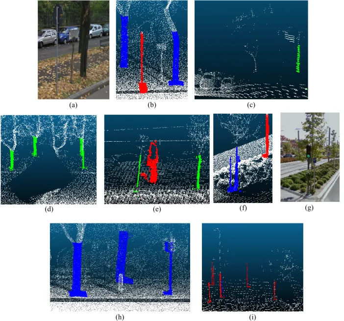
Figure 7. (a,b) little signals appearance in a RGB image and in the point cloud, (c,d) occlusion of a tree trunk, (e) in red, features detected in a work vehicle, (f,g) man-made pole surrounded by tree branches in a RGB image and in the point cloud, (h) rough and scattered man-made traffic light wrongly classified as a tree, and (i) tree with scarce and sparsevegetation misclassified as a man-made pole.
Table 6. Confusion matrix of the classification procedure in test site A, where columns are the ground truth and rows represent the classification results.
Dataset A Trees Poles Σ
Trees 85 5 90
Poles 8 132 140
Σ 93 137 230
Overall Accuracy = 94.35% (217/230)
(a) (b) (c)
(d)
(i) (h)
Table 6. Cont.
Dataset A Commission Omission Trees 5.56% (5/90) 8.6% (8/93)
Poles 5.71% (8/140) 3.65% (5/137)
Producer’s Accuracy User’s Accuracy Trees 91.4% (85/93) 94.44% (85/90)
Poles 96.35% (132/137) 94.29% (132/140)
Table 7. Quality evaluation complete procedure in Dataset A and B.
4.2. Dataset B
In this street section, 228 vertical elements were observed of which 220 were correctly extracted, eight were undetected, and two were falsely detected. Thus, the completeness of the detection procedure was higher than 96%, the correctness above 99%, and the quality higher than 95% (Figure 8a,b and Table 5). Regarding the eight false negatives, the undetected elements, seven were discarded by the method because they were a special kind of traffic sign, with a lower height than ordinary signs (Figure 7a,b). The remaining missing pole element corresponded to a tree trunk, which was partially occluded in the point cloud by a parked van (Figure 7d). The two false positives were detected from the structure of a van that had a shape similar to pole-like objects, with high height differences and low dispersion in (x,y) coordinates. The number of non-target pole-like elements detected would have increased, especially inside the footprint of buildings, unless the original point cloud reduction step had not been carried out. In relation to the classification step, in this road section the overall accuracy rate was 95.0%, which means that 209 out of 220 vertical elements were correctly labeled (Figure 8c,d). According to Table 8, ten man-made poles were mistakenly labeled as trees. Six of these poles were surrounded by branches of nearby trees, which caused the scattered and rough appearance of their pole in the cloud. The remaining four poles were low traffic lights, which were misclassified due to the roughness generated by their upper light structure (Figure 7h). Only one tree was wrongly classified as an artificial pole. The shape of this tree was similar to a pole, with a thin, tall trunk and barely scattered branches. These results provide a commission and omission rate of 6.02% and 0.63% in the trees and 1.85% and 15.87%, respectively, in the man-made poles category. For accuracy, tree classification achieved a producer accuracy of 99.36% and a user accuracy of 93.98%; meanwhile, the pole labeling was 84.13% and 98.15% in the producer and user accuracy, respectively (Table 8). Thus, 209 vertical elements out of 228 were correctly detected and labeled, which meant a global accuracy of 91.67% of the complete procedure (Table 7).
Observed Detected FP Undetected Correctly Labeled
Wrongly
Labeled Accuracy Test site A 241 233 3 11 217 13 90.04 (217/241)
Table 8. Confusion matrix of the classification procedure in Dataset B, where columns are the ground truth and rows represent the classification results.
Dataset B Trees Poles Σ
Trees 156 10 166
Poles 1 53 54
Σ 157 63 220
Overall Accuracy = 95.0% (209/220)
Dataset B Commission Omission Trees 6.02% (10/166) 0.63% (1/157)
Poles 1.85% (1/54) 15.87% (10/63)
Producer’s Accuracy User’s Accuracy Trees 99.36% (156/157) 93.98% (156/166)
Poles 84.13% (53/63) 98.15% (53/54)
Figure 8. A zenithal and perspective view of the detection (a,b) and classification (c,d) results achieved with the proposed method in dataset B.
(b)
Detected Poles
Trees Man-made poles
(c)
4.3. Comparison with Previous Methods
The results provided by our method were compared with other algorithms to evaluate its performance. In the current literature, several methods focus on extracting urban objects. In [15] the target elements were lampposts; trees were the main category in [27], and [23] extracted all types of pole-like objects without differentiating between different types. The lack of a common dataset with a ground truth associated means that every work uses its own dataset and creates a ground truth with visual inspections of the field and the point cloud. In [23] a method for extracting pole-like objects is presented that achieves a completeness detection rate average of 92.3% and a correctness of 83.8% in the four datasets. Most false positives obtained by this method are detected inside the footprint of buildings. The method developed by [30] achieved completeness and correctness rates of 77.7% and 81.0%, respectively, for targets closer than 30 m to the scanner route, which means a mean accuracy of 79.3%. Only when targets closer than 12.5 m were considered, these rates increased, achieving 83.5% and 86.5% for completeness and correctness, respectively, and a mean accuracy of 85%. Most failures in the remotest parts of the clouds were due to shadowed areas and low point density in these areas. [32] extracted lampposts in six datasets achieving completeness rates above 99% and correctness between 97.55% and 99.01; the quality index ranged from 96.74% to 98.21%. Despite the high accuracy, this method seems to be far from automated due to the large number of thresholds to be set to conduct the extraction. Individual street trees were extracted in [29] and accuracy rates above 98% were achieved. This method presents some limitations because it is designed to be used in flat terrains, and all trees must be the same height from the ground. Furthermore, this method achieves accurate results in individual street trees, but its effectiveness in dense vegetated areas where treetops are merged has not been tested. In [26], the accuracy in pole-like objects recognition was 63.9%, and in [31] the completeness and correctness achieved in detecting individual trees ranged from 80.7% to 81.2% and from 70.2% to 75.5%, respectively.
The pole-like object detection method proposed in this paper achieved quality rates in the two datasets of 94.3% and 95.7%, respectively, which are slightly higher than some of the previous methods. The two datasets used to test this method were measured by different sensors in diverse scenarios, which prove its robustness. This algorithm is independent of the scanning geometry and of the slope of the street because the coordinates are transformed in the preprocessing step. In addition, this process detects the horizontal and vertical surfaces in the point cloud and automatically delimits the regions of interest, thus avoiding false positives inside the footprints of buildings. Furthermore, this process does not require a priori information or previous training, and the number of thresholds has been minimized in order to automate the procedure. However, certain problems may occur in remote areas of the cloud with low point density and in trees whose trunks appear tilted. A previous work [30] proposed the development of methods for separating tree trunks from other poles. In the current work, trees and man-made poles were distinguished with a clustering algorithm. This classification procedure achieved an overall accuracy higher than 90% in every data case.
5. Conclusions and Future Works
detection of pole-like objects by means of an anomaly detection algorithm and their classification in trees and man-made elements without prior training data, and (iii) the definition of a robust procedure that can be easily automated and provides accurate results with minimal user intervention.
The pole-like object detection method proposed in this paper achieved quality rates in the two datasets of 94.3% and 95.7%, respectively, which are slightly higher than other methods. The two datasets used to test this method were measured by different sensors in diverse scenarios, which prove its robustness. This algorithm is independent of the scanning geometry and of the slope of the street because the coordinates are transformed in the preprocessing step. In addition, this process detects the horizontal and vertical surfaces in the point cloud and automatically delimits the regions of interest, thus avoiding false positives inside the footprints of buildings. Furthermore, this process does not require a priori information or previous training, and the number of thresholds has been minimized in order to automate the procedure. However, certain problems may occur in remote areas of the cloud with low point density and in trees whose trunks appear tilted.
The typology and casuistry of urban pole-like objects are very diverse, and there is probably no single best method for detecting and classifying them in all cases. According to the results in this work, we can conclude that this method is robust, useful for automatically detecting and classifying pole-like objects, and provides satisfactory results regardless the heterogeneity of the area and the specifications of the sensor and does not need the knowledge of the measured MLS trajectory. In the future, other anomaly detection algorithms could be tested in the detection step, and other features such as laser intensity could be introduced in the classification procedure to expand the classification to other types of urban elements. The detecting procedure provided quality values of around 95% in two test sites, and the classification step achieved an overall accuracy above 94%. In an overall evaluation of both procedures, more than 90% of the vertical elements were correctly detected and classified.
Acknowledgments
The authors would like to thank the Optech Inc. and TOPCON Inc. for providing the datasets to test the proposed method.
Author Contributions
The authors, Borja Rodríguez-Cuenca, Silverio García-Cortés, Celestino Ordóñez and Maria C. Alonso, designed the research, performed data analysis, and contributed with ideas, writing and discussion.
Conflicts of Interest
The authors declare no conflict of interest.
References and Notes
1. Mundia, C.; Aniya, M. Analysis of land use/cover changes and urban expansion of Nairobi city using remote sensing and GIS. Int. J. Remote Sens. 2005, 26, 2831–2849.
3. Levinson, J.; Askeland, J.; Becker, J.; Dolson, J.; Held, D.; Kammel, S.; Kolter, J.Z.; Langer, D.; Pink, O.; Pratt, V. Towards fully autonomous driving: Systems and algorithms. In Proceedings of IEEE Intelligent Vehicles Symposium (IV), Baden-Baden, Germany, 5–9 June 2011; pp 163–168. 4. Jiang, X.; Bunke, H. Fast segmentation of range images into planar regions by scan line grouping.
Machine Vis. Appl. 1994, 7, 115–122.
5. Hyyppä, J.; Jaakkola, A.; Chen, Y.; Kukko, A. Unconventional LiDAR mapping from air, terrestrial and mobile. In Proceedings of the Photogrammetric Week, Stuttgart, Germany, 9–13 September 2013; pp 205–214.
6. Zogg, H.; Ingensand, H. Terrestrial laser scanning for deformation monitoring—Load tests on the Felsenau Viaduct (CH). Int. Arch. Photogramm. Remote Sens. 2008, 37, 555–562.
7. Rüther, H.; Held, C.; Bhurtha, R.; Schröder, R.; Wessels, S. Challenges in heritage documentation with terrestrial laser scanning. In Proceedings of the 1st AfricaGEO Conference, Capetown, South Africa, 30 May–2 June 2011.
8. Zhu, L.; Hyyppa, J. The use of airborne and mobile laser scanning for modeling railway environments in 3D. Remote Sens. 2014, 6, 3075–3100.
9. Vosselman, G.; Gorte, B.G.; Sithole, G.; Rabbani, T. Recognising structure in laser scanner point clouds. Int. Arch. Photogramm. Remote Sens. Spat. Inf. Sci. 2004, 46, 33–38.
10. Douillard, B.; Underwood, J.; Kuntz, N.; Vlaskine, V.; Quadros, A.; Morton, P.; Frenkel, A. On the segmentation of 3D LiDAR point clouds. In Proceedings of IEEE International Conference on Robotics and Automation (ICRA), Shanghai, China, 9–13 May 2011; pp 2798–2805.
11. Yang, B.; Fang, L.; Li, J. Semi-automated extraction and delineation of 3D roads of street scene from mobile laser scanning point clouds. ISPRS J. Photogramm. Remote Sens. 2013, 79, 80–93. 12. Rodríguez-Cuenca, B.; García-Cortés, S.; Ordóñez, C.; Alonso, M.C. An approach to detect and
delineate street curbs from MLS 3D point cloud data. Autom. Constr. 2015, 51, 103–112.
13. Jaakkola, A.; Hyyppä, J.; Kukko, A.; Yu, X.; Kaartinen, H.; Lehtomäki, M.; Lin, Y. A low-cost multi-sensoral mobile mapping system and its feasibility for tree measurements. ISPRS J. Photogramm. Remote Sens. 2010, 65, 514–522.
14. Lehtomäki, M.; Jaakkola, A.; Hyyppä, J.; Kukko, A.; Kaartinen, H. Performance analysis of a pole and tree trunk detection method for mobile laser scanning data. Int. Arch. Photogramm. Remote Sens. Spat. Inf. Sci. 2011, 38, 197–202.
15. Yujie, H.; Xiang, L.; Jun, X.; Lei, G. A novel approach to extracting street lamps from vehicle-borne laser data. In Proceedings of 19th International Conference on Geoinformatics, Shanghai, China, 24–26 June 2011; pp 1–6.
16. Rabbani, T.; van den Heuvel, F.; Vosselmann, G. Segmentation of point clouds using smoothness constraint. Int. Arch. Photogramm. Remote Sens. Spat. Inf. Sci. 2006, 36, 248–253.
17. Golovinskiy, A.; Funkhouser, T. Min-cut based segmentation of point clouds. In Proceedings of IEEE 12th International Conference on Computer Vision Workshops (ICCV Workshops), Kyoto, Japan, 27 September–4 October 2009; pp 39–46.
19. Verma, V.; Kumar, R.; Hsu, S. 3D building detection and modeling from aerial LiDAR data. In Proceedings of IEEE Computer Society Conference on Computer Vision and Pattern Recognition, New York, USA, 17–22 June 2006; pp 2213–2220.
20. City of Melbourne Street Furniture Plan. Available online: http://www.melbourne.vic.gov.au/ (accessed on 22 June 2015).
21. Rabbani, T.; Van Den Heuvel, F. Efficient hough transform for automatic detection of cylinders in point clouds. In Proceedings of ISPRS Workshop: Laser Scanning 2005, Enschede, The Netherlands, 12–14 September 2005; pp. 60–65.
22. Schnabel, R.; Wahl, R.; Klein, R. Efficient RANSAC for point-cloud shape detection. Comput. Graph. Forum 2007, 26, 214–226.
23. Cabo, C.; Ordoñez, C.; García-Cortés, S.; Martínez, J. An algorithm for automatic detection of pole-like street furniture objects from mobile laser scanner point clouds. ISPRS J. Photogramm. Remote Sens. 2014, 87, 47–56.
24. Brenner, C. Extraction of features from mobile laser scanning data for future driver assistance systems. In Advances in Giscience; Springer: Berlin/Heidelberg, Germany, 2009; pp 25–42.
25. El-Halawany, S.I.; Lichti, D.D. Detection of road poles from mobile terrestrial laser scanner point cloud. In Proceedings of International Workshop on Multi-Platform/Multi-Sensor Remote Sensing and Mapping (M2RSM), Xiamen, China, 10–12 January 2011; pp 1–6.
26. Yokoyama, H.; Date, H.; Kanai, S.; Takeda, H. Pole-like objects recognition from mobile laser scanning data using smoothing and principal component analysis. Int. Arch. Photogramm. Remote Sens. Spat. Inf. Sci. 2011, 38, pp. 115–120.
27. Rutzinger, M.; Pratihast, A.; Oude Elberink, S.; Vosselman, G. Detection and modelling of 3D trees from mobile laser scanning data. Int. Arch. Photogramm. Remote Sens. Spat. Inf. Sci. 2010, 38, 520–525.
28. Li, D.; Elberink, S.O. Optimizing detection of road furniture (pole-like objects) in mobile laser scanner data. ISPRS Ann. Photogramm. Remote Sens. Spat. Inf. Sci. 2013, 1, 163–168.
29. Wu, B.; Yu, B.; Yue, W.; Shu, S.; Tan, W.; Hu, C.; Huang, Y.; Wu, J.; Liu, H. A voxel-based method for automated identification and morphological parameters estimation of individual street trees from mobile laser scanning data. Remote Sens. 2013, 5, 584–611.
30. Lehtomäki, M.; Jaakkola, A.; Hyyppä, J.; Kukko, A.; Kaartinen, H. Detection of vertical pole-like objects in a road environment using vehicle-based laser scanning data. Remote Sens. 2010, 2, 641–664. 31. Yao, W.; Fan, H. Automated detection of 3D individual trees along urban road corridors by mobile laser scanning systems. In Proceedings of International Symposium on Mobile Mapping Technology (MMT), Tainan City, Taiwan, 1–3 May 2013.
32. Yu, Y.; Li, J.; Guan, H.; Wang, C.; Yu, J. Semiautomated extraction of street light poles from mobile lidar point-clouds. IEEE Trans. Geosci. Remote Sens. 2015, 53, 1374–1386.
34. Di Stefano, L.; Bulgarelli, A. A simple and efficient connected components labeling algorithm. In Proceedings of International Conference on Image Analysis and Processing, Venice, Italy, 27–29 September 1999; pp. 322–327.
35. Anagnostopoulos, C.N.E.; Anagnostopoulos, I.E.; Loumos, V.; Kayafas, E. A license plate-recognition algorithm for intelligent transportation system applications. IEEE Trans. Intell. Transp. Syst. 2006, 7, 377–392.
36. Hu, H.; Munoz, D.; Bagnell, J.A.; Hebert, M. Efficient 3-D scene analysis from streaming data. In Proceedings of IEEE International Conference on Robotics and Automation (ICRA), Karlsruhe, Germany, 6–10 May 2013.
37. Reed, I.S.; Yu, X.; Adaptive multiple-band CFAR detection of an optical pattern with unknown spectral distribution. IEEE Trans. Acoust. Speech Signal Process. 1990, 38, 1760–1770.
38. Chang, C.-I.; Chiang, S.-S. Anomaly detection and classification for hyperspectral imagery. IEEE Trans. Geosci. Remote Sens. 2002, 40, 1314–1325.
39. Alonso, M.C.; Malpica, J.A. The combination of three statistical methods for visual inspection of anomalies in hyperspectral imageries. In Proceedings of 7th International Conference on Advances in Pattern Recognition (ICAPR), Kolkata, India, 4–6 February 2009; pp. 377–380.
40. Hongchao, F.; Wei, Y.; Long, T. Identifying man-made objects along urban road corridors from mobile LiDAR data. IEEE Geosci. Remote Sens. Lett. 2014, 11, 950–954.
41. Kailath, T. The divergence and Bhattacharyya distance measures in signal selection. IEEE Trans. Commun. Technol. 1967, 15, 52–60.
42. Puente, I.; González-Jorge, H.; Riveiro, B.; Arias, P. Accuracy verification of the Lynx mobile mapper system. Opt. Laser Technol. 2013, 45, 578–586.
43. Heipke, C.; Mayer, H.; Wiedemann, C.; Jamet, O. Evaluation of automatic road extraction. Int. Arch. Photogramm. Remote Sens. 1997, 32, 151–160.
44. Jensen, J.R.; Lulla, K. Introductory Digital Image Processing: A Remote Sensing Perspective, 2nd ed.; Prentice-Hall: Upper Saddle River, NJ, USA, 1996.