NOISE IMPACT EVALUATION FROM MOVING SOURCES
PACS: 43.50.Rq
G. Alfaro Degan, D. Colasanti, M. Pinzari.
University Roma TRE, Dept. of Mechanical and Industrial Engineering
79, Via della Vasca Navale.00146 Roma. Italia Tel: +39 06 55173297 Fax: +39 06 55173252 E-mail: alfdeg@hotmail.com
ABSTRACT
In the last few years noise emitted from moving sound sources is considerably increasing because of means of transport on wheels. Aim of this study is purpose an evaluation method of human health risk coming from noise emitted by moving sources.
The risk evaluation has been done using the f.a.s.t.[8] technique, accurately modified, so that the danger space of action (moving noise source) becames a function of the vehicle’s speed.
After the study of the acoustical characteristics of the sound sources (LW), we obtained, by using
an engineering calculation method, the sound pressure level which arrives to the receiver expressed in terms of LEQ,A.
Finally has been done a comparison between forecated and measured values.
INTRODUCTION
The engineering forecasting method is essentially based on the results shown in the ISO 9613[5],[7] and in the “ Interrupted traffic noise”[1] method. The purpose it has been developed is to forecast the noise emitted from moving sound source and to evaluate its dangers by the functional spaces technique FAST[8].
Our prevision method aims at being a complete instrument, where parts about noise prevision and the noise risk evaluation inevitably will be linked together. Therefore the method uses link of acoustics’ equations with the risk evaluation techniques.
1. DESCRIPTION OF THE METHOD
We are now going to study how the prevision method is composed and how the Fast technique is combined in it. The basic equation of acoustics used in prevision is taken from the ISO 9613(2):
( )
t
L
D
A
L
pAeq=
W+
c−
(1)LW is the machine ‘s power level 1
;
c
D
is the directivity correction term and is given by:Ω
+
=
D
D
D
c I (2) where DI is the directivity index given by:pm p
I
L
L
D
=
−
(3)LP is the sound pressure level measured where the source is emitting with more energy;
LPM is the medium sound pressure level of the source;
DΩ is the correction term used when a source is emitting into angles less than 4π steradians;
A is the sum of various different attenuations;
A = AATM+ ADIV+ ASOL+ ABAR+ ARIF+ AMISC (4)
The only term used is ADIV that represents the attenuation due to geometrical spreading for a
point sound source emitting into a solid angle of 4π:
ADIV =
20
log
11
0+
d
d
DB (5)
The other terms of attenuation have not been considered in the experimentation because at low distances they didn’t result influential.
2. CALCULATION OF SOUND POWER LEVEL BY INTEGRAL
The sound power of the studied machines has been calculated basing on the results obtained by the “Interrupted traffic noise“ prevision method. The equivalent continuous A-weighted sound pressure level is:
LAEQ =
( )
∫
2 0 0 2/
1
log
10
p
t
dt
p
T
T
A
(6)
where PA is the instantaneous A-weighted sound pressure, P0 is the reference pressure.
We also remind the link between sound power and sound pressure so that:
2
*
4
*
*
S
I
r
I
W
=
=
π
(7)and
c
p
I
=
2/
ρ
*
(8)isolating the fraction of pressure we shall obtain:
2 0 2 0 2
*
4
1
*
r
W
W
p
P
π
=
(9)we put it in the equation () where instead of using normal terms thus having:
LAEQ =
( )
∫
T Adt
t
r
W
W
T
0 04
*
21
*
*
1
log
10
π
(10)In the term in the integral the sound power emitted is independent from time, as we are evaluating a machine moving at constant speed, so that W is constant. The time dependence of R (source–receiver distance) is a function of the machine’s movement and of its speed. The only term inside the integral depending on the integration variable is the source–receiver distance. This result can be obtained when the machine‘s speed is constant. Now we change the variable of integration T, having:
V
dx
dt
=
(11)Thus in the integral we have:
1
LAEQ =
( )
∫
T AV
dx
t
r
W
W
T
0 04
*
21
*
*
1
log
10
π
(12)Is important to stress that the physical phenomenon is described by the term density of the radiation energy:
0 0
V
W
S
=
A(13)
The unit of measure is Joule/m.
The term So describes the sound emission characterizing the segment of road considered and
which the source is moving on. It is evident that the car’s emission at constant speed is characterized by a constant density of radiated energy and independent from machine ‘s position. The extremes of the integral are modified as follows:
For:
[image:3.596.85.512.270.442.2]T = 0 X = 0; if T ? 0, then X = V*T
Figure 1: Shape for studying noise coming from moving sound sources
Replacing the term of distance, by posing
r
2=
d
02+
x
2LAEQ =
(
)
+
∫
T V AV
dx
x
D
W
W
T
* 0 2 2 00
4
*
1
*
*
1
log
10
π
(14)The solution of the integral is quite simple:
LAEQ =
V TA
D
x
D
V
W
W
T
* 0 0 0 0arctan
1
*
4
1
*
1
log
10
π
(15)Thus remembering the definition of the power level, we have:
W A
L
= LAEQ{
0}
0
D
*
4p
*
V
*
T
10log
D
T
*
V
n
10logarcta
+
−
(16)3. FAST TECHNIQUE
In order to evaluate health risks, Fast technique defines the Functional Space (FS) as the minimum space for the fulfilment of a worker’s activity; in the FS the worker is considered as always present in each point of the FS.
The technique also uses the definition of the space of action (SA) of the danger (material agent) as a space where the danger is characterized by means of its range of action and its duration
L&D 2900
L&D 824
d01
A
Constant speedd02
B
x
y
time span. We can say worker is exposed to the danger if it is possible to appreciate a superposition of the two spaces (FS and SA).
The peculiarity introduced in our study, is considering that the SA moves together with the moving sound source. Thus the time of the worker’s exposition is linked to the machine’s permanence nearly the worker and to the machine’s speed in the segment considered. This change from the original Fast technique allows us to evaluate risks coming from moving sound sources, because we can evaluate the time length of noise‘ s action. For risk’s evaluation now we consider even the superposition of the spaces, but we can remember that now the material agent’s space is moving with the machine’ s speed.
3.1 Method of division in influence areas and Fast technique
The method of division in influence areas is the technique by which it is possible to study the real moving sound sources, like for example a lorry, as fixed point sound sources. The equation of the acoustics used, indeed, can allow us to calculate the pressure level emitted by fixed point source. The initial data we have are: the car’s speed, the length of the segment considered (car’s route) and the receiver’s position. The entire route is then divided in influence areas (segments) of constant length.
Thus the sound source is the segment of road considered as linear source. The linear source is replaced with an equivalent power point source, put in centre of the area. The point source inside the single area emits following the machine’s movement, so it emits only during the period of the machine’s permanence inside the same area. Whenever the machine enters into the following area, the equivalent source linked to this next area, starts emitting.
The choice about the subdivision in influence areas depends both on Fast technique and on the precision we need for the forecasting method.
Indeed, considering a single fixed car speed, if we increase the areas length we can see a successive increase of the permanence time length in the single area and a larger time action of the material agent (danger) on the receiver. For the risk evaluation, we use the equivalent sound pressure level LEQ,A, because this parameter let us compare, on a common time length,
the equivalent level due to the car’s presence, related to different speeds.
It is evident, indeed, that the sound power emitted by the machine changes according to the speed, gear ratio and number of RPM. We can thus compare the various situations understanding that it is more dangerous a moving sound source that moves at low speed, with low emission, and whose action on the receiver is major in duration, than a source emitting at superior levels, but whose time of action on the receiver is lower, been its speed higher on the considered road span.
4. EXPERIMENTAL RESULTS
0 s 3 6 9 12 15 18 21 24 27 time
60 70 80 90 100
dB
decibel
meas. 7 Time History ( 11:50) - Time History - Live (A Fast)
meas. 7 Time History ( 11:50) - Time History - Live (A Fast) - Running Leq
5.1 Sec.
63.0 dB
62.0 dB
Figure 2: Sound pressure level and equivalent continuous level
The phonometric tests have been developed using simultaneously two analyzers (Larson & Davis 2900 and Larson & Davis 824). In this way we could compare the forecast and the measured values, using the data coming from an instrument to infer a prevision about the point where the other sound level meter was, and to compare directly the results obtained with the values read on the second sound level meter.
In the first phase of experimentation, the tests have been done using a fixed scheme for two sound level meters position (fig1), thus having the chance of repeating comparing the tests made at different time and places. Through the fixed scheme it had been possible to calibrate the algorithm of provisional method.
In each test the machine passes many different times along the segment of road considered at constant speed. This permits us to evaluate the measurement objectivity, being sure that no external factors have modified it.
The test have been made changing the machine’s speed so as to stress the changing of the sound power level according to the speed and to the gear used.
The choice of subdivision in influence area number is the most delicate part, because both the accuracy of prevision and the following risk evaluation through the Fast technique, depend on it.
Therefore the calculation program operates in an iterative way, making a comparison between the prevue level and the measured one each time increase the number of areas influence increases. The iterative way goes on until the difference doesn’t come to a fixed value below 0,2 dBA.
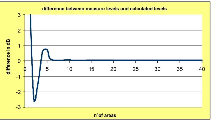
difference between measure levels and calculated levels
-3 -2 -1 0 1 2 3
0 5 10 15 20 25 30 35 40
n°of areas
[image:6.596.121.478.71.274.2]difference in dB
Figure 3. Difference in dB linked to n° of areas in the point A
This relationship between the measured value and the prevision difference cannot be noticed using the same method in the second sound level meter’s position. In this case, indeed, the trend of the difference decreases as the number of influence areas increase, and the floating previously observed cannot be seen. We can also stress that when we study the floating phenomenon of the differences, the prevision calculated in the point A of the figure (1), moves more rapidly to the real value.
The difference of the influence areas number we have to use in both cases, shows the shape called “pass by” where the car just moves in front of the receiver is more sensitive to the geometrical distances variation of the point sources considered, but the prevision moves at highest speed to real value. Therefore, the study of the number one sound level meter shape has to use a greater number of influence areas to obtain an acceptable prevision. Another important aspect to consider is the distance d0, the receiver’s distance from the car’s transit line,
and the test way’s length.
Through the experimental values we observe that increasing the distance d0 and maintaining
constant the way length, the prevision reaches a high degree of accuracy even with allowance of the influence areas number.
difference between measured levels and calculated levels
0 1 2 3 4 5 6 7
0 5 10 15 20 25 30 35 40
n° of areas
difference in dB
[image:6.596.133.462.528.745.2]It is now more evident than before that the increase or the decrease in the way’s length , brings respectively to an increase or decrease of the influence area’ s number necessary for the prevision.
CONCLUSION
Since many years noise is considered an important pollution element for people of industrialised countries. In this contest forecasting with a sufficient accuracy and evaluating the possible risk on human health is more and more necessary. Our work, starting from the state of art about the acoustic field’ s prevision method, links the ability in foretelling with sufficient accuracy the impact caused by the sound propagation together with the ability in evaluating the risks to which exposed people can incur. This method shows its potentialities in all those sectors where man is in deep touch with moving sound sources. We can thus state that many things can still be done in this field, by the help of a wide experimentation, to answer and solve in a satisfactory way the majority of the existing problems.
BIBLIOGRAPHY
[1] Kokowski P. Makarewicz R. “Interrupted Traffic Noise“; [2] ISO 6395;
[3] Bérengier M., Garai M, ‘’Propagazione del rumore da traffico veicolare’’
[4] CERTU, SETRA, LCPC, CSTB, ’’Bruit dees infrastructures routiéres. Methode de calcul incluant les effects météorologique’’.
[5] ISO 1996-1:1982 Acoustics - Description and measurement of environmental noise - Part 1: Basic quantities and procedures
[6] ISO 9613-2:1996: Acoustics - Attenuation of sound during propagation outdoors - General method of calculation.
[7] ISO 9613-1:1996 Acoustics-Attenuation of sound during propagation outdoors- Part 1: Calculation of the absorption of sound by the atmosphere.