COMPARATIVE ANALISIS OF SEVERAL ACOUSTIC IMPEDANCE MEASUREMENTS

COMPARATIVE ANALISIS OF SEVERAL ACOUSTIC IMPEDANCE MEASUREMENTS PACS:43.58.Bh

J. González Suárez1; M. Machimbarrena Gutiérrez1; A.Tarrero Fernández.2 ; T. Lorenzana

Lorenzana3; A. Moreno Arranz4

1

Dpto. de Física Aplicada de la E.T.S. de Arquitectura;

Avenida de Salamanca s/n. 47014 – Valladolid; Tel: +34 983 423446; Fax +34 983 423425

E-mail: juliog@opt.uva.es and mariao@opt.uva.es

2

Dpto. de Termodinámica y Física Aplicada de la E.U.P. C/ Francisco Mendizábal; Valladolid

Spain ana@sid.eup.uva.es

3

Dpto. de Física de la EUAT; Campus Zapateira; 15071- A Coruña; Spain; Tel: 981-167050

E-mail: lorenzan@udc.es

4.

Instituto de Acústica Torres Quevedo; Serrano 144; 28006- Madrid; Tel: 915618806

E-mail: iacma15@pinar2.csic.es

ABSTRACT

In this paper we present the experimental data for the acoustic impedance of different materials (typical ground and construction materials) according to different measurement techniques.

INTRODUCTION

When talking about ambient quality, especially in an urban environment, it is important to consider noise as an important factor. There are many different research groups working on sound propagation, and among all the parameters that affect this propagation, the ground impedance Z is an important one.

The purpose of our research is to evaluate, according to different techniques, the acoustic impedance of some of the ground materials commonly found in an urban environment, as well as some typical construction materials. We have measured over samples of earth with grass, concrete, two kinds of plaster (gypsum and thin construction plaster) and adobe. In some cases we have measured similar samples with different techniques, including the sound intensity technique.

MEASUREMENT METHODS

The different measurement methods used can be grouped in two types: direct and indirect methods.

The direct method group includes those methods that, with a specific measurement set up, are able to directly determine the impedance of the sample. Among these direct techniques we have used two specific ones: The first technique is based in the transfer function method and the impedance tube, the second technique uses the sound intensity method.

Indirect methods usually compare experimental sound attenuation with the sound attenuation predicted by an adequate propagation model.

diameter) and does not take into account the effect of a vast ground more or less homogeneous. In those cases where the samples can be adjusted to the experimental set-up without modifying their physical characteristics, then the measurement technique is really reliable and is preferred to any other technique. On the other hand, the intensity technique has the advantage that it is possible to measure under the normal using conditions of the material, that is, anywhere without any previous sample accommodation. The negative part is that the technique itself is not very easy to implement, the instruments are delicate and the range of validity of the measurements is frequently limited by the equipment and/or environment conditions.

All indirect methods have the advantage that they can consider a vast region and thus, the impedance results will be an average of the impedance of all the components of the wide region considered. These indirect methods are especially adequate for outdoor measurements. The inconvenient is that the existing sound propagation models are still being improved and require impedance models that, of course, are approximate. Another inconvenient is that the meteorological conditions may affect the measurement, and it is still under investigation how the meteorological parameters should be included in the models. Among the existing models some yield a better fit to the experimental data, depending on the factors that have been taken into account and on how accurate are the hypothesis used considering the real measurement conditions. [1], [2].

IMPEDANCE TUBE MEASUREMENTS

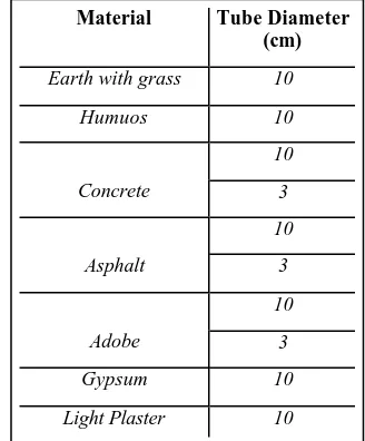
Since this method is commonly used and it is easy to find references about it in the existing literature, we will just show the results obtained for the different samples. As it can be seen in table I, for all cases we have tested 10 cm diameter samples and in some of them also 3 cm diameter samples were ested. This was done in order to have reliable results over a wider frequency reange. We have also tested different samples thicknesses in order to verify if the thickness is an important parameter. B&K 4206 impedance tube was used.

RESULTS

Grass and Humuos samples

The grass sample can be described as a grass surface with about 5 cm of earth below the grass. The humus sample was just a block of humus of about 5 cm too. Since both materials are not very rigid it was not possible to manufacture a 3 cm diameter sample and we measured only over a 10 cm diameter sample. As it can be seen in figure 1, both materials have rather low

relative impedance values, and a rather different behaviour. The grass has a relative impedance

minimum (twice ρ0c) near 340 Hz, which means that the absorption is maximum at this

frequency. Two maxima can be observed near 100 and 700 Hz (6 or 7 times ρ0c), the

absorption takes a minimum value at these frequencies. Above 700 Hz the absorption increases again. If we compare the grass results with the humus results, we can see that the humus relative impedance shows a continuous increasing tendency. That is, relative impedance varies from 15 relative units at 100 Hz to approximately 40 units in the higher frequency range.

0 2 4 6 8 10

100 340 580 820 1060 1300 1540 f[Hz] Impedancia magnitud

Fig. (1-a).- Relative impedance for grass sample.

0 20 40 60

100 400 700 1000 1300 1600

f[Hz] Z Impedancia magnitud

Fig. (1-b).- Relative impedance for humus sample.

Table I.- Materials and sample Material Tube Diameter

(cm)

Earth with grass 10

Humuos 10

10

Concrete 3

10

Asphalt 3

10

Adobe 3

Gypsum 10

Asphalt, Concrete and Adobe samples

Figure 2 (a), (b) y (c) show the relative impedance results for asphalt, concrete and adobe respectively. These materials can be easily found in an urban environment, and from an intuitive point of view at least asphalt and concrete can be considered as hard and highly reflecting. But if we look at the experimental curves we can observe that the behaviour of the asphalt sample is completely different form the behaviour of the concrete and adobe samples, both in shape and values. For the asphalt the maximum impedance appears near 700 Hz, reaching a relative value of about 60, whereas for concrete the maximum appears at much lower frequencies (around 350 Hz) and reaches an oscillating relative value of 300, much higher than for asphalt. The minimum values do not differ too much. As far as adobe results is concerned, the results are not so different to the concrete, except for the fact that the maximum is shifted to higher frequencies and the oscillations are more visible. There are also two other relative maxima, one at low frequencies and another one near 1500 Hz.

Gypsum and Light Plaster samples

Gypsum and light plaster are frequently found in traditional building construction, especially indoors. Figure 3 shows the experimental curves obtained for relative impedance. It is interesting to observe that the behaviour is rather different both in shape and values even though the materials are very

similar. The gypsum maximum appears near 700-900Hz, while for the light plaster there is a relative minimum around 600Hz and two maxima, one at low frequencies and the other one at medium to high frequencies, 1100 Hz.

INTENSITY TECHNIQUE MEASUREMENTS

Using a sound intensity probe allows to determine sound impedance of any material under real conditions and for any angle of incidence. This is an important advantage compared to the impedance tube technique. With the intensity probe it is possible to determine, simultaneously, the pressure and particle velocity in the region between two spaced microphones placed near the sample (large piece of ground, for example) under study. Once pressure and velocity are

determined, the impedance of the medium situated between both microphones Z1 can be

calculated just by dividing them. Assuming plane wave conditions, it is possible to determine the

impedance of the sample Z2 (where reflection has been produced) according to equation: Z2 =

[Z1-jρc tan(wd/c)]/(ρc-jZ1 tan(wd/c)], where d corresponds to the distance between the probe

center and the sample [4]. The main disadvantage of the intensity technique is the frequency validity range. The equipment used must have an excellent dynamic capability over a wide frequency range, which is not always possible.

Intensity measurements took place in a hemianecoic room, using B&K 2148 real time analyser, B&K 3545 intensity probe, B&K 3541 intensity calibrator and B&K 4224 sound source.

We have performed measurements over different samples such as: rock wool of different thickness, a foam and a cardboard. We have modified, successively, the source-sample

0 3 0 6 0 9 0 120 150

100 300 500 700 900 1 1 0 0 1 3 0 0 1 5 0 0 Hz Impedancia

Fig(3- a).- Relative impedance for gypsum sample.

0 80 160 240 320 400

100 340 580 820 1060 1300 1540 f[Hz] Impedancia magnitud

Fig(3-b).- Relative impedance for light plaster sample. Fig(2- b).- Relative impedance for

concrete sample 0

1 0 0 2 0 0 3 0 0 4 0 0

1 0 0 3 4 0 5 8 0 8 2 0 1 0 6 0 1 3 0 0 1 5 4 0 f[Hz] I m p e d a n c i a

0 15 30 45 60

1 0 0 3 4 0 5 8 0 8 2 0 1060 1300 1540 f[Hz] Impedancia magnitud

Fig(2- a).- Relative impedance for asphalt sample.

Fig(2-ca).- Relative impedance for adobe sample

0 100 200 300 400

distance (2 and 1.7 m), the size of the sample and the proble-sample distance. We have also measured with three different spacers in order to cover a wider frequency range. In this paper we include only the results for one of these sets of measurements made over rock wool.

In this case the rock wool sample had a density of 50 Kg/m3 and was 50 mm thick. The distance

between the probe center and the sample was the minimum possible, 50 mm, the spacer used was 12 mm and the source-sample distance was 2 meters. With this set up we can guarantee that the incident wave is approximately plane, the reliable frequency range is wide (100 – 5000 Hz) and the material sound absorption considerably high over all the frequency range.

Figure 4 shows the experimental results obtained for this sample with the intensity technique and with the impedance tube. As it can be seen, below 500 Hz (approximately) both curves diverge considerably, whereas above this frequency the results are almost identical for both measurement techniques. It is evident that the low frequency results must be wrong for one of the techniques, and it is easy to confirm that, in this case, it is the intensity technique that fails. The reason for this failure at low frequencies is the high reactivity of the field since at low frequencies the sample is not very absorbing and most of the sound energy is reflected.

We can conclude that, undoubtedly, the intensity technique has great advantages when used “in situ”, but it is necessary to guarantee the measurement conditions, by evaluating the field reactivity and comparing it to the equipment dynamic capability. Besides, it is important to find the right source-sample and probe-sample distances in order to ensure the right measurement conditions.

INDIRECT METHOD

Theoretical Background

Another way to determine ground impedance is using outdoor sound propagation models. The basic idea is to use a model to calculate the sound attenuation produced at a given point and then compare this predicted value with the experimental value obtained when measuring in that specific point. The model includes ground impedance as one of the multiple parameters that affect sound propagation. The impedance is introduced in the propagation

model as a function of frequency and of other parameters related to the ground, according to one of the different existing impedance models. There are impedance models considering 1, 2, or 4 parameters, as explained in references [1], [3]. We have selected Delany- Bazley’s impedance model among the different existing models due to its simplicity and to the good fit between the theoretical and experimental curves that was obtained with it. Figure 5 shows the relative source S and receiver R positions. The sound pressure at the receiver’s position is the

composition of the direct sound (trajectory r1) and the reflected sound (trajectory r2). In order to

avoid the source influence, the sound pressure level measured at the receiver’s position is divided by a measured reference value (R’ position) that is not affected by the reflection (not shown in figure 5). The attenuation in R referred to the reference value at R’, according to

Daigle’s model and considering r’1 and r’2 the direct and reflected trajectories for the reference

position, is given by:

φ φ

r1

r2

Fig. 5.-Typical geometrical representation for outdoor sound propagation.

R S

Modulo de la impedancia

0 3 6 9

50 125 315 800 2000 5000

f(Hz) z

tubo 12mm

Where Q is the spherical reflection coefficient

and is a function of the flow resistivity σ. From

the attenuation values we choose the σ value

that gives a better fit between the experimental values and the model. Then we calculate the ground impedance which, according to this model,

can be obtained by: Z2/Z1 = 1+9,08[f/σ]-0,75+j11,9[f/σ]-0,73(c.g.s.), where ground impedance is Z2

and the propagation medium impedance is Z1 (air, in general).

Measurements And Results

For all measurements we have used B&K 2144 analyser, B&K 4224 sound source, B&K 4129 microphones and B&K 2236 analyser as reference microphone.

We have used the indirect method over many different kinds of grounds commonly found not only in urban environments but also in the surroundings. From now on we will refer to these samples as: Weed land, Ploughed land, Sown field, Sand field, Earth field, Wet grass field and Concrete field.

Weed land

This land has a sandy but compact texture and was covered randomly with weedy vegetation of about 30 cm height and 1 to 2

mm of diameter. σ values for this kind of land

varies from 90 to 95 [g/(s.cm2)]. Figure 6

shows both the real and imaginary part of the corresponding impedance.

Ploughed land

The land had been ploughed but there was no vegetation in it. The surface was rather irregular with many “earth stones” within the land.

Sown field: Flat land sown with wheat of about 50 cm height.

Sand field: This was a large sand field.

Earth field: Hard compact earthfield, commonly used as young people’s football field.

Wet grass field: This was a reglamentary football field covered with a uniform grass.

The size of the field was 7.000 m2 and when the measurements were made it had just

been abundantly watered

Concrete field: In this case we used a big and empty parking lot with no obstacles within about 60 m around.

COMPARATIVE ANALYSIS OF

σ

σ

Table 2 shows the range of σ values that give a

best fit between the experimental and theoretical curves for six of the measured cases. From the results we can observe that the ploughed field

yields lower σ values so it is the one that gives

higher attenuation values. The values are very similar over all the frequency range (not shown in the table). The sown and sand fields have

slightly higher values for σ, but still rather low.

The earth and wet grass fields present medium σ values that do not vary very much at low

Attenuation

'

/

'

/

/

/

log

20

2 ' 1

'

2 1

10 _{1 2}

2 1

r

e

Q

r

e

r

e

Q

r

e

ikr t ikr

ikrr r ikr

+

+

=

SUELOS σ (c.g.s.)

Ploughed 10-20

Sown 50-70

Sand 100-140

Earth 400-500

Wet grass 700-850

Concrete 10000-100000

Table II.- Flow resistivity range values 0

3 6 9 12

1 0 0 2 5 0 6 3 0 1 6 0 0 H z4 0 0 0

Z R e a l I m a g

frequencies, but that take very small values between 630 Hz and 2000 Hz. Last but not least,

the concrete field yields very high σ values. The concrete is the material that attenuates the

least, although at low frequencies its behaviour is rather similar to the wet grass and the earth

fields. Again, attenuation is rather low between 630-1600 Hz. From the σ values obtained we

can conclude that the model is not very sensitive when σ values are very high. Notice that

almost any value between 10.000 and 100.000 produce a good fit between experimental results

and theoretical predictions. This is absolutely the opposite for low σ values, where a very small

change can misadjust the fit. Another important thing to point out about the model is that, in spite of the fact that it takes into account the potential geometric modifications, it does not consider the effect of other factor such as the meteorological ones, so the prediction for such set ups where the distances are big enough, may not be so reliable.

Since σ values have been obtained by comparing two curves (the experimental one and the one

given by the model) and “tuning” σ so that the

theoretical curve fits the experimental data, we include in figure 7 both curves for the case of the wet grass field. As it can be seen the theoretical model fits very well the experimental data, especially so at low frequencies. This is a good reason to believe in the reliability of the model for flow resistivity

measurements over wide samples. The σ values

obtained for wet grass is very different from what could be expected for dry grass, at least it is very different from what was obtained with the impedance tube for a grass sample.

CONCLUSIONS

We have studied different commonly found materials according to three different measurement techniques. We have found a fairly good agreement between all the techniques, although it is interesting to point out that:

• Impedance tube results show estrange oscillations due to irregularities in the samples

manufacture.

• Sound intensity results are not reliable at low frequencies if the sound field is highly

reactive and the equipment is limited by this high reactivity. A priori intensity measurements are adequate for “in situ” measurements.

• For wide extensions, the indirect method has turned out to be the most reliable and easy

to use method since there is no need to manufacture a sample and the measurement technique is very simple.

This research is part of a major project, AMB98-1029-C04-03, that has been developed with the financial support of the Spanish CICYT.

BIBLIOGRAPHY

[1] M.A. Price, K. Attemborough, “ Sound attenuation through trees: Measurements and models”, J. Acoust. Soc. Am. (1988) 84(5)

[2] Embleton, T. F. W.; Piercy, J. E.; Daigle, G. A. “Effective flow resistivity of ground surfaces determined by acoustical measurements”. J.A.S.A. 74, (4); October 1983.

[3] Delany, M. E.; Bazley, E. N. “Acoustical properties of fibrous absorbent materials”. Applied Acoustics, 3, 1970.

[4] Allard, J. F., Aknine, A., “Acoustic Impedance Measurements with a Sound Intensity Meter”. Applied Acoustics 18, 69-75 (1985).

[5] J. González; M. Machimbarrena; A. Pérez; T. Lorenzana. “Medida directa de la impedancia

acústica de distintos materiales”. (Tecniacústica´2001). Octubre 2001. La Rioja, España.

[6] Embleton,” Resisyivity of ground surfaces”, J.Acoust. Soc. Am. Vol 74, Nº 4, Octubre (1983) [7] Embleton, T. F. W.; Piercy, J. E.; Olson, N. “Outdoor sound propagation over ground of finite impedance”. J.A.S.A. Vol 59; No 2; February 1976.

Fig.7.- Sound attenuation for wet grass. Theoretical (σ=800 )and experimental .

C é s p e d H ú m e d o

- 4 0 - 3 0 - 2 0 - 1 0 0

1 0 0 2 5 0 6 3 0 1 , 6 k _{H z} 4 k

Atenuación (dB)