NUMERICAL MODELING OF THE NONLINEAR PROPAGATION OF TRANSIENT ACOUSTIC SIGNALS

(1)

NUMERICAL MODELING OF THE NONLINEAR PROPAGATION OF

TRANSIENT ACOUSTIC SIGNALS

PACS REFERENCE: 43.25.Cb

Campos-Pozuelo C.1

; Vanhille C.2

1

Instituto de Acustica

Serrano, 144, 28006 Madrid, Spain

Tel: +34.91.561.88.06; Fax: +34.91.411.76.51; E-mail: ccampos@ia.cetef.csic.es

2

ESCET. Universidad Rey Juan Carlos. Tulipán, s/n. 28933 Móstoles, Madrid. Spain

Tel: +34.91.664.74.82; Fax: +34.91.664.74.90; E-mail: c.vanhille@escet.urjc.es

ABSTRACT. A numerical study of high-amplitude transient signals propagating in an absorbing, homogeneous fluid is presented. The work is motivated in many applications where high intensity waves, which can not be described by linear laws, are involved (biomedical research, high power ultrasonics, etc.). Differential equations are written in lagrangian coordinates, and the full nonlinear equation is solved by means of a finite difference algorithm. Calculations are performed exclusively in the time domain, giving all the harmonic amplitudes by only one resolution step, and allowing the analysis of the evolution of the waveform for any original signal: gaussian, rectangular pulses, periodic excitation, etc. Numerical results are presented for waveform distortion and shock formation for plane transient and harmonic waves. Spatial and initial pulse shape dependences are specially analysed.

INTRODUCTION

This paper deals with a numerical study of high-amplitude acoustic signals propagating in an absorbing, homogeneous fluid. Many applications exist where high intensity waves, which can not be described by linear laws, are needed. In particular, the development of medical ultrasound as a therapy tool (hyperthermy, lithotripsy, etc.) involves high amplitudes and, thus, nonlinear propagation. In the other hand we observe an increase in the amplitudes of the ultrasonic fields applied in diagnostic in order to have greater penetration and greater resolution [1]. The theory accompanying this development can not be made anymore under the assumption of linear propagation. In this framework, the purpose was to develop a numerical method for studying the nonlinear propagation of plane waves by using the full nonlinear equation derived in lagrangian coordinates. Some authors have used eulerian coordinates and the “retarded time” variable associated with the propagation in the

+

x

direction:

τ

=

t

−

x

c

₀, which allows them to reduce by one the order of the differential equation for wave motion [1,2]. In this paper we solve the full nonlinear differential equation written in lagragian coordinates by using natural spatial and time coordinates. This implies the need of imposing a non-reflecting boundary condition. The formulation is written in the time domain, allowing the analysis of the evolution of the waveform for any original signal: periodic excitation, gaussian, rectangular pulses, etc. In addition, all the harmonic components are obtained by only one resolution step, with the consequent save in computation time.

(2)

I. FUNDAMENTAL EQUATIONS

Nonlinear waves propagating in a homogeneous thermoviscous fluid are studied. The Tait-Kirkwood equation of state for isentropic fluids has been considered [1]. The one-dimensional full nonlinear wave equation written in lagrangian coordinates is considered [3]:

(

)

ρ

∂

χ

π

∂

ρν

∂

∂ ∂

χ 0

2

2 0 1

2

2 0

3 2

1

1 u

t

p

u

x

u

x

b

u

t x

=

+









+

+ , (1)

where p0 is the ambient pressure, ρ0 the initial state density, π and χare characteristic constants

of the fluid,

u

is the displacement, v is the kinematic shear viscosity, and b is the so-called viscosity number. t and x are, respectively, the time and one-dimensional spatial coordinates. No approximations have been made about the acoustic Mach number value or about the attenuation parameter, i.e., the only limitations on pressure amplitude in the model are those derived from the isentropic approximation [3]. However, since we consider the propagation of a (transient) wave within an unbounded domain, even in the case of very high acoustic Mach number, the isentropic property of the fluid can not be questioned.

Boundary conditions

We consider progressive plane waves and a source placed at

x

=

0

. Then, the following boundary conditions are written:

( )

0

0 0,

,

, ,

x

u

t

f

t

u

x

L

c

L t

x

t

=

∂

=

= −

∂

(2.a)

(2.b)

where

c

₀ is the small-amplitudes value of the sound speed, L is the length of the domain considered in calculations. The “quasilinear” non-reflecting condition (2.b) will be tested by comparing the numerical results with analytical results obtained for an harmonic wave.

f

(

t

)

is the source function, i.e., the excitation of the medium defined as a function of time. The method supports any source function. In this article some numerical experiments are made by considering different dependencies for

f

(

t

)

: a continues wave and two gaussian pulses of different length.

The fluid is assumed to be initially at complete rest: particle displacement and velocity are null at t

= 0. The following initial conditions are then employed:

( )









≠

∀

=

0

0 ,

0

0 ,

0 x

t

x

u

x

u

t

∂

. (3)

Heating

It is well known that the absorption of sound leads to heat generation in the acoustic medium. Moreover, temperature is a very important parameter in applications, especially in medical applications. When dealing with very high amplitude waves the nonlinear attenuation is completely dominant (see Figure 1) and then the heating predicted by a linear theory is not correct anymore and it has to be calculated in the new nonlinear framework. We calculate the heating rate and the temperature increase by using the isentropic hypotheses [3] and the Fourier’s law,

0.0E+0 1.0E-1 2.0E-1 3.0E-1 4.0E-1

S patial coor diante (m)

0.0E+0 4.0E+3 8.0E+3 1.2E+4 1.6E+4

P

re

s

u

re

(

P

a

)

L inear c alculat ions

[image:2.596.92.299.301.477.2]

N onlinear calc ulat ions

Fig. 1. Comparison of the amplitude evolution at the fundamental frequency for a strongly

(3)

0

3

2

2 2

=









∂













₊

+

x

t

u

x

B

∂

µ

∂

θ

∂

κ

, (4)

x

q

∂

∂θ

κ

−

=

, (5)

where

q

is the heat-flux,

θ

the absolute temperature,

κ

is the coefficient of thermal conductivity, and

µ

and

µ

_B are the viscosity and bulk viscosity. No-additional hypotheses about the acoustic Mach number has been made. These equations are solved by using a conventional finite differences algorithm [4].

II. NUMERICAL FORMULATION

In this section the numerical formulation developed for solving the acoustical problem is described. It is based on the finite-difference method [5] and has been included in the numerical code Snow-ac [3,8].

The numerical scheme is created by considering two dimensionless independent variables: X=x/λ and

T=ωt, where λ is the wavelength of the signal and ω is its angular frequency, and an uniform discretization of the X-T

space. The differential equations of the previous section are numerically treated as in reference [3,6]. Displacements are evaluated at every point of the discretized space. The method is implicit and conditionally convergent [3,6]. Boundary conditions (2) are taken into account at each time-step. A notable feature of the method is the linear structure of the system of equations obtained at each time-step for solving the nonlinear problem.

The mechanical perturbations of the wave reach the wavelength number i at the period number i, and thus many values of the displacement are null. This phenomenon is taken into account in the algorithm. These null values are not evaluated. This fact generates an important saving of operations, storage and CPU time. For this purpose computations are first led on the perturbated zone during the first group of periods only, by considering the initial conditions. The number of periods of the group depends on the kind of pulsed excitation. The second phase computes the values of the displacement on the perturbed zone during the second group of periods, by considering a continuity condition with the first part. And as so on up to the last group of periods of the problem.

At each time-step of the j-th period the system of equations is solved by means of an economic and fast method based on a LU decomposition valid for the whole j-th period [7].

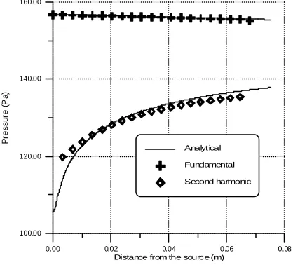
0.00 0.02 0.04 0.06 0.08

Distance from the source (m) 100.00

120.00 140.00 160.00

P

re

s

u

re

(

P

a

)

Analytical

Fundamental

[image:3.596.104.313.185.374.2]

Second harmonic

Fig. 2. Comparison with analytic results for

kHz

20 =

f

, 5 periods, 5 wavelengths, and

1

m

06 .

2

−

=

α

0.00E+0 2.00E- 6 4.00E- 6 6.00E-6 8.00E-6 Tim e ( s)

-8.00E-1 -4.00E-1 0.00E+0 4.00E-1 8.00E-1 1.20E+0

P

is

to

n

d

is

p

la

c

em

en

t

(N

o

rm

al

iz

ed

u

n

its

)

G aus s ian pu lse

S hort puls e

(4)

Pressure and heating rate are calculated from the displacement values by means of classic finite-difference schemes.

III. VALIDATION AND RESULTS

A validation of the numerical method is presented by comparing with analytical results referred to a quasi-linear case. The analytical model is based in a perturbation technique in the frequency domain. We assume a solution consisting in the addition of two terms in the form

u

= +

u

_l

u

₂,

2

0

p

−

=

_l

+

and with

u

₂

<<

u

_l and

p

₂

<<

p

_l, where

u

_l

( )

p

_l represents the first-order solution of Eq. (1) and

u

₂

( )

p

₂ the second-order correction. The additional assumption of small attenuation is made and dissipation is taken into account by using a complex wave number. With these approximations, the following analytical solution is obtained:

( )

( t kx)

j l

kx t j l

ke

c

j

p

e

u

− −

=

ω ω

ρ

2 0 0 0

( )

(

)

j( t kx)

kx t j

e

kx

j

u

k

c

p

xe

u

k

u

− −

+

−

=

+

−

=

ω ω

γ

ρ

γ

2 2

0 2 2

0 0 2

2 2 0 2 2

2

1

8

1

8

1

(6)

where

k

=

k

₀

−

j

α

, and

0 0

c

k

=

ω

. In Figure 2 analytical and numerical results are compared. A

harmonic source of amplitude

u

₀

=

25 µ

m

is considered at the frequency

f

=

20000

Hz

.

m/s

340

0

=

c

,

γ

=

1 .

4

and

ρ

₀

=

1 .

29 kg/m

3. We consider

α

=

2 .

06 m

−1.

h

=

0 .

01

is employed. The numerical sound pressure distribution of the first and second harmonics at the last instant of the study is shown to coincide with the analytical one. The harmonic decomposition of the numerical signal is obtained by means of a FFT. These good results validate the numerical method presented.

Some results are now presented referring to the propagation of transient signals. The source

function is written as

f

( )

t

u

e

[xb(t t )]

_cos

( )

ω

t

2 0

0

− −

=

. We have chosen two short signals: a very

short pulse

(

x

_B

=

5 ×

10

6

)

and a gaussian pulse

(

x

_B

=

10

6

)

. The evolutions of the waveshapes and shock formation are studied and the importance of the initial waveshape analysed. In all cases we have considered a fluid with acoustic properties similar to tissues of the body (with the exceptions of lung, bone, and fat):

c

₀

=

1500

m/s

,

γ

=

6 .

2

and

ρ

₀

=

1000

kg/m

3,

1

m

11

−

=

α

[1]. We consider a frequency of 1 MHz, quite usual in medical applications. In Figure 3 we see the considered displacement at the piston in normalized units. The displacement amplitude at the piston is

u

₀

=

1 .

5 µ

m

, which means an initial pressure amplitude of the order of 15 MPa, quite typical in medical applications, both diagnostics (in focalized region) and therapy. In Figure 4 we show the evolution of the waveshape for the two considered cases. We observe that the strong harmonic distortion occurs at the first wavelengths from the source in both cases. When distance to the source increases, the central frequency of the short gaussian pulse decreases. At 7.2 cm from the source the pulse has an amplitude of the order of 27% of its initial value and its frequency is about three times less than the original; no much harmonic distortion affects this state of the pulse. Thus, for this type of excitation signal, the main effect involved is the nonlinear attenuation associated with the harmonic distortion in a nonlinear medium with a dispersion relation of the type ω2

(5)

REFERENCES

1. Nonlinear Acoustics, ed. By Hamilton MH and Blackstock DT. Academic Press: New York,
1998
2. D. T. Blackstock, “Propagation of plane sound waves of finite amplitude in nondissipative fluids”, J. Acoust. Soc. Am., 34, 9-30 (1962)
3. Vanhille C and Campos-Pozuelo C. “Numerical model for nonlinear standing acoustic waves and weak shocks in thermoviscous fluids”, J. Acoust. Soc. Am. 2001; 109: 2660-2667
4. Vanhille C and Campos-Pozuelo C., “Three computational models for quasi-standing nonlinear acoustic waves”, submitted for publication to Journal of Computational Acoustics
5. Smith GD. Numerical solution of partial differential equations, Finite Difference Methods. Clarendon Press: Oxford, 1985.
6. Vanhille C and Campos-Pozuelo C. “A High-Order Finite-Difference Algorithm for the Analysis of Standing acoustic Waves of Finite but Moderate Amplitude”, J. Comput. Phys. 2000; 165: 334-353.
7. Vanhille C and Campos-Pozuelo C. “Étude numérique d’ondes ultrasonores progressives d’amplitude finie”, Actes du 6ème Congrès Français d’Acoustique, (2002).
0. 0E +0 2. 0E- 2 4. 0E-2 6 .0 E-2 8. 0E- 2
Spatial coordinate (m)
0.0 0.2 0.4 0.6 0.8 1.0
P
re
s
u
(
N
o
rm
a
liz
e
d
v
lu
) Short pulse
Gaussian pulse Fundamental
Demodulation frequency
[image:6.596.98.321.170.388.2]