Characterization of inequality changes through microeconometric
decompositions.
The case of Greater Buenos Aires
Leonardo Gasparini, Mariana Marchionni y Walter Sosa Escudero
C
haracterization of inequality changes
through microeconometric decompositions
The case of Greater Buenos Aires
*Leonardo Gasparini Mariana Marchionni Walter Sosa Escudero
Universidad Nacional de La Plata **
This version: July 1, 2000
Abstract
We apply a variant of the microeconometric decomposition methodology proposed in Bourguignon et al. (1998) to assess the relevance of various factors that affected inequality in the period 1986-1998 in the Greater Buenos Aires area. The results of the paper suggest that the small change in inequality between 1986 and 1992 was the result of mild forces that compensated each other. In contrast, between 1992 and 1998 nearly all factors had some role in increasing inequality to unprecedented levels. The increase in the returns to education, changes in endowments of unobservable factors and their remunerations, and the fall in hours of work by low-income people are particularly important to explain the growth in inequality in the nineties. In contrast, although Argentina witnessed dramatic changes in the gender wage gap, the unemployment rate and the educational structure, these factors appear to have had only a mild effect on the household income distribution.
Keywords: inequality, decomposition, education, earnings, unemployment, Argentina.
JEL Classification: C15, D31, I21, J23, J31
*
This article is part of a project on income distribution financed by Convenio Ministerio de Economía de la Provincia de Buenos Aires - Facultad de Ciencias Económicas de la Universidad Nacional de La Plata. We thank the financial support of these institutions. We also thank Verónica Fossati and Alvaro Mezza for efficient research assistance. All opinions and remaining errors are responsibility of the authors.
**
1. Introduction
The main economic variables have widely oscillated in the last two decades in Argentina in association with deep macroeconomic and structural transformations. After reaching a peak of 172% monthly in 1989, the inflation rate decreased to less than 1% yearly in a few years; GDP drastically fell at the end of the eighties and then grew at unprecedented rates in the first half of the nineties; unemployment rose steadily from around 5% to 14% in a short period of time. Income inequality was not an exception in this turbulent period. The Gini coefficient increased from 41.9 to 46.7 between 1986 and 1989, fell to 40.0 towards 1991, and rose steadily in the following 7 years, reaching a record level of 47.4 in 1998.1 It is difficult to find in recent economic history periods with such marked changes in inequality, in Argentina as well as in the rest of the world.
The reasons of these changes in inequality are varied and complex. The main aim of this paper is to assess the relevance of some forces that are believed to have affected income inequality in the Greater Buenos Aires area between 1986 and 1998. More specifically, the microeconometric decomposition methodology proposed by Bourguignon, Ferreira and Lustig (1998) is used to measure the relevance of various factors that appear to have driven changes in inequality. In particular, this methodology is used to identify to what extent changes in the returns to education and experience, in endowments of unobservable factors (such as individual’s innate ability) and their returns, in the wage gap between men and women, in labor market participation and hours of work, and in the educational structure of the population contribute to explain the observed changes in income distribution.
The results of the paper suggest that the observed similarity between the inequality indexes of 1986 and 1992 is in fact the consequence of mild forces that operated in different directions, but compensated each other in the aggregate. On the contrary, between 1992 and 1998 nearly all the determinants under study have contributed to increase inequality. The increase in the returns to education, a higher dispersion in the endowments and/or the returns to unobservable factors and the dramatic fall in the hours of work of less-skilled low-income people appear to be the dominating forces. Perhaps surprisingly, neither the narrowing of the gender wage gap nor the increase in average education of the population were significant equalizing factors. Also, the dramatic jump in unemployment in the nineties does not appear to have had a very significant direct effect on household income inequality.
The rest of the paper is organized as follows. Section 2 shows the basic facts and discusses some factors that might have affected inequality in the last two decades. Section 3 presents the decomposition methodology implemented to assess the relevance of those factors, while section 4 explains the estimation strategy. The main results of the analysis are presented in section 5. The paper concludes with some brief final comments in section 6.
1
2. Income inequality: basic facts and sources of changes
Income inequality in Argentina has fluctuated considerably around an increasing trend initiated in the mid-seventies. Figure 2.1 shows the Gini coefficient of equivalent household income between 1985 and 1998 in the Greater Buenos Aires area.2,3
After a substantial increase in the late eighties, inequality plunged in the first two years of the nineties. A new stage of rising inequality started in 1992 and has not stopped yet. The Greater Buenos Aires has never experienced the level of income inequality reached in 1998, at least since reliable household data sets are available.4
For simplicity this study is focused on three years of relative macroeconomic stability separated by equal intervals: 1986, 1992 and 1998. Also, we restrict the analysis to labor income mainly for two reasons.5 (i) The Permanent Household Survey (EPH) has various deficiencies in
capturing capital income, and (ii) modeling capital income and retirement payments is not an easy task, especially considering the scarce information contained in the EPH. We also ignore those households whose heads or spouses are older than 65 or receive retirement payments. Summing up, we concentrate on the distribution of individual labor income and on the distribution of equivalent household labor income in 1986, 1992 and 1998 in the Greater Buenos Aires area.
Table 2.1 shows the basic facts to be characterized in the paper: inequality in individual labor income and in equivalent household labor income, as measured by the Gini, did not change very much between 1986 and 1992; on the contrary, both measures rose dramatically in the next six years.6
Gasparini and Sosa Escudero (1999) use bootstrap methods to show that it is possible to reject the null hypothesis that the Gini coefficients of 1986 and 1998 are equal. While the same is true for 1992 and 1998, one cannot reject the null hypothesis that the Gini coefficients of 1986 and 1992 are equal.
A countless number of factors may have caused the changes in inequality documented in table 2.1. We will concentrate in seven of them: (i) returns to education, (ii) the gender wage gap, 7 (iii)
returns to experience, (iv) the dispersion in the endowment of unobservable factors and their returns, (v) hours of work, (vi) labor market participation, and (vii) the education of the working-able population.
2.1. Returns to education
2
Following Buhmann et al. (1988) the equivalent household income is obtained by dividing household income by the number of equivalent adults (taken from the local National Institute of Statistics and Census (INDEC)) raised to .8, a parameter which implies mild household economies of scale.
3
The use of other indices do not change the main conclusions driven from the graph. See Gasparini and Sosa Escudero (1999).
4
These broad trends are also reported by other authors. See Altimir, Beccaria and González Rozada (2000), Gasparini (1999), Lee (2000) and Llach and Montoya (1999).
5
Labor income comprises wage earnings and self-employed earnings.
6
All households with valid incomes (including those with no income) are considered in the equivalent household labor income statistics. Ignoring those with zero income does not alter the main results (see our companion paper, Gasparini, Marchionni and Sosa Escudero (1999)). As usual, only workers with positive earnings are included in the individual labor income statistics. Results in table 2.1 are robust to changes in inequality indices (see our companion paper).
7
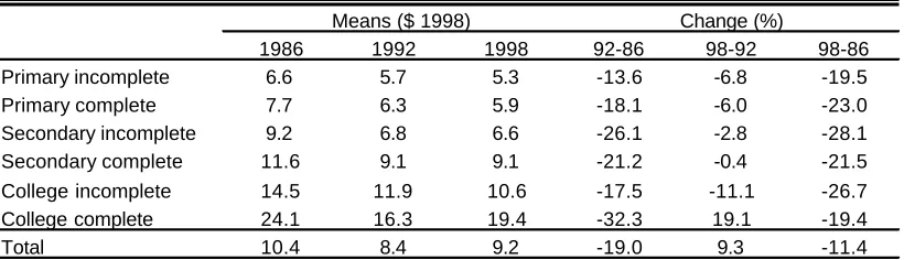
An increase in the returns to education implies a widening of the wage gap between high and low-educated workers, which in turn would imply a more unequal distribution of individual earnings and probably a more unequal distribution of household income. Table 2.2 shows hourly earnings in real pesos for workers between 14 and 65 with valid and complete answers. The average wage fell 19% between 1986 and 1992 and increased 9.3% in the next six years. Changes were not uniform among educational groups. While in the first period of the analysis the most dramatic drop in hourly earnings was for the college complete group, that group enjoyed the greatest increase in wages during period 1992-1998. Table 2.2 is a first piece of evidence that changes in relative wages among schooling groups implied a decrease in earnings inequality between 1986 and 1992 and an increase thereafter.
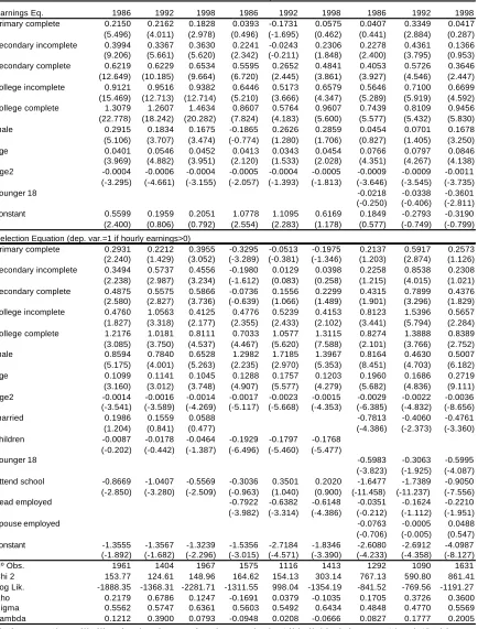
Table 2.3 shows the results of Mincerian log hourly earnings functions estimated using the Heckman procedure to correct for sample selection. The first three columns refer to household heads (mostly men) and the rest to spouses (nearly all women) and other members of the family (roughly half men and half women), respectively. Since the EPH does not record years of education we include dummies that capture the maximum educational level achieved. The omitted category is primary incomplete. A gender dummy, age and age squared and a dummy for youths less than 18 years old (only relevant for other members) are also included in the regression. In addition to those variables, the selection equation includes marital status, number of children and a dummy that takes the value 1 when the individual attends school. Following Bourguignon et al. (1999) it is assumed that labor market participation choices are made within the household in a sequential fashion. Spouses take the heads labor market status into consideration to decide whether to enter the labor market or not. Other members of the family consider both the head and the spouse labor market status.
The coefficients of most educational levels are positive, significant and increasing with the educational level, that is, the returns to education are always positive.8
For family heads in 1998, an individual with complete elementary school had a hourly wage 18% greater than an individual with incomplete elementary education, keeping all other factors constant. The same figure for incomplete high school, complete high school, incomplete college and complete college education is 36%, 65%, 94% and 146%, respectively, all with respect to the base category. It is interesting to observe that in many cases returns to education are increasing, that is, the hourly wage gap between educational levels increases with education.9
For the case of family heads in 1998 the difference in wages between an individual with complete elementary school and one with incomplete high school is 18%, whereas the difference between this level and complete high school is 29%. The greatest jump is between incomplete and complete college (52%).
Figure 2.2 shows the predicted hourly earnings for all different educational levels. The first panel refers to male heads and the second to other male members, both with age kept constant at 40.
8
We refer as “returns to education” the change in hourly wages due to a change in the educational level (and not in years of education). It takes around 7 years to complete the primary school, 5 or 6 additional years to complete high-school and around 5 years to complete college.
9
The wage-education profiles for family heads have a marked positive slope and are almost parallel everywhere, except for the substantial increase in the slope between 1992 and 1998 in the highest educational levels. This certainly contributes to increase earnings inequality among household heads with different educational levels. For male other-members the wage-education profile became flatter between 1986 and 1992 and substantially more steeper and convex in the next 6 years. The latter movement could imply a dramatic widening of the earnings gap by educational level.
Figure 2.3 shows the profiles for 40 years old females. As in the case of men the wage-education profiles show a decreasing slope between 1986 and 1992, and an opposite movement between 1992 and 1998. The increase in convexity in 1998 is particularly evident for other members. Summarizing, there is evidence of a positive relationship between hourly earnings and education which induces differences in incomes among individuals with different education. According to the evidence presented these differences have shrunk between 1986 and 1992, and have substantially increased in the next 6 years. The wage-education profile has become steeper and more convex. Although this phenomenon seems widespread across groups, it appears to be particularly relevant for the group of other members of the household.
2.2. Gender wage gap
Table 2.4 presents mean hourly wages by gender. Wages were higher for males in every year. In 1986 males’ hourly wages were on average 16% higher than females’. The gender gap narrowed to 3% in 1998.10
A conditional analysis also shows a shrinking gap for household heads. From table 2.3 the coefficient for the male dummy is always positive and significant, but clearly decreasing over time. Surprisingly, the time pattern is the opposite for other members. However, since the number of working individuals in this group is much less than in the household heads group, the global conclusion of a narrowing gender wage gap holds. This shrinking gap has undoubtedly been an equalizing factor on the individual earnings distribution. The effect of that phenomenon on the equivalent household labor income distribution will basically depend on the position of working women in that distribution. Section 5 has more on that.
2.3 Returns to experience (age)
Age is used in this paper as a proxy for experience in the labor market. Table 2.5 shows average hourly earnings for different age groups. In general the wage-age profile has an inverted U shape. Between 1986 and 1992 hourly wages fell, most significantly for older individuals, who are also the richest ones in terms of hourly wages. The youngest workers, who are the worst-paid, were the least damaged by the generalized wage drop. In principle this would imply an equalizing effect on the earnings distribution. However, these two groups together represent less than 9% of the total working population. For the rest of that population changes in hourly earnings did not follow a definite pattern.
10
Between 1992 and 1998 hourly wages grew for workers older than 30 and fell for the rest, which would imply an unequalizing effect. However, by far the most-favored group by the wage increase was the 50-59. This implies an equalizing force since the average wage of this group in 1992 was relatively low.
So far the probable effect of changes in returns to experience on inequality has not been clear. The coefficients of age and age squared in the log hourly earnings equation of table 2.3 provide more elements to the analysis. Particularly interesting is the substantial increase in the coefficient of age for household heads between 1986 and 1992 and the fall in that coefficient for spouses. Keeping all other things constant, this change would imply a widening of the wage gap between heads and spouses driven by differential changes in the returns to experience. Since heads’ wages are substantially higher than spouses’, that change in returns would be an unequalizing factor. An exactly opposite change in coefficients took place between 1992 and 1998, leading to an equalizing effect.
Summing up, there are some reasons to believe that changes in the returns to experience have led to higher inequality and some reasons to believe the opposite. The analysis of section 5 will help us to assess the quantitative relevance of each argument.
2.4. Unobservables
Earnings equations allow the estimation of returns to observable factors like education and experience. The error term is usually interpreted as capturing the joint effect of the endowment of non-observable factors (like individual ability) and its market value on earnings. In general terms, the variance of this error term captures the contribution of dispersion in unobservable factors to general inequality. Table 2.3 reports the standard deviation of the error terms of each log hourly earnings equation (labeled as “sigma”). For instance, for household heads the standard deviation took a value of .55 in 1986, .57 in 1992, and .64 in 1998. The substantial increase between 1992 and 1998 is also present in the spouses and other members equations. According to these results the effect of changes in unobservable factors would have been mildly unequalizing between 1986 and 1992, and substantially unequalizing in the next 6 years period.
2.5. Hours of work
The period under analysis has witnessed a slight fall in weekly hours of work: 1 hour between 1986 and 1992 and less than half an hour in the next six years. That fall was not uniform across workers. Table 2.6 classifies workers by educational level and records the average hours of work of each group. While there is not a clear pattern of changes between 1986 and 1992, the nineties have witnessed a dramatic fall in hours of work by low-education workers. This change would have a non negligible unequalizing effect in the individual earnings distribution.
in hours for the rest of the educational groups were only marginal. The fall in hours of work for low-educated female spouses was also greater than for the rest of the groups.
2.6. Labor market participation
Household income inequality can change not only after changes in hours of work but also as a result of changes in labor market participation. This is a particularly interesting point to study in the Argentinean case, since the dramatic jump in the unemployment rate in the nineties is thought to be the main responsible of the increase in inequality by many analysts.
In table 2.8 individuals are grouped according to whether they are employed, unemployed or inactive. The percentage of unemployed individuals rose from 2.3% in 1986 to 6.5% in 1998.11
The major increase took place between 1992 and 1998. However, notice that the increase in unemployment was accompanied by a decrease in inactivity of roughly the same magnitude. Despite the jump in the unemployment rate, the proportion of working-able people with zero income remained roughly unchanged between 1986 and 1998. Notice that for inequality measures it is irrelevant whether the individual has zero income because she is unemployed or because she is not looking for a job. Hence, aggregate changes in labor market participation might not have played a significant role on inequality changes.
Table 2.8 suggests three different stories in the labor market for heads, spouses and other members. Some household heads lost or quit their jobs, especially in the last 6 years, becoming either unemployed or out of the labor force. In contrast many of the spouses left their homes in search of a job: most of them found one between 1986 and 1992, but some of them did not in the 1992-1998 period. The other members of the family were less lucky: nearly all of them who started to look for a job became unemployed (or displaced another individual in that category).
Table 2.9 presents the proportion of adults employed, unemployed and inactive by educational group. Neither changes in unemployment rate nor changes in the proportion of people with zero income have clear patterns across educational groups. In principle, there are no clear signs that the strong increase in unemployment, especially during 1992-1998, has translated into a disproportionately increase in adults with no income in the low-education low-income group. The results of the selection equations in table 2.3 are in line with this conclusion.
Summing up, while differential changes in hours of work seem to have had a significant unequalizing effect on the earnings distribution, and hence probably on the household labor income distribution, the effect of changes in participation rates is not clear. It is likely that despite the enormous increase in unemployment rates in the Greater Buenos Aires area, changes in participation rates had had a negligible effect on inequality.
2.7. Education
11
In Argentina, as in many developing countries, substantial changes in the educational composition of the population have been taking place in the last decades. Table 2.10 presents the proportion of individuals between 14 and 65 years old by educational level. Between 1986 and 1998 there was a strong contraction in the proportion of youths and adults with elementary education (both complete or incomplete), which are groups with relatively low hourly wages. Simultaneously, between these years the proportion of individuals in all other educational groups increased, particularly in the college (incomplete or complete) group.
Education is usually viewed as an equalizing force. The traditional argument points out that income disparities in one generation can be reduced in the next one if poor children have access to more and better education, so that the educational gap with rich-families’ children narrows down. But following Kuznets (1955) one can tell a different story if the high-educated rich are a minority and only some poor children manage to make it all the way up to the highest educational (and income) levels. In that case it is likely that inequality grows as the average education of the population increases, at least until the high education group is relatively large. With multiple educational levels a similar unequalizing outcome emerges if there is a net outflow from the lowest educational levels and a similar net inflow to the highest levels, with minor changes in the intermediate levels. Changes in the educational structure from 1992 to 1998 have more or less taken that form, which feeds the presumption of an unequalizing education effect. Ten percent of the adults population left the primary education group, while six percent entered the college group. Changes from 1986 to 1992 are less clear, since five percent left the primary education group but less than half of that fraction entered the college group.
So far we have analyzed several factors that might have affected inequality. Although we have offered some evidence to argue about each effect we still do not have a consistent framework where to confirm the sign of each effect and where to assess its quantitative relevance. Were changes in the returns to education really an unequalizing force? Were they really a significant force? What about the gender, the employment or the education effects? The next section presents a framework to tackle these questions.
3. The methodology
To assess the relevance of the various factors discussed in the previous section on income inequality changes, we adapt the microeconometric decomposition methodology first proposed by Bourguignon, Ferreira and Lustig (1998) to our case.12
Let Yit be individual’s i labor income at time t, which can be written as a function F of the
vector Xitof individual observable characteristics affecting wages and employment, the vector εit of
unobservable characteristics, the vector βtof parameters that determine market hourly wages and the
12
Variants of the basic methodology have been applied in Altimir, Beccaria and González Rozada (2000),
vector λtof parameters that affect employment outcomes (participation and hours of work).
(1) Yit = F(Xit,εit,βt,λt) i=1,...,N
The distribution of individual labor income can be represented as
(2) Dt =
{
Y1t,...,YNt}
We can simulate individual labor incomes by changing one or some arguments in equation (1). For instance, the following expression represents labor income that individual’s i would have earned in time t if the parameters determining wages had been those of time t’, keeping all other things constant.
(3) Yit(βt')=F X( it,ε β λit, t', t) i=1,...,N
More generally, we can define Yit(kt’) where k is any set of arguments in (1). Hence, the simulated
distribution will be
(4) D kt( t')=
{
Y1t(kt'),...,YNt(kt')}
The contribution to the overall change in the distribution of a change in k between t and t‘, holding all else constant, can be obtained by comparing (2) and (4). Although we can make the comparisons in terms of the whole distributions, in this paper we compare inequality indices I(D). Therefore, the effect of a change in argument k is defined by13
(5) E kt( t')≡ I D k( t( t'))−I D( t)
As it was discussed in the previous section this paper is devoted to discuss the following effects: (i) Returns to education (k = βed): it measures the effect of changes in the parameters that relate
education to hourly wages (βed
) on inequality.
(ii) Gender wagegap (k = βg): the same as (i) but with gender.
(iii) Returns to experience (k = βex): the same as (i) but with experience.
(iv) Returns to unobservable factors (k=εw): it measures the effect of changes in the unobservable factors and their remunerations affecting hourly wages (εw
) on inequality.
(v) Employment (k = λ): it measures the effect of changes in the parameters that determine participation and hours of work (λ) on inequality.
13
In the empirical implementation we compute the labor income distribution only for those individuals such that
(vi) Education (k = Xed): it measures the effect of changes in the educational levels of the population (Xed) on inequality.
The previous discussion refers to the distribution of individual earnings. However, it is more relevant from a social point of view to study the distribution of household income since a person’s utility usually depends not on her own earnings but on her household income and demographic composition. Following Buhmann et al. (1988) equivalent household income is given by
(6) Yihtq
(
Yjt Yjt)
aj h j j h = + ∈ ∈
∑
0/
∑
θ
i=1,...,N
where Yq stands for equivalent household income, h is the household, Y0 is income from other sources, a is the equivalent adult and θ captures household economies of scale. The distribution of equivalent household income can be expressed as
(7) Dtq
{
Y Y}
t q
Nt q
= 1 ,...
Changing argument k to its value in t’ yields the following simulated equivalent household income in year t.
(8) Yihtq kt
(
Yjt kt Yjt)
aj h j j h ( ')= ( ')+
/
∈ ∈∑
0∑
θ
i=1,...,N
Hence, the simulated distribution is
(9) Dtq(kt')=
{
Y1qt(kt'),...,YNtq (kt')}
The effect of a change in argument k, holding all else constant, on equivalent household inequality is given by14
(10) Etq k I D k I D
t t
q
t t
q
( ')= ( ( '))− ( )
4. Estimation strategy
In order to compute expressions (5) and (10) we need to have estimates of parameters βand λand the residual terms ε. Also, since we do not have panels we need a mechanism to assign observable
14
In the empirical implementation we ignore income from other sources Yjt
o
and unobservable individual characteristics in period t’ to individuals in t. This section is devoted to explain the strategies to deal with these problems.
Estimation of β and λ
Let’s denote with Li the number of hours worked by person i, and with wi the hourly wage
perceived. Total labor income is given by Yi = Li.wi. The number of hours of work Li comes from a
utility maximization process which determines optimal participation in the labor market, whereas wages are determined by market forces. The estimation stage specifies models for wages and hours of work which are used in the simulation stage described above.
The econometric specification of the model is similar to the one used by Bourguignon et al. (1999), which corresponds to the reduced form of the labor decisions model originally proposed by Heckman (1974). In this work, Heckman shows how it is possible to derive an estimable reduced form starting from a structural system obtained from a utility maximization problem of labor-consumption decisions. Leaving technical details aside, the scheme proposed by Heckman has the following structure. Individuals allocate hours to work and domestic activities (or leisure) so as to maximize their utility subject to time, wealth, wages and other constraints. As usual, the solution to this optimization problem can be characterized as demand relations for goods and leisure as functions of the relevant prices. Under general conditions it is possible to invert these functions to obtain prices and wages as functions of quantities of goods and leisure consumed (or its counterpart, hours of work). In particular, the wages obtained in this fashion (denoted as w*) are to be interpreted as marginal valuations of labor, which will be a function of hours of work and other personal characteristics, and represent the minimum wage for which the individual would accept to work a determined number of hours. In equilibrium, if the individual decides to work, the number of hours devoted to labor should equate their marginal value w* with the wage effectively perceived. On the contrary, if the individual decides not to work it is because this marginal value is greater than the wage offered, given her personal characteristics.
This discussion suggests how to determine wages asked by individuals. In parallel it is possible to model market determinants of wages offered (w) as function of characteristics such as years of education, experience and age as a standard Mincer equation (Mincer, 1974). In equilibrium it is assumed that the number of hours of work adjusts to make w=w*.
The demand-supply relations discussed so far are structural forms in the sense that they reflect relevant economic behavior in which wages offered and asked depend on the number of hours of work, which equate in equilibrium. Under general conditions it is possible to derive a reduced form for the equilibrium relations, in which wages and hours of work are expressed as functions of the variables taken as exogenous. In this way, the model has two equations, one for wages (w*) and one for the number of hours of work (L*), both as function of factors taken as given which affect wages (X1) and hours (X2) which may or may not have elements in common. The error terms ε1 and ε2 will
represent non-observable factors affecting the determination of endogenous variables.
we only know that the offered wage is smaller than the salary asked. Consequently, the reduced form model for wages and hours of work is specified as:
(11)
wi* = X1iβ + ε1i i = 1,...,N
(12) Li* = X2iλ + ε2i
with
wi = wi* if Li* > 0
wi = 0 if Li* ≤ 0
Li = Li* if Li* > 0
Li = 0 if Li* ≤ 0
where wi and Li correspond to observed wages and hours of work respectively. This notation
emphasizes that, consistently with the data used for the estimation, observed wages for a non-working individual are zero.
Following Heckman (1979), for estimation purposes we will assume that εi1 and εi2 have a
bivariate normal distribution with E(ε1i)=E(ε2i)=0, variances σ12 and σ22 and correlation coefficient ρ.
This particular specification corresponds to the “Tobit type III” model in Amemiya’s (1985) classification.
Even though it is possible to estimate all the parameters using a full information maximum likelihood method, we adopted a limited information approach, which has notorious computational advantages. If instead of hours of work we had only information about whether the individual works or not, the model would correspond to the “Type II” model in Amemiya’s classification, whose parameters can be estimated based on a simple selectivity model. More specifically, the regression equation would be the wage equation and the selection equation would be a censored version of the labor supply equation, simply indicating whether the individual works or not. Table 2.3 shows the estimation results of these equations for our case.
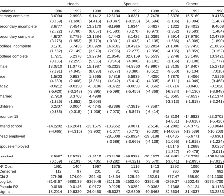
On the other hand the hours of work equation corresponds to the “Tobit type I” model in Amemiya’s classification where the variable is observed only if it is positive. In this case, the parameters of interest could be estimated using a standard censored regression Tobit model. This strategy is consistent though not fully efficient. In any case, the efficiency loss is not necessarily significant for a small sample. The results of the estimation are shown in table 2.7.
Unobservables
are rescaled by σt´/σt, where σ is the estimated standard deviation of the wage equation. This
captures the effect of differences between years in dispersion in the unobservable factor affecting wages, which include non-observables factors and their market value.15
To study employment effects the decomposition methodology requires simulating earnings for people who do not work. Since we do not observe wages we cannot apply equations (11)-(12) to estimate the unobservables. For each individual in that situation, we assign as “error term” a random draw from the bivariate normal distribution implicit in the wage-labor supply model (11)-(12), whose parameters are consistently estimated by the Heckman procedure. Residuals are sampled from the distribution of unobservables but conditional on the fact that the behavior of the individual is observed. That is, error terms are drawn from the bivariate normal distribution and a prediction (based on observable characteristics, estimated parameters and sampled errors) is computed for wages and hours worked. If the resulting prediction yields positive hours worked (so the prediction is inconsistent with observed behavior in this group), the error term is sampled again until non-positive hours of work are predicted.
Individual characteristics
For the estimation of the education effect it is necessary to simulate the educational structure of year
t´ on year t population since we do not have the same individuals in both years. Instead of following Bourguignon et al. (1999) and estimating a parametric equation that relates individual educational level to other individual characteristics (basically age and gender), we apply a rough non parametric mechanism. We divide the adult population in ten homogeneous groups by gender and age and then we replicate the educational structure of a given cell in year t’ into the corresponding cell in year t.
5. Results
This section reports the results of performing the decomposition described in section 3 using the estimation strategy outlined in section 4. The objective is to shed light over the quantitative relevance of the various phenomena discussed in section 2 on inequality changes in period 1986-1998.
Before showing the results two explanations are in order. First, the decompositions are path dependent. Hence, we report the results using alternatively t and t’ as the base year. Second, the simulations are carried out for the whole distribution. To save space we only show the results for the Gini coefficient. There are not significant variations when other indices are used.16
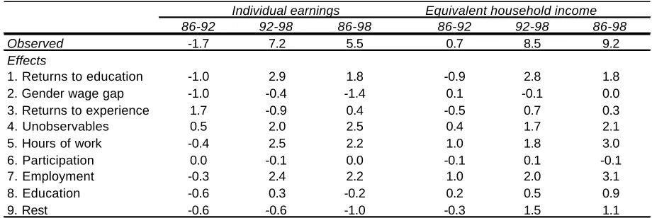
Tables 5.1 to 5.3 show the results both with t and t´ as base years. Table 5.4 reports the average of these results.17 A positive number indicates an unequalizing effect. A large number
15
It is important to remark that under bivariate normal assumption implicit in the Heckman model, once the correlation between unobservables affecting wages and hours worked is kept constant, all remaining effects on unobservables on wages come through the variance. Machado and Mata (1998) allow for hetereogeneous behavior of the error term using quantile regression methods.
16
See our companion paper.
17
compared to the other figures in the column suggests a significant effect. For instance, the returns-to-education effect on the individual earnings distribution in the 1992-1998 period is 2.9. This roughly means that the Gini would have increased 2.9 points if only the returns to education (i.e. the coefficients of the educational dummies in the wage equation) had changed between those years. The number 2.9 tells us two things: (i) since it is a positive number, it implies that the returns-to-education effect was inequality-increasing, and (ii) since it is large compared to the other numbers in the column, it indicates that the change in returns to education was a very significant factor affecting inequality.
Table 5.4
Decomposition of the change in the Gini coefficient Average results changing the base year
Individual earnings Equivalent household income
86-92 92-98 86-98 86-92 92-98 86-98
Observed -1.7 7.2 5.5 0.7 8.5 9.2
Effects
1. Returns to education -1.0 2.9 1.8 -0.9 2.8 1.8
2. Gender wage gap -1.0 -0.4 -1.4 0.1 -0.1 0.0
3. Returns to experience 1.7 -0.9 0.4 -0.5 0.7 0.3
4. Unobservables 0.5 2.0 2.5 0.4 1.7 2.1
5. Hours of work -0.4 2.5 2.2 1.0 1.8 3.0
6. Participation 0.0 -0.1 0.0 -0.1 0.1 -0.1
7. Employment -0.3 2.4 2.2 1.0 2.0 3.1
8. Education -0.6 0.3 -0.2 0.2 0.5 0.9
9. Rest -0.6 -0.6 -1.0 -0.3 1.5 1.1
Source: Author’s calculations based on the EPH, Greater Buenos Aires, September 1986, 1992, 1998.
1. Returns to education
Table 5.4 confirms the presumptions of section 2. Changes in the returns to education had an equalizing effect on the individual earnings distribution between 1986 and 1992 and a strong unequalizing effect in the next six years. The effects on the equivalent income distribution were similar. Over the whole period 1986-1998, changes in the returns to education (in terms of hourly wages) represented an important inequality-increasing factor.
2. Gender wage gap
As it was expected, changes in the gender parameter of the wage equation implied an equalizing effect on the individual earnings distribution. During the last decade the gender gap has substantially shrunk. Given that women earn less than men, that movement had an unambiguous inequality-decreasing effect on the earnings distribution.
between 1992 and 1998. The returns-to-education effect is 2.9. This is the average over two numbers: (i) the
difference between the Gini that results from applying 1998 vector βed of educational dummies to the 1992
However it is interesting to notice that the gender effect becomes negligible in the equivalent household labor income distribution.18 Two factors combine to generate that result. On the one hand
female workers are more concentrated in the upper part of the distribution than men (partly because of their own labor decisions) and hence a relative wage change implies an increase in household income inequality.19 However, on the other hand a proportional wage increase for all females is more
relevant in low-income families since women’s earnings are a more significant part of total resources in those households than in rich families. An extreme example is the disproportionate number of poor households headed by working women.
3. Returns to experience (age)
Changes in the returns to experience (age) implied a non negligible unequalizing effect on the earnings distribution during the period 1986-1992. A brief explanation is in order. Changes in the returns to experience within family categories (head, spouses and rest) did not have a clear effect on the earnings distribution of each category. For instance, the Gini coefficient for heads does not significantly change when the 1992 experience parameters of the wage equation are used to simulate earnings in 1986. The same is true for the other categories. However, recall from section 2 that changes in returns to experience between 1986 and 1992 tended to increase wages for heads and decrease them for spouses. Since heads are mostly men and spouses are nearly exclusively women, those changes implied an inequality-increasing effect. An opposite pattern shows up between 1992 and 1998, thus implying an equalizing effect.20
4. Unobservables
Changes in endowments and returns to unobservable factors have implied unequalizing changes in wages, which have translated into unequalizing changes in the individual earnings and equivalent household labor income distributions. These effects were particularly strong in the 1992-1998 period. The results of the decompositions suggest that the increase in the dispersion of unobservables was one of the main factors affecting earnings and household inequality over the period under analysis.
5. Employment
We perform three simulations to assess the relevance of employment changes on inequality. In all of them the distribution in the base year is simulated using the parameters of the Tobit employment equation of the other year. In the employment and participation effects, people with non positive simulated hours of work are assigned zero earnings. People who work in the simulation are assigned
18
It even becomes unequalizing during 1986-1992.
19
While 44% of working women are in the highest-income quintile of the equivalent household labor income distribution, only 25% of men are in that quintile. On the other extreme 6% of working women are in the lowest-income quintile while 9% of men are there.
20
the actual base year wage and the simulated worked hours in the employment effect and the actual worked hours in the participation effect.21 The third simulation is intended to single out the impact of
changes in hours worked. We ignore people who change labor status (i.e. we keep their actual earnings) and change hours of work to individuals who work both in the base year and in the simulation.
Most of the action takes place between 1992 and 1998. A strong unequalizing employment effect shows up in the individual earnings distribution. Notice that since we exclude those individuals with zero earnings from that distribution, the employment effect is basically the result of relative changes in the number of hours of work. The figures for the hours-of-work and participation effects confirm this assertion. As it was discussed in section 2 the nineties witnessed a substantial fall in hours of work by low-income workers and an increase for the rest. It seems that this fact has had a very significant impact on the earnings distribution.
Unemployment rate skyrocketed in mid-nineties and has remained very high since then. It is a widespread belief that changes in labor market participation are the main cause of the strong increase in household inequality. Results in the second panel of table 5.4 suggest to scale down those conclusions. The participation effect is positive but negligible. In contrast, changes in hours of work seem to have had a very significant unequalizing effect on the household income distribution.
A couple of reasons contribute to reduce the effect of the great increase in unemployment on household inequality. The first one was mentioned in section 2. During 1992-1998 the unemployment rate jumped but the employment rate did not change very much, implying a minor change in the number of individuals without earnings. As it was stressed before, this is the relevant number for household inequality, not the number of unemployed people. The second point is that the new unemployed (those who did not work in 1998 but that would have worked with the 1992 parameters) had extremely low individual incomes in 1992 (just 10% of the rest), but equivalent household incomes not so far from the median (75% of the median). This implies that in the simulation using the 1992 parameters the change in labor status (from unemployed to employed) of some individuals would not have a very strong effect on household inequality since (i) anyway those individuals had very low incomes, and (ii) they were not very concentrated in the lower tail of the household income distribution.
Naturally, the role of unemployment as the main source of the increase in inequality can be stressed again if it is argued that the fall in the relative wages of the poorest workers was generated by a relative increase in the unemployment rate in that group. However, the evidence on this point is far from being conclusive (see table 2.9).22
6. Education
21
Some people do not work in the base year but do work in the simulation. For those individuals we simulate the base year worked hours and wages using the base year parameters of equations (11) and (12) and adding error terms obtained by following the procedure described in section 4.
22
Argentina has witnessed a dramatic change in the educational composition of its population in the last two decades. However, according to the results shown in table 5.4 that change did not have a substantial effect on earnings inequality. This is not a surprising result according to our discussion in section 2. The education effect is slightly more unequalizing on the household labor income distribution, probably as a result of the positive correlation of educational levels within the household. However the effect is not very significant either.
7. Other factors and residuals
The last row in table 5.4 is calculated as a residual. It encompasses the effects of interactions terms and of many factors not considered in the analysis. According to table 5.4 in general this term is lower than most of the other terms in the decomposition, implying either that the factors not considered in the analysis are not extremely important or that they tend to compensate each other.
6. Concluding remarks
This papers contributes to a highly discussed topic in Argentina -the increase in income inequality- by using a microeconometric decompositions methodology. This technique allows us to assess the relevance of various factors that affected inequality in the last 12 years.
The results of the paper suggest that the small change in inequality between 1986 and 1992 is the result of mild forces that tend to compensate each other. In contrast, between 1992 and 1998 nearly all effects played in the same direction. Changes in the returns to education and experience, changes in the endowments of unobservable factors and their remunerations, changes in labor supply, and the transformation of the educational structure of the population have all had some role in increasing inequality in Argentina to unprecedented levels. Even the decrease in the wage gap between genders, which is a potential force for reducing inequality, has not induced a significant decrease in household income inequality.
References
Altimir, O., Beccaria, L. and González Rozada, M. (2000). La evolución de la distribución del ingreso familiar en la Argentina. Documento de trabajo de la Maestría en Finanzas Públicas Provinciales y Municipales, UNLP.
Amemiya, T. (1985). Advanced Econometrics, Harvard University Press.
Bouillon, C., Legovini, A. and Lustig, N. (1998). Rising inequality in Mexico: returns to household characteristics and the "Chiapas effect". Mimeo.
Bourguignon, F., Ferreira, F. and Lustig, N. (1998). The microeconomics of income
distribution dynamics in East Asia and Latin America. IDB-World Bank Research Proposal.
Bourguignon, F., Fournier, M., and Gurgand, M. (1999). Fast development with an stable income distribution: Taiwan, 1979-1994. Mimeo.
Buhmann, B., Rainwater, G. Schmaus, G. y Smeeding, T. (1988). Equivalence scales, well
being, inequality and poverty: sensitivity estimates across ten countries using the Luxembourg Income Study database. Review of Income and Wealth 34, 115-142.
Ferreira, Francisco y Paes de Barros, Ricardo (1999). Climbing a moving mountain: explaining the decline in income inequality in Brazil from 1976 to 1996. Mimeo.
Gasparini, L. (1999). Desigualdad en la distribución del ingreso y bienestar. Estimaciones para la Argentina. En La distribución del ingreso en la Argentina, FIEL, Buenos Aires, 35-83.
Gasparini, L. y Sosa Escudero, W. (1999). Assessing aggregate welfare: growth and inequality in Argentina. Documento de trabajo, Universidad Nacional de La Plata.
Gasparini, L., Marchionni, M. y Sosa Escudero, W. (1999). La distribución del ingreso en la
Argentina. Un análisis en base a descomposiciones microeconométricas. Convenio Ministerio de Economía de la Provincia de Buenos Aires-Facultad de Ciencias Económicas, Universidad Nacional de La Plata.
Heckman, J. (1974). Shadow Prices, Market Wages, and Labor Supply. Econometrica. 42, 4.
Juhn, C, Murphy, K. y Pierce, B. (1993). Wage inequality and the rise in returns to skill.
Journal of Political Economy 101 (3), 410-442.
Kuznets, S. (1955). Economic growth and income inequality. American Economic Review, 45, 1-28.
Lee, H. (1999). Article on income distribution in Argentina in the Argentina Poverty Assessment. The World Bank.
Llach, J. y Montoya, S. (1999). En pos de la equidad. Pobreza y distribución del ingreso en la Argentina.
Machado, J. y Mata, J. (1998). Sources of increased inequality. Mimeo. Universidade Nova de Lisboa.
Table 2.1 Gini coefficient
Individual labor income and equivalent household labor income Greater Buenos Aires, September 1986, 1992 and 1998
1986 1992 1998
Individual labor income 39.4 37.7 44.9 Equivalent household labor income 40.3 41.0 49.5
Source: Author’s calculations based on the EPH.
Table 2.2
Hourly earnings by educational levels
Greater Buenos Aires, September, 1986, 1992, 1998.
Means ($ 1998) Change (%)
1986 1992 1998 92-86 98-92 98-86
Primary incomplete 6.6 5.7 5.3 -13.6 -6.8 -19.5
Primary complete 7.7 6.3 5.9 -18.1 -6.0 -23.0
Secondary incomplete 9.2 6.8 6.6 -26.1 -2.8 -28.1
Secondary complete 11.6 9.1 9.1 -21.2 -0.4 -21.5
College incomplete 14.5 11.9 10.6 -17.5 -11.1 -26.7
College complete 24.1 16.3 19.4 -32.3 19.1 -19.4
Total 10.4 8.4 9.2 -19.0 9.3 -11.4
[image:21.612.109.519.346.464.2]Table 2.3
Log hourly earnings equation
Variables Heads Spouses Others
Earnings Eq. 1986 1992 1998 1986 1992 1998 1986 1992 1998 primary complete 0.2150 0.2162 0.1828 0.0393 -0.1731 0.0575 0.0407 0.3349 0.0417 (5.496) (4.011) (2.978) (0.496) (-1.695) (0.462) (0.441) (2.884) (0.287) secondary incomplete 0.3994 0.3367 0.3630 0.2241 -0.0243 0.2306 0.2278 0.4361 0.1366 (9.206) (5.661) (5.620) (2.342) (-0.211) (1.848) (2.400) (3.795) (0.953) secondary complete 0.6219 0.6229 0.6534 0.5595 0.2652 0.4841 0.4053 0.5726 0.3646 (12.649) (10.185) (9.664) (6.720) (2.445) (3.861) (3.927) (4.546) (2.447) college incomplete 0.9121 0.9516 0.9382 0.6446 0.5173 0.6579 0.5646 0.7100 0.6699 (15.469) (12.713) (12.714) (5.210) (3.666) (4.347) (5.289) (5.919) (4.592) college complete 1.3079 1.2607 1.4634 0.8607 0.5764 0.9607 0.7439 0.8109 0.9456 (22.778) (18.242) (20.282) (7.824) (4.183) (5.600) (5.577) (5.432) (5.830) male 0.2915 0.1834 0.1675 -0.1865 0.2626 0.2859 0.0454 0.0701 0.1678 (5.106) (3.707) (3.474) (-0.774) (1.280) (1.706) (0.827) (1.405) (3.250) age 0.0401 0.0546 0.0452 0.0413 0.0343 0.0454 0.0766 0.0797 0.0846 (3.969) (4.882) (3.951) (2.120) (1.533) (2.028) (4.351) (4.267) (4.138) age2 -0.0004 -0.0006 -0.0004 -0.0005 -0.0004 -0.0005 -0.0009 -0.0009 -0.0011 (-3.295) (-4.661) (-3.155) (-2.057) (-1.393) (-1.813) (-3.646) (-3.545) (-3.735)
younger 18 -0.0218 -0.0338 -0.3601
(-0.250) (-0.406) (-2.811) constant 0.5599 0.1959 0.2051 1.0778 1.1095 0.6169 0.1849 -0.2793 -0.3190 (2.400) (0.806) (0.792) (2.554) (2.283) (1.178) (0.577) (-0.749) (-0.799) Selection Equation (dep. var.=1 if hourly earnings>0)
primary complete 0.2931 0.2212 0.3955 -0.3295 -0.0513 -0.1975 0.2137 0.5917 0.2573 (2.240) (1.429) (3.052) (-3.289) (-0.381) (-1.346) (1.203) (2.874) (1.126) secondary incomplete 0.3494 0.5737 0.4556 -0.1980 0.0129 0.0398 0.2258 0.8538 0.2308 (2.238) (2.987) (3.234) (-1.612) (0.083) (0.258) (1.215) (4.015) (1.021) secondary complete 0.4875 0.5575 0.5866 -0.0736 0.1556 0.2299 0.4315 0.7899 0.4376 (2.580) (2.827) (3.736) (-0.639) (1.066) (1.489) (1.901) (3.296) (1.829) college incomplete 0.4760 1.0563 0.4125 0.4776 0.5239 0.4153 0.8123 1.5396 0.5657 (1.827) (3.318) (2.177) (2.355) (2.433) (2.102) (3.441) (5.794) (2.284) college complete 1.2176 1.0181 0.8111 0.7033 1.0577 1.3115 0.8274 1.3888 0.8389 (3.085) (3.750) (4.537) (4.467) (5.620) (7.588) (2.101) (3.766) (2.752) male 0.8594 0.7840 0.6528 1.2982 1.7185 1.3967 0.8164 0.4630 0.5007 (5.175) (4.001) (5.263) (2.235) (2.970) (5.353) (8.451) (4.703) (6.182) age 0.1099 0.1141 0.1045 0.1288 0.1757 0.1203 0.1960 0.1686 0.2719 (3.160) (3.012) (3.748) (4.907) (5.577) (4.279) (5.682) (4.836) (9.111) age2 -0.0014 -0.0016 -0.0014 -0.0017 -0.0023 -0.0015 -0.0029 -0.0022 -0.0036 (-3.541) (-3.589) (-4.269) (-5.117) (-5.668) (-4.353) (-6.385) (-4.832) (-8.656) married 0.1986 0.1559 0.0588 -0.7813 -0.4060 -0.4761 (1.204) (0.841) (0.477) (-4.386) (-2.373) (-3.360) children -0.0087 -0.0178 -0.0464 -0.1929 -0.1797 -0.1768
(-0.202) (-0.442) (-1.387) (-6.496) (-5.460) (-5.477)
younger 18 -0.5983 -0.3063 -0.5995
(-3.823) (-1.925) (-4.087) attend school -0.8669 -1.0407 -0.5569 -0.3036 0.3501 0.2020 -1.6477 -1.7389 -0.9050 (-2.850) (-3.280) (-2.509) (-0.963) (1.040) (0.900) (-11.458) (-11.237) (-7.556) head employed -0.7922 -0.6382 -0.6148 -0.0351 -0.1624 -0.2210 (-3.982) (-3.314) (-4.386) (-0.212) (-1.112) (-1.951)
spouse employed -0.0763 -0.0005 0.0488
(-0.706) (-0.005) (0.547) constant -1.3555 -1.3567 -1.3239 -1.5356 -2.7184 -1.8346 -2.6080 -2.6912 -4.0987 (-1.892) (-1.682) (-2.296) (-3.015) (-4.571) (-3.390) (-4.233) (-4.358) (-8.127) Nº Obs. 1961 1404 1967 1575 1116 1413 1292 1090 1631 Chi 2 153.77 124.61 148.96 164.62 154.13 303.14 767.13 590.80 861.41 Log Lik. -1888.35 -1368.31 -2281.71 -1311.55 998.04 -1354.19 -841.52 -769.56 -1191.27 Rho 0.2179 0.6786 0.1247 -0.1691 0.0379 -0.1035 0.1705 0.3726 0.3600 Sigma 0.5562 0.5747 0.6361 0.5603 0.5492 0.6434 0.4848 0.4770 0.5569 Lambda 0.1212 0.3900 0.0793 -0.0948 0.0208 -0.0666 0.0827 0.1777 0.2005
Table 2.4
Hourly earnings by gender
Greater Buenos Aires, September, 1986, 1992, 1998.
Means ($ 1998) Change (%)
1986 1992 1998 92-86 98-92 98-86
Female 9.3 8.1 9.0 -12.6 10.2 -3.7
Male 10.8 8.5 9.3 -21.2 9.0 -14.1
Total 10.4 8.4 9.2 -18.9 9.3 -11.4
[image:24.612.132.494.325.444.2]Source: Author’s calculations based on the EPH.
Table 2.5
Hourly earnings by age groups
Greater Buenos Aires, September, 1986, 1992, 1998.
Means ($ 1998) Change (%)
1986 1992 1998 92-86 98-92 98-86
14-19 5.0 4.7 4.3 -6.7 -7.9 -14.1
20-29 9.0 7.4 6.9 -17.4 -7.5 -23.6
30-39 11.2 9.5 9.5 -14.9 0.4 -14.5
40-49 11.9 9.4 10.8 -21.2 14.8 -9.6
50-59 9.9 8.1 11.2 -18.0 38.1 13.3
60-65 12.9 8.5 9.0 -34.1 6.7 -29.7
Total 10.4 8.4 9.2 -19.0 9.4 -11.4
Source: Author’s calculations based on the EPH.
Table 2.6
Weekly hours of work by educational levels Greater Buenos Aires, September, 1986, 1992, 1998.
Means Change (%)
1986 1992 1998 92-86 98-92 98-86
Primary incomplete 45.7 45.6 40.2 -0.3 -11.7 -12.0
Primary complete 48.5 46.8 46.5 -3.3 -0.8 -4.1
Secondary incomplete 47.0 47.0 47.5 0.1 1.0 1.1
Secondary complete 46.9 45.1 46.7 -3.9 3.5 -0.5
College incomplete 42.7 41.9 41.8 -1.9 -0.1 -2.0
College complete 42.6 42.3 42.8 -0.5 1.1 0.5
Total 46.5 45.5 45.2 -2.1 -0.8 -2.9
[image:24.612.110.519.528.646.2]Table 2.7
Hours of work equation
Heads Spouses Others
Variables 1986 1992 1998 1986 1992 1998 1986 1992 1998 primary complete 3.6994 2.9998 9.1412 -12.8134 -0.8331 -3.7478 9.5376 16.5169 9.4156 (3.059) (1.690) (4.416) (-3.047) (-0.158) (-0.694) (2.186) (3.094) (1.467) secondary incomplete 3.6777 7.4547 13.2170 -8.1969 1.6344 5.4827 6.1322 19.4012 9.4008 (2.722) (3.780) (6.057) (-1.583) (0.270) (0.973) (1.352) (3.583) (1.484) secondary complete 4.6707 3.7789 13.1584 -1.4443 8.1426 12.0399 8.5914 17.9790 12.4789 (3.075) (1.853) (5.770) (-0.301) (1.432) (2.135) (1.686) (3.009) (1.890) college incomplete 3.1701 5.7436 10.8928 16.6182 18.4916 20.2824 24.1386 39.7456 21.8096 (1.552) (2.149) (3.979) (2.095) (2.277) (2.858) (4.185) (5.859) (3.152) college complete 1.7271 5.2378 13.2734 21.8548 32.6159 36.5539 8.2748 23.1498 13.3421 (0.985) (2.255) (5.535) (3.546) (4.806) (6.181) (1.156) (3.108) (1.777) male 13.0310 11.0772 15.1987 45.2329 44.9860 43.9907 21.8135 14.8407 15.2718 (7.291) (4.845) (8.093) (2.677) (3.380) (6.512) (9.650) (6.134) (7.018) age 1.5803 0.9534 1.3565 5.4816 6.5939 4.4250 4.7870 3.4066 7.5266 (4.980) (2.468) (3.351) (4.942) (5.414) (4.335) (6.111) (4.049) (9.468) age2 -0.0212 -0.0150 -0.0186 -0.0722 -0.0850 -0.0562 -0.0714 -0.0468 -0.1020 (-5.620) (-3.248) (-3.895) (-5.098) (-5.455) (-4.368) (-6.934) (-4.130) (-8.948) married 2.7919 3.3768 4.4988 -15.8565 -7.6537 -12.1374 (1.826) (1.652) (2.608) (-3.813) (-1.818) (-3.241) children 0.2807 0.0064 -0.4745 -8.7386 -7.3819 -7.3587
(0.835) (0.015) (-1.036) (-7.070) (-5.847) (-6.414)
younger 18 -18.8104 -14.6823 -23.3702
(-4.861) (-3.618) (-5.426) attend school -14.2282 -16.2041 -13.1575 -13.9652 9.0871 2.5146 -51.2882 -54.3772 -33.9044 (-4.665) (-4.315) (-3.902) (-1.077) (0.772) (0.330) (-14.003) (-13.539) (-10.203) head employed -28.5008 -25.8924 -19.6188 -4.0485 -5.6771 -3.6361 (-3.686) (-3.669) (-4.138) (-1.095) (-1.619) (-1.224)
spouse employed -3.5146 1.2688 0.0257
(-1.327) (0.478) (0.011) constant 3.5987 17.5783 -3.6110 -70.2406 -99.8388 -70.4622 -51.8461 -43.2795 -108.5699 (0.559) (2.193) (-0.435) (-3.282) (-4.321) (-3.570) (-3.641) (-2.895) (-7.913) Nº Obs. 1961 1404 1967 1575 1116 1413 1292 1090 1631
Censored 112 97 201 81 705 848 780 609 982
Chi 2 279.96 174.00 292.40 143.34 129.49 252.91 877.47 658.90 941.1300 Log Lik -8148.67 -5880.39 -8369.46 -3111.35 -2502.00 -3352.46 -2769.37 -2602.48 -3576.4700 Pseudo R2 0.0169 0.0146 0.0172 0.0225 0.0252 0.0363 0.1368 0.1124 0.1163 sigma 18.2014 19.6320 24.0450 45.6327 42.6309 40.6468 30.5604 31.4037 33.2833
Table 2.8
Labor status by role in the household
Greater Buenos Aires, September, 1986, 1992, 1998.
Proportions by group (%)
1986 1992 1998
Heads
Employed 94.6 93.1 89.8
Unemployed 2.0 3.1 5.2
Inactive 3.4 3.8 5.0
Spouses
Employed 31.7 36.8 40.1
Unemployed 1.4 1.7 5.6
Inactive 66.9 61.5 54.3
Other
Employed 39.6 44.1 39.8
Unemployed 4.0 5.9 8.8
Inactive 56.3 50.0 51.4
All
Employed 59.4 60.9 59.5
Unemployed 2.3 3.5 6.5
Inactive 38.3 35.6 34.0
Source: Author’s calculations based on the EPH.
Table 2.9
Labor status by education
Proportions by group (%)
1986 1992 1998
Primary incomplete
Employed 60.6 53.3 55.3
Unemployed 3.1 4.6 8.5
Inactive 36.3 42.2 36.2
Primary complete
Employed 60.1 63.7 61.5
Unemployed 2.6 3.8 7.7
Inactive 37.4 32.5 30.8
Secondary incomplete
Employed 46.1 47.3 42.9
Unemployed 2.2 2.6 5.6
Inactive 51.7 50.1 51.5
Secondary complete
Employed 66.3 68.6 71.5
Unemployed 1.5 3.9 6.3
Inactive 32.2 27.5 22.2
College incomplete
Employed 65.9 66.0 60.7
Unemployed 2.6 4.5 6.8
Inactive 31.5 29.6 32.5
College complete
Employed 86.4 88.3 88.8
Unemployed 1.4 1.9 4.8
Inactive 12.2 9.9 6.4
All
Employed 59.4 60.9 59.5
Unemployed 2.3 3.5 6.5
Inactive 38.3 35.6 34.0
Table 2.10
Sample composition by educational level
(proportions in the sample)
Greater Buenos Aires, September, 1986, 1992, 1998.
1986 1992 1998
Primary incomplete 15.4 11.0 7.3
Primary complete 32.0 31.1 25.2
Secondary incomplete 26.0 26.8 30.6
Secondary complete 13.5 15.8 15.2
College incomplete 7.1 8.1 11.7
College complete 6.0 7.3 10.0
Table 5.1
Decompositions of the change in the Gini coefficient Individual earnings and equivalent household income
Greater Buenos Aires, 1986-1992
Using 1992 coefficients
Individual earnings Equivalent income
Level Change Level Change
1986 observed 39.4 40.3
1992 observed 37.7 -1.7 41.0 0.7
Effects
1. Returns to education 38.9 -0.5 39.7 -0.6
2. Gender wage gap 38.4 -1.0 40.4 0.1
3. Returns to experience 41.5 2.1 40.0 -0.3
4. Unobservables 39.9 0.5 40.7 0.4
5. Hours of work 39.8 0.4 41.7 1.4
6. Participation 39.4 0.0 40.1 -0.3
7. Employment 39.8 0.4 41.6 1.3
8. Education 39.2 -0.2 40.5 0.1
9. Rest -1.8 -0.5
Using 1986 coefficients
Individual earnings Equivalent income
Level Change Level Change
1986 observed 39.4 -1.7 40.3 0.7
1992 observed 37.7 41.0
Effects
1. Returns to education 39.2 -1.5 42.2 -1.2
2. Gender wage gap 38.8 -1.1 40.9 0.1
3. Returns to experience 36.4 1.3 41.7 -0.7
4. Unobservables 37.2 0.5 40.7 0.3
5. Hours of work 38.8 -1.2 40.4 0.6
6. Participation 37.6 0.1 41.0 0.0
7. Employment 38.7 -1.1 40.3 0.7
8. Education 38.6 -1.0 40.8 0.2
9. Rest 0.7 -0.1
Average changes
Individual Equivalent earnings income
Observed 86-92 -1.7 0.7
Effects
1. Returns to education -1.0 -0.9 2. Gender wage gap -1.0 0.1 3. Returns to experience 1.7 -0.5 4. Unobservables 0.5 0.4 5. Hours of work -0.4 1.0 6. Participation 0.0 -0.1
7. Employment -0.3 1.0
8. Education -0.6 0.2
Table 5.2
Decompositions of the change in the Gini coefficient Individual earnings and equivalent household income
Greater Buenos Aires, 1992-1998
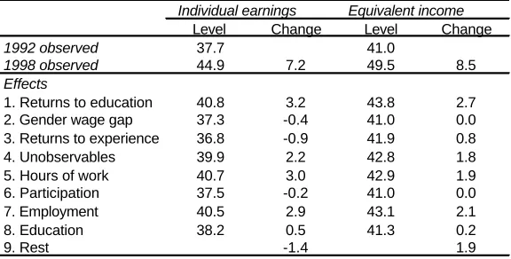
Using 1998 coefficients
Individual earnings Equivalent income
Level Change Level Change
1992 observed 37.7 41.0
1998 observed 44.9 7.2 49.5 8.5
Effects
1. Returns to education 40.8 3.2 43.8 2.7
2. Gender wage gap 37.3 -0.4 41.0 0.0
3. Returns to experience 36.8 -0.9 41.9 0.8
4. Unobservables 39.9 2.2 42.8 1.8
5. Hours of work 40.7 3.0 42.9 1.9
6. Participation 37.5 -0.2 41.0 0.0
7. Employment 40.5 2.9 43.1 2.1
8. Education 38.2 0.5 41.3 0.2
9. Rest -1.4 1.9
Using 1992 coefficients
Individual earnings Equivalent income
Level Change Level Change
1992 observed 37.7 7.2 41.0 8.5
1998 observed 44.9 49.5
Effects
1. Returns to education 42.2 2.7 46.5 3.0 2. Gender wage gap 45.3 -0.4 49.6 -0.1 3. Returns to experience 45.9 -1.0 48.8 0.7
4. Unobservables 43.1 1.8 48.0 1.5
5. Hours of work 43.0 1.9 47.8 1.7
6. Participation 44.8 0.1 49.2 0.3
7. Employment 42.9 2.0 47.5 2.0
8. Education 44.8 0.1 48.7 0.8
9. Rest 0.2 1.1
Average changes
Individual Equivalent earnings income
Observed 92-98 7.2 8.5
Effects
1. Returns to education 2.9 2.8 2. Gender wage gap -0.4 -0.1 3. Returns to experience -0.9 0.7 4. Unobservables 2.0 1.7 5. Hours of work 2.5 1.8 6. Participation -0.1 0.1
7. Employment 2.4 2.0
8. Education 0.3 0.5
Table 5.3
Decompositions of the change in the Gini coefficient Individual earnings and equivalent household income
Greater Buenos Aires, 1986-1998
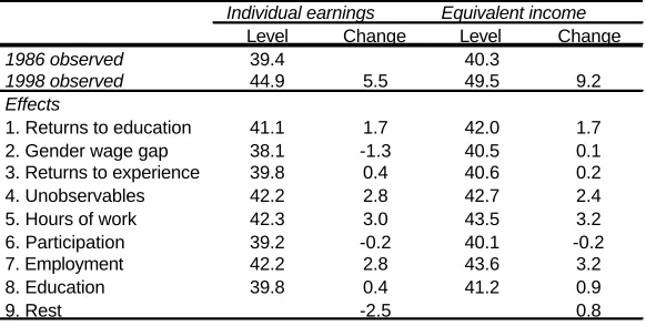
Using 1998 coefficients
Individual earnings Equivalent income
Level Change Level Change
1986 observed 39.4 40.3
1998 observed 44.9 5.5 49.5 9.2
Effects
1. Returns to education 41.1 1.7 42.0 1.7
2. Gender wage gap 38.1 -1.3 40.5 0.1
3. Returns to experience 39.8 0.4 40.6 0.2
4. Unobservables 42.2 2.8 42.7 2.4
5. Hours of work 42.3 3.0 43.5 3.2
6. Participation 39.2 -0.2 40.1 -0.2
7. Employment 42.2 2.8 43.6 3.2
8. Education 39.8 0.4 41.2 0.9
9. Rest -2.5 0.8
3. Employment Using 1986 coefficients
Individual earnings Equivalent income
Level Change Level Change
1986 observed 39.4 5.5 40.3 9.2
1998 observed 44.9 49.5
Effects
1. Returns to education 43.0 1.9 47.6 1.9 2. Gender wage gap 46.4 -1.5 49.7 -0.2 3. Returns to experience 44.5 0.4 49.2 0.3
4. Unobservables 42.7 2.2 47.7 1.8
5. Hours of work 43.5 1.4 46.7 2.8
6. Participation 44.7 0.2 49.4 0.1
7. Employment 43.3 1.6 46.5 3.0
8. Education 45.7 -0.8 48.5 1.0
9. Rest 0.4 1.3
Average changes
Individual Equivalent earnings income
Observed 86-98 5.5 9.2
Effects
1. Returns to education 1.8 1.8 2. Gender wage gap -1.4 0.0 3. Returns to experience 0.4 0.3
4. Unobservables 2.5 2.1
5. Hours of work 2.2 3.0
6. Participation 0.0 -0.1
7. Employment 2.2 3.1
8. Education -0.2 0.9
Figure 2.1
Gini coefficient of equivalent household income Greater Buenos Aires, September 1985-1998
38 39 40 41 42 43 44 45 46 47 48
1985 1986 1987 1988 1989 1990 1991 1992 1993 1994 1995 1996 1997 1998
Gini
Figure 2.2
Hourly earnings-education profiles Men 40 years old
Household heads
0 5 10 15 20 25
prii pric seci secc coli colc
education
hourly earnings
Other members
0 2 4 6 8 10 12 14
prii pric seci secc coli colc
education
hourly earnings
____
1986__ __
1992_ _ _
1998Note: prii=primary incomplete, pric=primary complete, seci=secondary incomplete
Figure 2.3
Hourly earnings-education profiles Women 40 years old
Spouses
0 2 4 6 8 10 12 14 16 18
prii pric seci secc coli colc
education
hourly earnings
Other members
0 2 4 6 8 10 12 14
prii pric seci secc coli colc
education
hourly earnings
____
1986__ __
1992_ _ _
1998Note: prii=primary incomplete, pric=primary complete, seci=secondary incomplete
Figure 2.4
Weekly hours of work by educational level
Male heads 40 years old
20 25 30 35 40 45 50 55
prii pric seci secc coli colc
education
weekly hours of work
Female spouses 40 years old
0 5 10 15 20 25 30 35 40 45 50
prii pric seci secc coli colc
education
weekly hours of work
____
1986__ __
1992_ _ _
1998Note: prii=primary incomplete, pric=primary complete, seci=secondary incomplete