GENDER GAPS IN UNEMPLOYMENT RATES IN ARGENTINA
ANA CAROLINA ORTEGA MASAGUÉ
RESUMEN
Clasificación JEL: J16, J64
Utilizando datos de la Encuesta de Hogares para el periodo 1995-2001, se estudian los factores que explican el diferencial entre las tasas de desempleo de hombres y mujeres en Argentina. Se encuentra que este diferencial viene explicado no por diferencias en las características de ambos grupos, sino por diferencias en los rendimientos de mercado de sus características, en especial, aquellos asociados al estado civil. Por tanto, las diferencias en el comportamiento de hombres y mujeres, así como las prácticas de los empresarios en relación al género de los trabajadores se encuentran detrás de este diferencial. Sin embargo, la importancia relativa de estos dos factores en la explicación de dicho diferencial no está clara.
Palabras clave: brecha de género, tasas de desempleo.
ABSTRACT
JEL Classification: J16, J64
Using data from the Argentinean Household Survey for the period 1995-2001, I study the factors that explain the gender gap in unemployment rates. Using a microeconometric decomposition technique, I find that the gender gap in unemployment rates is explained not by differences in the characteristics of men and women but by differences in the labor market returns to their characteristics, especially those associated to the marital status. Hence, differences in men’s and women’s behaviour and the practices of employers towards gender are behind the gender gap. However, the relative importance of these two factors in explaining the gap is not totally clear.
GENDER GAPS IN UNEMPLOYMENT RATES IN ARGENTINA1
ANA CAROLINA ORTEGA MASAGUÉ2
I. Introduction
The literature that studies gender gaps in labor force participation rates and wages, as well as the one that analyzes occupational segregation by gender are by now very large, covering different countries and time periods.3 In contrast,
the studies that examine gender gaps in unemployment rates are much scarcer. Moreover, the empirical evidence on this matter is not totally conclusive, and to a large extent refers to developed countries where the characteristics of the labor market institutions and participants are different from those in less developed countries.
During the last years, the evolution of the unemployment rate in Argentina showed some peculiarities that make the Argentinean labor market an interesting case of study. The 1990s was a decade of important changes for the Argentinean economy. Structural reforms based on the Convertibility Law, a widespread privatization and deregulation process, and a significant trade and financial liberalization affected all aspects of the economy. Following the reforms of the early 1990s, most of the macro variables showed positive changes, such as higher growth and much lower inflation. However, unemployment grew during the early part of the decade and has remained high
1 I am grateful to Juan Francisco Jimeno, Daniel Kotzer, Raquel Carrasco, José María Labeaga, Cristina Fernández, Juan Ramón García and two anonymous referrers for their helpful comments and suggestions. All remaining errors are my own. Contact the author at [email protected].
2 Universidad de Alcalá de Henares
3 For a survey of these topics see Altonji and Blank (1999). Some of the most recent articles that study gender wage gaps are Blau and Kahn (2004) for the United States (US), Beblo et al.
ever since. 4 Moreover, the steep increase in the level of unemployment was
accompanied by a notable increase in the gender gap in unemployment rates, which reached more than 5 percentage points in 1996 (see Figure B1).This strong rise has spurred some concerns about the underlying causes of the gender gap in unemployment rates.
In response to this concern, the aim of this paper is to investigate the factors that explain the gender gaps in unemployment rates in Argentina during the period 1995-2001. In other words, I am interested in studying the reasons why women, once they have decided they want a job, have lower probabilities of being employed than men.
The economic theory suggests that there are many possible explanations for the gender gap in unemployment rates. On the demand side, discrimination has been pointed out as one of the factors that would explain the higher female unemployment rate. The economic models distinguish two main sources of discrimination. The first one, formulated by Becker, refers to the prejudices that, at least, part of the employers might have against women. The second one refers to the so called statistical discrimination. It arises as a consequence that employers, in the presence of imperfect information, assume that women, on average, have a lower level of labour market attachment and are less qualified than men. On the supply side, the lower labor market attachment of women, reflected in a lower job search intensity and human capital accumulation and in higher movements into and out of the labor force, a higher reservation wage for women, as well as their different characteristics have been some of the factors mentioned as plausible causes of the gender gap in unemployment rates.
Political measures intended for eliminating women’s inferiority in the labor market will depend on the causes of the gender gap in unemployment rates. These measures will not only improve women’s relative position in the labor market, but they will also contribute to mitigate the serious problem of unemployment, increasing the employment opportunities of an important part of the labor force. Thus, understanding this phenomenon becomes a very important question.
The rest of the paper is structured as follows. In the next section I review the existing literature on gender gaps in unemployment rates. In order to analyze the factors that explain the gender gap in unemployment rates I use both a static and a dynamic approach, which are discussed in Section III. Firstly, I estimate a random effects probit model for the probability of being unemployed. Secondly, I analyze the flows between labor market states. Given the importance of the flows from unemployment to employment in explaining gender gaps in unemployment rates, I estimate a duration model for the probability of leaving unemployment. Finally, in each case I carry out a decomposition analysis based on the Oaxaca-Blinder technique. For doing this analysis, I rely on data from the Argentinean Household Survey for the period 1995-2001. These data are described in Section IV. Section V presents the results of the empirical analysis. Overall, I find that the gender gap in unemployment rates is explained not by differences in the observed and unobserved characteristics of men and women but by differences in the labor market returns to their characteristics. Hence, differences in men’s and women’s behaviour and the practices of employers towards gender are behind the gender gap in unemployment rates in Argentina. However, the relative importance of these two factors in explaining the gender gap in unemployment rates is not totally clear. Finally, section VI concludes.
II. Literature Review
The economic literature has devoted relatively little efforts to the study of gender gaps in unemployment rates. To keep this section at a manageable size I focus on the studies that specifically refer to gender gaps in unemployment rates.
concludes that an important part of the observed differential could be attributed to the definition and methodology used to calculate unemployment rates rather than to discrimination of employers against women.
However, in the 1980s the difference between male and female unemployment rates in the United States virtually disappeared. Then, the economic literature focuses on analyzing the possible causes of the equality of both rates. DeBoer and Seeborg (1989) study the changes in the probabilities of transition between different labor market states. Using data from the Bureau of Labor Statistics (BLS), the authors find that about half of the narrowing of the unemployment rates differential during the period 1968-1985 was due to the increasing labor force attachment of women and the decreasing attachment of men. The other half reflects changes in men’s and women’s tendencies to move between employment and unemployment, attributed primarily to the decline of male-dominated industries. Using data from the CPS, Mohanty (1998) obtains that the disappearance of the gap between male and female unemployment probabilities results partly from a considerable decline in hiring discrimination against females during the last two decades. This study also finds that the growth of employment in government and in the service sector, and migration of workers from the South to other regions have contributed significantly to the convergence of male and female unemployment rates. More recently, using the same database, Mohanty (2003) establishes that the ability of employers to pay lower wages to women raises average female employment probabilities which, in turn, yield lower female unemployment rates. Then, wage discrimination, among other factors, would be explaining the equality between male and female unemployment rates. Therefore, the equality of male and female unemployment rates should not be confused with absence of discrimination against women.
In a European framework, using data from the European Community Household Panel (ECHP), Azmat et al. (2006) show that in countries where there is a large gender gap in unemployment rates, particularly the Mediterranean countries, there is a gender gap in both flows from employment to unemployment and from unemployment to employment. They investigate different hypotheses about the sources of these gaps, concluding that differences in human capital accumulation between men and women interacted with labor market institutions are an important part of the explanation of the gender gap in unemployment rates in the Mediterranean countries.
Also using data from the ECHP for the period 1994-1998, Eusamio (2004) studies the causes of the large differential that exists between male and female unemployment rates in Spain, extending the analysis to the Portuguese case. When studying the empirical determinants of the hazard rates from employment and unemployment of men and women, she finds that women have more difficulties to leave unemployment and a higher probability of leaving employment, at least during the first year in each state. In addition, using a non-linear Oaxaca decomposition, she obtains evidence that men and women have similar characteristics that, nonetheless, are rewarded differently.
Concerning transition countries, Ham et al. (1999) investigate the reasons why women’s unemployment rate is above men’s in the Czech and Slovak Republics. They find that the differences between men’s and women’s probabilities of leaving unemployment are explained more by differences in returns to characteristics than by differences in observed characteristics. Therefore, they conclude that differences in men’s and women’s behaviour and the practices of employers and institutions towards gender are dominating the differences between men’s and women’s exit rates from unemployment in both countries. Finally, Lauerová and Terrell (2002) analyze the determinants of the gender differences in unemployment rates in post-communist economies, specially the Czech Republic. When analysing the flows between labor market states, they find that an important part of the gender gap in unemployment rates results from married women’s lower probability of moving from unemployment to employment and from single women’s lower probability of moving from inactivity to employment.
III. Empirical Approach
In order to study the gender gap in unemployment rates, I follow both a static approach and a dynamic approach. In the first case, I estimate a random effects probit model for the probability of being unemployed (conditional on being in the labor force since I am looking at unemployment rates). In the second case, I analyze the flows between labor market states. I focus on the flows from unemployment to employment and I estimate a duration model for the probability of leaving unemployment. In both cases, I also carry out a decomposition analysis to identify the extent to which the difference between men and women unemployment rates can be explained by differences in their productive characteristics or in the labor market returns to those characteristics.
A. Static Approach: The Probability of Being Unemployed
Once searching, individual i will work if the offered market wage, wit, exceeds the reservation wage, wit* in a given period t. Thus, we can assume that there is an underlying response variable defined by the following linear regression relationship:
* *
it it it it it
y
=
w
−
w
=
β
x
+
ε
(1) where the matrix xit contains covariates that are related to personal and labor characteristics, β represents a group of parameters, and εit is the error term whose composition isit i
u
itε
=
ω
+
(2) where ωi describes the individual effect, and uit the random error term of the model. We assume that the random component is independent of the individual effects.However, in practice, yit* is not observed. Instead, we observe the variable
yit defined by *
*
1
0
0
0
it it
it it
y
y
y
y
= ⇔
≥
That is, a dummy variable that takes value one if the individual is unemployed and zero if s/he is employed. From equations (1) and (3) we obtain that:
Pr(
y
it= =
1) Pr(
ε
it> −
β
x
it)
=
F
(
β
x
it)
(4) whereF
( )
⋅
is a cumulated density function.From a theoretical perspective, the selection of the random effects model over the fixed effects model depends on the likelihood of the assumptions for each particular case and its relative accuracy may be tested by means of the Hausman test. However, there is a certain methodological consideration specific to the type of analysis presented in this paper that supports the selection of the random effects estimation. The maximum likelihood estimation of the conditional fixed effects model is unaffected by variables with time-invariant response and the variable of interest in the present analysis is time-invariant. Hence, I opt for the random effects specification and equation (4) is estimated assuming that F(.) follows a normal distribution.
Following Chamberlain (1980), I allow unobservable variables to be correlated with certain elements of the covariates. A Mundlak version (1978) of Chamberlain’s assumption is to parameterize the unobserved heterogeneity as a linear function of the mean of the time-varying variables at the individual level, that is,
i
x
i iω θ
=
+
ν
(5) where xi represents average covariates over time at the individual level.5 Although this assumption is restrictive in that it specifies a distribution of ωi given xi, it allows obtaining consistent parameters of β. Substituting this equation in (2) and (3) gives:Pr(
y
it= =
1)
F
(
β
x
it+
θ
x
i)
(6) By adding the term xi to the model equation, we arrive at a traditional random effects model. Including xi as a set of controls for unobserved heterogeneity is very intuitive: we are estimating the effects of changing xit but keeping the time average fixed.B. Dynamic Approach: The Hazard Rate from Unemployment
Considering three labor market states (employment, e, unemployment, u, and inactivity, i), the transition probability from state k to state j (hkj) is defined as:
kj kj
k
Flow
h
Stock
=
k j e u i
,
=
, ,
(7)where Flowkj is the number of individuals that at time t were in state k and in time t+Δare in state j, and Stockk is the number of individuals that at time t
were in state k.
If the labor market is in a steady state, then the unemployment rate (UR)
can be expressed as a function of the transition probabilities between the three labor market states6
/
(1
)
(
/
) (
/
)
eu eu ui
eu hue ei ui ie iu
h
h
h
UR
h
h h
h h
α
α
+
= −
+
+
(8)where
(
)
(
)
ie ui iu ei
ie ui eu ue iu ei eu ue
h h
h h
h h
h
h
h h
h
h
α
=
+
+
+
+
+
+
According to this equation, the overall unemployment rate can be interpreted as a weighted average of two unemployment rates. The first term on the right-hand side is the unemployment rate that would prevail if there were no flows into and out of inactivity. The second term on the right-hand side is the unemployment rate that would prevail if there were no directs flows between employment and unemployment and there were only indirect flows through inactivity. The weight α is a measure of the relative importance of flows via inactivity in generating unemployment.
6 The labor market is in a steady state when the flows into and out of employment are equal (hueU + hieI = (heu + hei) E ), as are the flows into and out of unemployment (heu E + hiu I = (hue
The above equation implies that increases in hue, hui and hie lead to decreases in the unemployment rate, while increases in heu, hei and hiu lead to increases in the unemployment rate. According to this formula, any gap in unemployment rates is explained by differences in these probabilities.
As we will see below, the flows from unemployment to employment play an important role in the explanation of the gender gap in unemployment rates. In view of this evidence, I estimate a duration model for the probability of leaving unemployment.
The job search theory states that the conditional probability of leaving unemployment is the product of the probability of receiving a job offer and the probability that the individual accepts this offer (see Mortensen, 1986). In this paper, however, I do not impose the restrictions implied by the structural model of job search. Instead a reduced-form model is used. The main disadvantage of a reduced-form model is that, in contrast to a structural model, we can only observe the overall effect of the explanatory variables on the probability of leaving unemployment. In other words, this model does not allow us to separate the effect of the explanatory variables on the probability of receiving a job offer from the effect on the probability of accepting it.
Hence, to study the flows from unemployment to employment I estimate a discrete time proportional hazard model.7 I adopt this modelling strategy
because the data used is collected at discrete dates. Suppose an individual i
enters unemployment at time t=0. The probability that this person leaves unemployment at time t>0 is given by a proportional hazard model of the form
( , )
t x
i( ) exp( ´ )
t
x
iθ
=
λ
β
(9) where xi is a vector of time-invariant explanatory variables, λ(t) is the baseline hazard function and β is a vector of parameters to be estimated. The continuous survival function at time t is8( )
0 0 0
( , ) exp
i t( , )
iduexp
t( )exp( ´ )
iexp exp ´
i t( )
S t x
⎢⎡θ
u x
⎤⎥ ⎡⎢λ
u
β
x du
⎤⎥ ⎡⎢β
x
λ
u du
⎤⎥⎣ ⎦ ⎣ ⎦ ⎣ ⎦
=
−
∫
=
−
∫
=
−
∫
(10)7Some of the papers that use duration models to analyze flows between labor market states in Argentina are Arranz et al. (2000), Beccaria and Maurizio (2003), Cerimedo (2004), Galiani and Hopenhayn (2001), Hopenhayn (2001) and Pessino and Andrés (2003).
8 By definition ( , ) ln ( , )i i
d S t x
t x
dt
Although durations are continuous, as mentioned before, they are observed at discrete time intervals. To simplify, intervals are assumed to be of unit length. Given a discrete random variable TiЄ [ti - 1, ti) that represents the time
at which the unemployment spell of individual i ends, the survivor function at the start of the ti-th intervalis given by
{
i i 1}
(i 1, )iprob T ≥ − =t S t − x (11) and the probability of exit in the ti-th interval is
)
{
i i1,
i}
(
i1, )
i( , )
i iprob T
∈
⎡⎣
t
−
t
=
S t
−
x
−
S t x
(12)Thus, the hazard rate in the ti-th interval, defined as the probability of leaving unemployment in the ti-th interval, given that it was not left until the ti
-1-th interval, is
)
{
}
{
{
1,}
)
}
( , )( , ) 1, / 1 1
1 ( 1, )
i i i i i
i i i i i i i
i i i i
prob T t t S t x
h t x prob T t t T t
prob T t S t x
∈ −⎡⎣
= ∈ −⎡⎣ ≥ − = = −
≥ − − (13)
Substituting the expression obtained
(
)
(i
,
i)1
exp exp´
i( )
ih t
x
= −
⎡
⎣
−
β
x
+
γ
t
⎤
⎦
(14) where1
( ) log
i( )
i
t
i t
t
u du
γ
λ
−
=
∫
is constant within duration intervals and varies between them. This feature of the baseline hazard function allows us to introduce duration dependence, that is, that the probability of moving from unemployment to employment depends on the duration of the unemployment spell. In particular, I chose a non-parametric specification for the baseline hazard function, based on a group of dummy variables that indicates the duration of the unemployment spell.While some persons leave unemployment during an interval, others remain unemployed. The former group, that is not censored, is identified using a censoring indicator ci = 1.For the latter group, whose observations are right-censored, ci = 0. Given these assumptions, the likelihood function can be written as
[
{
}
{
}
{
}
1
1, )
(1
)
N
i i i i i i i
i
L
c prob T
t
t
c prob T
t
=
where N is the number of individuals. Taking logarithms and replacing above expressions
[
]
{
}
1
log
N ilog (
i1, )
i( , )
i i(1
i) log ( , )
i i iL
c
S t
x
S t x
c
S t x
=
=
∑
−
−
+ −
(16)This expression can be written in terms of the hazard function as
[
]
[
]
1
1 1 1
log log ( , )i 1 ( , ) (1 )log i 1 ( , )
t t
N
i i i i i i
i s s
L c h t x h s x c h s x
− = = = ⎧ ⎧ ⎫ ⎧ ⎫⎫ ⎪ ⎪ = ⎨ ⎨ − ⎬+ − ⎨ − ⎬⎬ ⎪ ⎩ ⎭ ⎩ ⎭⎪ ⎩ ⎭
∑
∏
∏
(17)(
)
1 1 1
( , )
log log log 1 ( , ) 1 ( , )
i
t
N N
i i
i i
i i i i s
h t x
L c h s x
h t x
= = =
⎡ ⎤
= ⎢ ⎥+ −
−
⎣ ⎦
∑
∑∑
(18) Discrete time duration models can be regarded as a sequence of binary choice equations defined on the survivor population at each duration.9 In thismodel, the exits or stays at each period are considered an observation. Let yit
be an indicator variable that takes value one if individual i exits unemployment during the interval [ti - 1, ti) and zero otherwise. Thus, for individuals that do not exit unemployment yit = 0 in all periods, while for individuals that exit
unemployment
y
it=
0
in all periods, except the one in which the exit produces. Then, the logarithm of the likelihood function is written as(
)
{
}
1 1
log i log ( , ) (1 ) log 1 ( , )
t N
i i i i
i s
L y h s x y h s x
= =
=
∑∑
+ − − (19)In order to have access to longer unemployment spells and since we can only observe individuals for a maximum of 4 interviews in a period of two years, we include in the sample individuals whose spells had already started before they were first interviewed. Suppose that at the time of the first interview the individual
i
has remained ji periods unemployed and remains unemployed for another ki periods. Then, total duration is ti= ji+ ki. The log-likelihood function is rewritten as(
)
(
)
1
1 1 1
log
i ilog 1 ( , ) log (
, ) (1 )
i ilog 1 ( , )
i i
j k j k
N
i i i i i i i
i s j s j
L
c
h s x
h j k x
c
h s x
+ − + = = + = +
⎧
⎡
⎤
⎫
⎪
⎪
=
⎨
⎢
−
+
+
⎥
+ −
−
⎬
⎪
⎣
⎦
⎪
⎩
⎭
∑ ∑
∑
(20)Finally, in order to capture unobserved heterogeneity between individuals, we incorporate a random variable to the model. The instantaneous hazard rate is now specified as
( , )
t x
i( ) exp( ´ )
t
ix
i( ) exp[ ´
t
x
ilog( )]
iθ
=
λ ε
β
=
λ
β
+
ε
(21) where εi is a random variable with unit mean and variance σ2 = v. FollowingJenkins (2002), we assume that εi follows a Gamma distribution function. The discrete-time hazard function is
(
)
(i
,
i)1
exp exp´
i( ) log( )
i ih t
x
= −
⎡
⎣
−
β
x
+
γ
t
+
ε
⎤
⎦
(22) and the log-likelihood function then becomes1
log
Nlog[(1
i)
i i i]
iL
c A c B
=
=
∑
−
+
(23)where
2 (1/ )
1
[1
i iexp( ´
( )]
i
j k
v
i i
s j
A
σ
β
x
γ
s
+
−
= +
= +
∑
+
2 (1/ )
1
[1 exp( ´ ( )] si 1
1 si 1
i i
i
j k
v
i i i i
s j i
i i i
x s A j k
B
A j k
σ
+β
γ
−= + ⎧
+ + − + >
⎪ = ⎨
⎪ − + =
⎩
∑
C. Decomposition
The decomposition presented in this subsection is an extension of the well- known Oaxaca (1973) and Blinder’s (1973) decompositions.10 Let xM and xF be the characteristics of men and women, respectively and let βM and βF be the returns to these characteristics. Finally, let Φ represents either the average unemployment probability or hazard rate. The gender gap in the average unemployment probability or hazard rate can be decomposed in the following way
´ ´ ´ ´ ´ ´
(
β
F Fx ) (β
M Mx ) ⎡ (β
M Fx ) (β
M Mx )⎤ ⎡ (β
F Fx ) (β
M Fx )⎤Φ −Φ = Φ⎣ −Φ ⎦ ⎣+ Φ −Φ ⎦ (24)
In this equality it is assumed that βM is the vector of coefficients that would prevail in absence of discrimination.11 The first term on the right-hand side
measures the difference in the average unemployment probability or hazard rate that is explained by differences in the observed characteristics, whereas the second term gathers the differences due to different returns to those characteristics. This second term is associated with the discriminatory component of the gap. However, as not all the characteristics that affect the unemployment probability or hazard rate can be taken into account, because information about them is not available or because they are unobservable, this term it is not an accurate measure of discrimination and its magnitude will be overestimated. Nonetheless, when it represents a large percentage of the total gap, the possibility that discrimination exists cannot be ruled out.
The general methodology proposed by Yun (2004) allows us to obtain the individual contribution of each variable when applying the Oaxaca-Blinder decomposition to a non-linear function. Then, the detailed decomposition of the above equalities can be written as
´ ´ ´ ´ ´ ´
1 1
( F F) ( M M) K i ( M F) ( M M) K i ( F F) ( M F) x
i i
x x W x x Wβ x x
β β Δ β β Δ β β
= =
⎡ ⎤ ⎡ ⎤
Φ −Φ =
∑
⎣Φ −Φ ⎦+∑
⎣Φ −Φ ⎦ (25)where
(
)
(
)
i
F M M
i i i
x F M M
x
x
W
x
x
β
β
Δ−
=
−
,(
)
(
)
iF F M
i i i
F F M
x
W
x
ββ
β
β
β
Δ−
=
−
y 1 11
i i
K K
x
i i
W
ΔW
Δβ= =
=
=
∑
∑
where K is the number of explanatory variables and xM, xF are the average characteristics of men and women, respectively.
IV. Data
In order to analyze gender gaps in unemployment rates, I use data drawn from the Argentinean Household Survey. This survey was traditionally carried out by the National Institute of Statistics and Censuses (INDEC) twice a year (in May and October). Each semester one quarter of the households was renewed, enabling us to follow individuals for a period of up to four
11 A similar decomposition arises if βF is assumed to be the vector of coefficients that would
consecutive semesters. However, the information on the identification number assigned to each respondent that would allow us to follow the same individual along the four consecutive interviews was only available since 1995. During 2003 the survey experienced a major methodological change, including changes in the questionnaires and in the timing of the survey visits that meant a break in the series. Therefore, the samples used in this paper consist of a matched rotating panel from May 1995 to October 2001.
I select males and females aged between 15 and 54 years old. I exclude individuals older than 54 years because in Argentina women are allowed to retire from the age of 55, while men are allowed to retire from the age of 60. With this restriction I try to minimize the bias that this difference in the retirement age could generate.
In what follows, I describe the construction and characteristics of the samples to be used in the empirical analyses.
A. Static Approach: Sample I
The sample used for the estimation of the probability of being unemployed includes salaried workers and unemployed workers that search actively for a job and for which there is no missing information. It contains a total of 185,608 individuals (105,498 men and 80,110 women).
The explanatory variables included in the model comprise individual characteristics (gender, age, education, marital status), family characteristics (presence of children at home, rest of the family income) and economy-wide characteristics (region, year). All variables are dummies,except income, which is continuous.1213
Table A1 presents some descriptive statistics for employed and unemployed men and women. Regarding individual characteristics, unemployed women tend to be younger than unemployed men, whereas employed men tend to be younger than employed women. A higher proportion of women is divorced, separated or widowed, whereas a larger percentage of men is married. A higher (lower) proportion of employed (unemployed)
12 For a more detailed description of the definition of variables, see the Appendix.
women than men is single. In addition, women have higher educational levels than men in the same labor market state. Regarding household characteristics, in percentage terms, there are more unemployed women than men that have children under 14 years. In contrast, there are fewer employed women than men that have children under 14. The geographical distribution of men and women is very similar. Finally, women come from households with a higher income than those of men.
B. Dynamic Approach: Sample II
The Argentinean Household Survey provides information not only on individuals’ labor market state, but also their on employment and unemployment (not inactivity) spell duration. This information and the longitudinal character of the survey will allow us to determine the spell duration for those individuals who leave unemployment.14 Suppose that an
individual is interviewed at two consecutive points of time, t and t+6. At the time of the first interview, this individual was unemployed, while at the time of the second interview she was employed. From the first interview, we have information on the duration of the unemployment spell, ut. From the second interview, we have information on the duration of the employment spell,
et+6≤6.Therefore, if only one transition has taken place,total duration of the unemployment spell is ut +6-et+6.
The sample used for the estimation of the hazard rates from unemployment covers the individuals that complete, at least, two consecutive interviews, in the first interview reported to be unemployed for less than eight years and in the following interviews reported to be employed as salaried workers or to remain unemployed. Also, I excluded employed individuals that do not answer the question How long have you been in this occupation?, as well as individuals with missing information. After filtering the sample I obtain 11,209 unemployment spells (6,679 men and 4,530 women) of which 4,582 are not censored.
In this case, the explanatory variables refer to individual characteristics, household characteristics and job characteristics (The sentence does not
have a predicate). Following Bover
et al. (2002), the explanatory variables are taken at their values at the time of the first interview. Table A2 presentssome summary statistics for men and women in the sample. As expected, the average duration of unemployment spells is longer for women than for men. In percentage terms, there are more women than men that have never been employed before. Among those that have worked before, a higher proportion of women has been employed in the services sector, whereas a higher proportion of men has been employed in the manufacturing sector.
V. Results
In this section I report two sets of results from both the static and dynamic approaches described in Section III. The first one refers to the estimation of a random effects probit model for the probability of being unemployed. The second one examines the flows between labor market states, focusing on the estimation of a duration model for the probability of transition from unemployment to employment. In each case, I present results from i) pooled data estimations; ii) separate estimations by gender, and iii) a decomposition analysis. Finally, I provide a simple interpretation of the results I obtain.
A. Static Approach
The economic literature points out the importance of taking into account gender gaps in characteristics when comparing men and women’s labor market outcomes. In other words, it is probable that, al least, part of the gender gap in unemployment rates is explained by differences in the characteristics of men and women. In order to investigate this hypothesis, I first present the results from pooled data estimations of a random effects probit model for the probability of being unemployed. In the first and second columns of Table A3, I present the simplest model described by equation (4), while in the next two columns I introduce Mundlak’s correction by adding time average individual covariates as described by equation (6). In the last row, I report the parameter that measures the total variance contributed by the panel level variance component in order to test the panel data estimation instead of the pooled estimation. Its value and its standard error show that we cannot reject the panel data model as a better specification.
gender variable noticeably.15 These results indicate that neither the observed
nor the unobserved individual characteristics contribute to explain the gender gap in unemployment rates.
The estimates that result from the model that incorporates Mundlak’s correction are similar to the ones obtained from the model that does not incorporate it. However, the likelihood ratio test suggests that the model that incorporates Mundlak’ correction performs better than the other one. Therefore, in what follows I only present the results from this model.
If the gender gap in unemployment rates is not explained by differences in characteristics, then it might be explained by differences in the returns to these characteristics. To study this hypothesis I estimate a random effects probit model separately for men and women. Table A4 present the results of these estimations. From these results, I decompose the gender gap in the average unemployment probability in two parts according to the methodology described in Section III. Table A5 reports the results of such decomposition. The sign of the first term is negative which implies that women have larger productive characteristics than men. The second term is positive which means that the market returns to men’s characteristics are larger than the returns to women’s characteristics. Moreover, given that women are more productive than men, this second component is higher than the observed differential between the average unemployment probabilities (179% of the observed differential). The detailed decomposition shows that an important part of the difference between men’s and women’s average unemployment probabilities is explained by differences in the returns associated with marital status.
In sum, I have shown that the gender gaps in unemployment rates cannot be explained by differences in the characteristics of men and women. In the next subsection, I analyze whether the gender gap in unemployment rates is the result of differences in the flows from unemployment to employment.
B. Dynamic Approach
In order to study the gender gap in labor market dynamics I match those individuals that complete two consecutive interviews. Using these data, I compute the percentage of individuals that move from one labor market state
to another between the two interviews. Then, I calculate the average transition probabilities for the period considered (1995-2001). From these probabilities, I compute the different components of equation (8) in Section III.
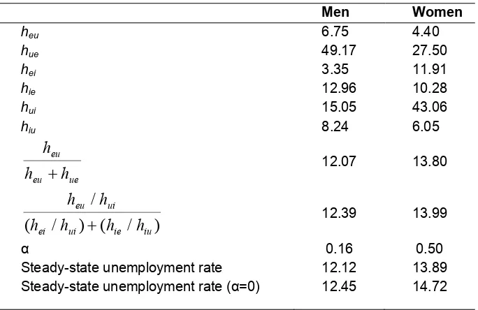
Table A6 presents the average transition probabilities between labor market states as well as the different components of the steady state unemployment rate for both men and women. The higher women’s unemployment rate is the result of their larger probability of transition from employment to inactivity (11.91% vs. 3.35%) and their lower probability of transition from unemployment to employment (27.50% vs. 49.17%).16
Looking first at the results for men, one can see that the α is small and the two components of the unemployment rate are similar. This implies that flows involving inactivity are relatively unimportant in explaining men’s unemployment rate. In the case of women, the weight α is higher. However, since the two components of the unemployment rate are also quite similar, ignoring flows involving inactivity will not lead to seriously misleading conclusions. These results do not suggest that flows involving inactivity are irrelevant to explain gender gaps in unemployment rates, but that, for some reason, they are similar to direct flows between employment and unemployment (see Azmat et al., 2006). In fact, as seen in the last two rows of Table A6, male and female unemployment rates computed according to equation (8) are very similar to unemployment rates calculated using the formula that ignores flows involving inactivity.
In view of the evidence presented above, in what follows I focus on the analyses of the flows from unemployment to employment.17 Table A7 presents
the results from pooled data estimations of a duration model for the probability of transition from unemployment to employment. The first two columns report the estimates of the hazard rate from unemployment when only the duration and gender variables are included in the model. The coefficient of the female dummy is negative, which implies that women have lower hazard rates from unemployment than men. The next two columns show the estimates that result from including individual, household and economy-wide characteristics as additional explanatory variables. According to these results, women’s hazard
16 These results are similar to those obtained by Pessino and Andrés (2000).
rate from unemployment is 10% lower than men’s.18 The last two columns
report the results when some characteristics of the last job, in particular the sector of activity, are also included in the model. The inclusion of these variables does not alter the value of the coefficient of the female dummy significantly. Figure B2 depicts the predicted hazard rates from unemployment for the representative men and women.19
The estimates that result from taking into account unobserved heterogeneity between individuals are similar to the ones presented in Table A7, so they have been omitted. The likelihood ratio test suggests that in this context unobserved heterogeneity does not significantly affect exit rates from unemployment.
To disentangle whether the differences in the hazard rates from unemployment of men and women are associated with differences in characteristics or with differences in the returns to these characteristics I estimate the previous model separately for men and women. The results are presented in Table A8. From these estimates, I decompose the gender gap in the average hazard rate from unemployment using again the methodology presented in Section III. The results of such decomposition are reported in Table A9 where we see that the gender gap in the average hazard rate from unemployment is explained almost exclusively by differences in the effects of men’s and women’s characteristics. In particular, differences in the effects of household income and marital status explain a significant part of the gender gap.
C. Interpretation of the results
In the above paragraphs, I have shown that women’s unemployment rate is higher than men’s mainly because of differences in the effects of their characteristics. Those effects are likely to be affected by two factors: (i) workers’ own attitudes, and (ii) employers’ attitudes. In this subsection, I analyze these factors in a very simple way in order to get some idea of their importance.
18 The percentage change in a hazard rate as a result of a dichotomic variable is given by 100*[1-exp(β)], where β is the coefficient associated to the dummy variable.
On the one hand, given their traditional domestic responsibilities, it is possible that unemployed women dedicate fewer resources to job search and have higher reservation wages than unemployed men. A way to consider the first hypothesis is to analyze job search intensity for both groups. In order to do this, I use the Unemployed Annex of the survey where unemployed workers report the types of job search methods they use. Table A10 presents these data for men and women. They report using the same number of job search methods and its distribution by type is very similar. Hence, the evidence presented here indicates that unemployed women devote roughly the same efforts to job search than unemployed men. The second hypothesis, referred to the minimum acceptable wage, is more difficult to contrast empirically, since the survey, as most household surveys, does not contain this information as it is not an easy measurable variable.
On the other hand, there are reasons to believe that when it comes to filling a vacancy, employers tend to favour men against women. First, it is often argued that employers prefer to hire men because hiring is costly and men are less likely to leave their jobs voluntarily. However, this hypothesis lacks sense in a country like Argentina where firing costs are high and where we would expect employers to favour those groups with larger voluntary exit rates, as women.
Second, it is usually claimed that maternity, lactation and child-care costs discourage employers from hiring women. In their study for the ILO, Berger and Szretter (2002) knock down the old myth that in Argentina employing a woman is considerably more expensive than employing a man. According to this study, the additional cost of employing a woman in firms is equal to 1% of the monthly gross wage. The main reason why these costs are so low is that monetary benefits that women workers receive during maternity leave are not paid by the employers but by social security.20
The third and last hypothesis refers to employers’ prejudices against women. The fact that the gender gap in unemployment rates is neither explained by the different characteristics of men and women nor by the existence of unobserved heterogeneity seems to point in this direction. To get some idea of the importance of gender discrimination in the Argentinean labor market I use the 1995 and 2004 Latinobarometer opinion survey. In 1995 it
asked respondents whether they believed Argentinean women have the same opportunities to get a good job as Argentinean men. Only 52% of a total of 1200 respondents answered affirmatively21. In 2004 it also asked respondents
whether they agree with the statement “Is it better that woman focuses on housekeeping and man on work?”. A 37% of respondents answered to agree with the above statement.22 Moreover, it is probable that these percentages are
higher among men than among women. Since approximately 80% of the employers are males, the discrimination hypothesis cannot be disregarded as at least partially responsible for the gender gap in unemployment rates. This would also explain the observed fact that the gender gap in unemployment rates increases with the aggregate level of the unemployment rate (see Figure B1). When the overall unemployment rate is low, as in the early 1990s, there are few applicants for most jobs, which makes it difficult for employers to discriminate against women. However, when the overall unemployment rate is high, as later in the 1990s, there are many applicants for most jobs, which make it easy for employers to put into practice their prejudices.
Finally, the estimation of structural models that enable us to disentangle the effect of the explanatory variables on the probability of receiving a job offer, related to the discrimination hypothesis, from the effect on the probability of accepting it, related to the reservation wage, will allow us to know more about the gender gap in unemployment rates. Therefore, future research in this direction could be very enlightening.
VI. Conclusions
The economic literature has dedicated little efforts to the study of the causes of the gender gap in unemployment rates. Moreover, the empirical evidence on this matter is not totally conclusive, and to a large extent refers to developed countries where the characteristics of the labor market institutions and participants are very different from those in less developed countries.
In this paper, I have studied the factors that may contribute to explain the gender gap in unemployment rates in Argentina during the second half of the
21 See 1995 press report in http://www.latinobarometro.org/. 22 See
nineties. During the 1990s, the gender gap in unemployment rates in Argentina increased noticeably, reaching more than 5 percentage points in 1996. This strong rise has spurred some concern about the underlying causes of the gender gap in unemployment rates.
Using data from the Argentinean Household Survey for the period 1995-2001, I have analyzed the factors that explain the gender gap in unemployment rates using both a static and a dynamic approach. In the first case, I estimated a random effects probit model for the probability of being unemployed. In the second case, I analyzed the flows between labor market states. Given the importance of the flows from unemployment to employment in explaining the gender gaps in unemployment rates, I estimated a duration model for the probability of leaving unemployment. Finally, in each case I carried out a decomposition analysis based on the Oaxaca-Blinder technique. Overall, I find that the gender gap in unemployment rates is explained not by differences in the observed and unobserved characteristics of men and women but by differences in the labor market returns to their characteristics. In particular, differences in the effects of household income and marital status explain a significant part of the gender gap.
References
Altonji, J. G., and R. M. Blank (1999). “Race and Gender in the Labor Market.” In Handbook of Labor Economics, ed. O. Ashenfelter, and D. Card, Vol 3C, Handbook in Economics, Vol. 5, 3143-3259. Amsterdan, North-Holland.
Arranz, J. M., J. C. Cid, and J. Muro (2000). “La Duración del Desempleo en la Argentina” [Unemployment Duration in Argentina]. Annals of AAEP.
Azmat, G., M. Güell, and A. Manning (2006). “Gender Gaps in Unemployment Rates in OECD Countries.” Journal of Labor Economics, Vol. 24 (1): 1-37.
Beblo, M, D. Beninger, A. Heinze, and F. Laisney (2003). “Methodological Issues Related to the Analysis of Gender Gaps in Employment, Earnings and Career Progression.” European Commission.
Beccaria, L. and R. Maurizio (2003). “Movilidad Ocupacional en Argentina” [Occupational Mobility in Argentina]. Annals of AAEP.
Berger, S., and H. Szretter (2002). “Costos Laborales de Hombres y Mujeres. El Caso de Argentina” [The Labor Costs of Men and Women. The Case of Argentina]. In Cuestionando un Mito: Costos Laborales de Hombres y Mujeres en América Latina [Discussing a Myth: Labor Costs of Men and Women in Latin America], ed. L. Abramo and R. Todaro. ILO, Regional Office for Latin America and the Caribbean, Lima.
Blau, F.D., P. Simpson, and D. Anderson (1998). “Continuing Progress? Trends in Occupational Segregation in the United States over the 1970s and 1980s.” Working Paper 6716, NBER.
Blau, F. D., and L. M. Kahn (2004). “The U.S. Gender Gap in the 1990s: Slowing convergence.” Working Paper 10853, NBER.
Bover, O., M. Arellano, and S. Bentolila (2002). “Unemployment Duration, Benefit Duration and the Business Cycle.” Economic Journal, Vol. 112: 223-265.
Cerimedo, F. (2004). “Duración del Desempleo y Ciclo Económico en la Argentina” [Unemployment Duration and Business Cycle in Argentina]. Working Paper no. 53, Department of Economics, Faculty of Economic Sciences, National University of La Plata.
Chamberlain, G. (1980). “Analysis of Covariance with Qualitative Data.”
Review of Economic Studies, Vol 47: 225-238.
DeBoer, L. and M. C. Seeborg (1989). “The Unemployment Rates of Men and Women: A Transition Probability Analysis.” Industrial and Labor Relations Review, Vol. 42(3): 404-414.
Dolado, J. J., F. Felgueroso, and J. F. Jimeno (2002). “Recent Trends in Occupational Segregation by Gender: A Look across the Atlantic.” Working Paper 2002-11, FEDEA.
Ehrenberg, R. G. (1980). “The Demographic Structure of Unemployment Rates and Labor Market Transition Probabilities”. In Research in Labor Economics, ed. R. G. Ehrenberg, Vol. 4. Greenwich, Conn.
Esquivel, V., and J. Paz (2003). “Differences in Wages between Men and Women in Argentina Today: Is there an Inverse Gender Wage Gap?” Annals of AAEP.
Eusamio, E. (2004). “El Diferencial de las Tasas de Paro de Hombres y Mujeres en España (1994-1998)” [The Difference between the Unemployment Rates of Men and Women in Spain (1994-1998)]. CEMFI, Thesis no. 0404. Galiani and Hopenhayn (2003). “Duration and risk of unemployment in Argentina.” Journal of Development Economics, Vol. 71(1): 199-212.
Ham, J. C., J. Svejnar, and K. Terrell (1999). “Women’s Unemployment During Transition.” Economics of Transition, Vol. 7: 47-78.
ILO (2003). “La Hora de la Igualdad en el Trabajo” [Time of Equity at Work]. Ginebra.
Jenkins, S. P. (1995). “Easy Estimation Methods for Discrete-Time Duration Models.” Oxford Bulletin of Economics and Statistics, Vol. 57: 129-138. Jenkins, S.P. (2002). Survival Analysis, ISER University of Essex, (class notes). http://www.iser.essex.ac.uk/teaching/degree/stephenj/ec968/.
Johnson, J. L. (1983). “Sex Differentials in Unemployment Rates: A Case for No Concern.” Journal of Political Economy, Vol. 91(2): 293-303.
Lauerová, J. S., and K. Terrell (2002). “Explaining Gender Differences in Unemployment with Micro Data on Flows in Post-Communist Economies.” Discussion Paper no. 600, IZA.
Mohanty, M. S. (1998). “Do U.S. Employers Discriminate Against Females When Hiring Their Employees?” Applied Economics, Vol. 30: 1471-1482. Mohanty, M. S. (2003). “An Alternative Explanation for the Equality of Male and Female Unemployment Rates in the U.S. Labor Market in the Late 1980s.” Eastern Economic Journal, Vol. 29(1): 69-92.
Mortensen, D. (1986). “Job Search and Labor Market Analysis.” In Handbook of Labor Economics, ed. O. C. Ashenfelter and R. Layard, Vol. II: 849-919. North-Holland, Amsterdam.
Mundlak, Y. (1978). “On the Pooling of Time Series and Cross Section Data.”
Econometric, Vol. 46: 69-85.
Myatt, A. and D. Murrell (1990). “The Female/Male Unemployment Rate Differential.” The Canadian Journal of Economics, Vol. 23(2): 312-322. Oaxaca, R. L. (1973). “Male-Female Differentials in Urban labor Markets”.
International Economic Review, Vol. 14: 693-709.
OECD (2002). “Women at Work: Who Are They and How Are They Faring?” Employment Outlook, 61-125. OECD.
Pessino, C. (1996). “La Anatomía del Desempleo” [La Anatomía del Desempleo]. Desarrollo Económico, Vol. 36: 223-262.
Pessino, C. and L. Andrés. (2000). “La Dinámica Laboral en el Gran Buenos Aires y sus Implicaciones para la Política Laboral y Social”[The Labor Dynamic in the Great Buenos Aires and its Implications for Labor and Social Policies]. Working Paper 173, University of CEMA.
Pessino, C. and L. Andres (2003). “Job Creation and Job Destruction in Argentina.” Inter-American Development Bank.
Petrongolo, B. (2004). “Gender Segregation in Employment Contracts.” Discussion Paper 4303, CEPR.
Saavedra, L. (2001). “Female Wage Inequality in Latin American Labor Markets.” Policy Research Working Paper Series no. 2741, World Bank. Wooldridge, J. (2002). Econometrics Analysis of Cross Section and Panel Data. MIT Press.
A. Tables
Table A1
Summary Statistics. Static Approach: Sample I
Employed Unemployed
Men Women Men Women
Personal Characteristics
Age 15-24 0.22 0.19 0.42 0.42 Age 25-34 0.32 0.31 0.24 0.28
Age 35-44 0.28 0.3 0.18 0.19
Age 45-54 0.18 0.2 0.16 0.12
Incomplete Primary Education 0.08 0.06 0.12 0.08
Complete Primary Education 0.27 0.18 0.31 0.22 Incomplete Secondary Education 0.24 0.17 0.29 0.27
Complete Secondary Education 0.21 0.22 0.16 0.21
Incomplete Tertiary Education 0.11 0.13 0.09 0.15 Complete Tertiary Education 0.09 0.23 0.03 0.08
Single 0.3 0.36 0.54 0.5
Married 0.67 0.52 0.43 0.4
Other Marital Status 0.03 0.12 0.03 0.1
Household Characteristics
Children (0-14 years) 0.67 0.62 0.6 0.66 No children 0.33 0.38 0.4 0.34 Household Income 447.45 711.67 501 602.13
Economy-wide Characteristics
Northwest 0.2 0.2 0.21 0.21
Northeast 0.13 0.13 0.11 0.09
Cuyo 0.12 0.11 0.09 0.09
Pampeana 0.27 0.28 0.33 0.34
Patagonia 0.15 0.15 0.11 0.09
Great Buenos Aires 0.13 0.13 0.16 0.18
Table A2
Summary Statistics. Dynamic Approach: Sample II
Not Censored Censored
Men Women Men Women
Duration
1-3 months 0.36 0.29 0.23 0.17
3-6 months 0.32 0.29 0.31 0.28
6 -12 months 0.22 0.25 0.27 0.28
12-24 months 0.08 0.13 0.14 0.19
More than 24 months 0.02 0.03 0.05 0.07
Personal Characteristics
Age 15-24 0.51 0.5 0.45 0.45
Age 25-34 0.25 0.29 0.21 0.26
Age 35-44 0.15 0.15 0.17 0.19
Age 45-54 0.09 0.07 0.17 0.1
Incomplete Primary Education 0.11 0.06 0.12 0.06 Complete Primary Education 0.31 0.2 0.3 0.21 Incomplete Secondary Education 0.3 0.25 0.29 0.26 Complete Secondary Education 0.16 0.21 0.18 0.24 Incomplete Tertiary Education 0.09 0.18 0.09 0.15 Complete Tertiary Education 0.03 0.1 0.03 0.09
Single 0.58 0.61 0.59 0.55
Married 0.4 0.28 0.38 0.35
Other Marital Status 0.02 0.11 0.03 0.1
Household Characteristics
Children under 14 0.64 0.65 0.58 0.66
No Children 0.36 0.35 0.42 0.34
Household Income 531 658.68 533.91 594.7
Economy-wide Characteristics
Northwest 0.18 0.2 0.21 0.21
Northeast 0.11 0.09 0.11 0.07
Cuyo 0.09 0.09 0.06 0.07
Pampeana 0.29 0.3 0.35 0.38
Patagonia 0.14 0.12 0.1 0.07
Great Buenos Aires 0.18 0.21 0.17 0.2
Last Job Characteristics
None 0.15 0.23 0.18 0.28
Agriculture 0.04 0.01 0.03 0
Manufacturing 0.41 0.09 0.39 0.1
Services 0.41 0.67 0.4 0.62
Table A3
Probability of Being Unemployed. Random Effects Probit Model. Marginal Effects. Pooled Estimations
Baseline Model Mundlak’s Correction
Marginal
Effect P-value
Marginal
Effect P-value
Personal Characteristics
Women 0.023484 0 0.024136 0
Age 15-24 0.07416 0 0.00029 0.941
Age 35-44 -0.014876 0 0.003462 0.444
Age 45-54 -0.006997 0 0.006195 0.32
Age 15-24 (Average) 0.059954 0
Age 35-44 (Average) -0.017658 0
Age 45-54 (Average) -0.011415 0.062
Incomplete Primary Education 0.032239 0 0.012486 0.001
Incomplete Secondary Education -0.000851 0.528 0.004605 0.065
Complete Secondary Education -0.028459 0 0.00589 0.077
Incomplete Tertiary Education -0.029594 0 0.007977 0.081
Complete Tertiary Education -0.060986 0 -0.00974 0.027
Incomplete Primary Education (Average) 0.019795 0
Incomplete Secondary Education (Average) -0.002787 0.337
Complete Secondary Education (Average) -0.042919 0
Incomplete Tertiary Education (Average) -0.042984 0
Complete Tertiary Education (Average) -0.110473 0
Single 0.057649 0 0.011793 0.03
Other Marital Status 0.026432 0 0.007976 0.284
Single (Average) 0.037941 0
Other Marital Status (Average) 0.015119 0.033
Household Characteristics
No Kids -0.007289 0 -0.000214 0.946
No Kids (Average) -0.006865 0.045
Household Income -0.000001 0.453 -0.000006 0.003
Household Income^2 (x10000) -0.000001 0 0.000001 0.03
Household Income (Average) 0.000011 0
Table A3 (continued)
Economy-wide Characteristics
1995 -0.0037 0.02 0.008749 0.006
1996 0.005497 0 0.012947 0
1998 -0.013927 0 -0.016356 0
1999 -0.003896 0.015 -0.01477 0
2000 0.016514 0 -0.009193 0.001
2001 0.034466 0 -0.003552 0.242
1995 (Average) -0.01614 0
1996 (Average) -0.011053 0.001
1998 (Average) -0.002383 0.448
1999 (Average) 0.007652 0.026
2000 (Average) 0.023833 0
2001 (Average) 0.042873 0
Northwest -0.015863 0 -0.015552 0
Northeast -0.035355 0 -0.034453 0
Cuyo -0.035645 0 -0.034824 0
Patagonia -0.038375 0 -0.037629 0
Great Buenos Aires 0.003223 0.066 0.002844 0.098
Log-Likelihood
-138,905.63
-138,394.04
No. of observations 354,194 354,194
No. of individuals 185,608 185,608
ρ 0.662737 0.002* 0.66565 0.002*
[image:31.595.120.471.226.528.2]Table A4
Probability of Being Unemployed. Random Effects Probit Model with Mundlak’s Correction. Marginal Effects. Separate Estimations by Gender
Men Women
Marginal
Effect P-value
Marginal
Effect P-value
Personal Characteristics
Age 15-24 0.000643 0.905 -0.000516 0.935
Age 35-44 0.013095 0.044 -0.008396 0.215
Age 45-54 0.030831 0.002 -0.020256 0.009
Age 15-24 (Average) 0.045928 0 0.076095 0
Age 35-44 (Average) -0.007487 0.235 -0.026109 0.001
Age 45-54 (Average) 0.007162 0.378 -0.028631 0.005
Incomplete Primary Education 0.013819 0.003 0.009877 0.161
Incomplete Secondary Education 0.003473 0.266 0.008163 0.087
Complete Secondary Education 0.005091 0.24 0.009222 0.118
Incomplete Tertiary Education 0.001804 0.762 0.017266 0.03
Complete Tertiary Education -0.013854 0.035 -0.005045 0.468
Incomplete Primary Education (Average) 0.022107 0 0.012319 0.091
Incomplete Secondary Education (Average) -0.011696 0.002 0.010163 0.05
Complete Secondary Education (Average) -0.051253 0 -0.033831 0
Incomplete Tertiary Education (Average) -0.047121 0 -0.038117 0
Complete Tertiary Education (Average) -0.110102 0 -0.110033 0
Single 0.019415 0.01 0.002197 0.799
Other Marital Status 0.000323 0.977 0.012604 0.224
Single (Average) 0.073124 0 0.002981 0.736
Other Marital Status (Average) 0.04818 0 -0.008033 0.397
Household Characteristics
No Kids -0.000058 0.989 -0.000939 0.861
No Kids (Average) -0.003887 0.394 -0.017455 0.002
Household Income -0.000009 0.001 -0.000002 0.536
Household Income^2 (x10000) 0.000001 0.024 0 0.795
Household Income (Average) 0.000017 0 -0.00001 0.006
Table A4 (continued)
Men Women
Marginal
Effect P-value
Marginal
Effect P-value
Economy-wide Characteristics
1995 0.013652 0.002 0.0017 0.73
1996 0.015923 0 0.009413 0.009
1998 -0.010381 0 -0.025281 0
1999 -0.003275 0.349 -0.029402 0
2000 0.007694 0.084 -0.028549 0
2001 0.01838 0 -0.027162 0
1995 (Average) -0.011679 0.015 -0.019404 0.001
1996 (Average) -0.005682 0.192 -0.017053 0.001
1998 (Average) -0.007647 0.075 0.006245 0.203
1999 (Average) 0.003009 0.516 0.017274 0.002
2000 (Average) 0.016065 0.001 0.037511 0
2001 (Average) 0.03641 0 0.056731 0
Northwest -0.011651 0 -0.020382 0
Northeast -0.02264 0 -0.047632 0
Cuyo -0.036115 0 -0.034042 0
Patagonia -0.032503 0 -0.045872 0
Great Buenos Aires -0.00454 0.033 0.016459 0
Log-Likelihood -79,499.39 -57,948.52
No. of observations 205,930 148,264
No. of individuals 105,498 80,110
ρ 0.618076 0.003* 0.677265 0.003*
[image:33.595.122.474.198.530.2]