Gender differences on sexual behaviour and school inputs:
Evidence from Bogota
Andrea Atencio De Le´
on
Thesis advisors: Darwin Cort´
es and Juan Miguel Gallego
Universidad del Rosario
September 5, 2013
Abstract
This thesis explores the correlation between school factors and the differentiated results on
sexual behaviour between boys and girls in Bogota. A school stratified propensity score matching was performed to match each boy of the sample with the most similar girls in individual, household
and school characteristics. A regression analysis was performed to estimate the correlation between the five school factors evaluated with four main outcomes: have had sexual intercourse, condom use
in the last sexual intercourse, incidence of teenage childbearing and age at first intercourse. Boys -in relation to girls - beg-in earlier their sexual life, more of them reported have used condom -in their
last sexual intercourse and have a lower incidence of teenage childbearing. These differences are correlated with have reported the school as main source of knowledge about reproductive health
and contraceptive methods, a larger proportion of teachers with a graduate or postgraduate degree, a larger proportion of teachers with a related pedagogy degree and to the average age of teachers
in the school. The results suggest that the content of the message about sex that is delivered
to girls at school is not complete or accurate and that the competences of the school teachers in charge of this task should be improved to reach equally boys and girls.
1
Introduction
have found that more highly-educated american women are less likely to engage in riskier sex-related behaviours such as unprotected sex.
Nonetheless, the positive correlation between education and safer sexual behaviour seems not affect boys and girls equally. This idea is supported by some studies that have shown that there is a gender gap in sexual behaviour and in most cases is in advantage to boys which means that, compared to girls, they have more secure sexual intercourses. For US, Cawley and Ruhm (2012) and Biswas and Vaughn (2011) found that girls reported higher likelihood of diagnosis with sexually transmitted diseases than boys; Christiansson (2006) findings suggest that males use condoms more often than females. With samples of unmarried adolescents in three Asian cities, Zuo et al. (2012) show that half of sexually active youth girls rarely or never used condoms and boys were more permissive about premarital sex. For Colombia, Atencio et al. (2013) find evidence indicating that schooled boys and girls differ in sexual behaviour outcomes, being girls who exhibit a riskier sexual behaviour1.
In spite of the demonstrated correlation between education and sexual behaviour which differ for boys and girls, research on the factors behind both, the relationship between education and safer sex-related behaviours and on gender differences with respect to risky sexual behaviour is limited. Given this, the objective of this thesis is to identify school factors, related to sex education and teachers’ characteristics, that could be correlated to sexual behaviour differences between boys and girls aged 14 to 19 years old. In particular, five school factors will be tested: school reported as main source of knowledge about reproductive health and contraceptive methods, male teachers per female teacher, average age of teachers, proportion of teachers with a graduate or postgraduate degree and proportion of teachers with a related pedagogy degree.
Many medical studies address the health consequences of risky sexual behaviour in adolescents and some of them explore the family structure and the socio-economic level as determinants to this problem (Brent, 2002; Jordahl and Lohman, 2009; Han and Waldfogel, 2007). However, to the best of my knowledge no study has explored the gender differences in sexual behaviour and the school factors correlated with these differences.
The concern for adolescents’ sexual behaviour is not only important in relation to the multiple individual effects but also related to broader implications at the national level. An empirical work conducted by the World Bank on Latin American and Caribbean countries estimates the social cost of risky youth behaviour - which includes adolescent pregnancy - equal to 2 percent of GDP annually (Cunningham et al. 2008). Maynard (1995), Moore (1978) and Eloundou-Enyegue and Stokes (2004) show that teenage childbearing may impose costs on the society since these parents spend more time on welfare programs. Fl´orez et al. (2004) and Barrera and Jaramillo (2004) show that Colombia presents a negative relation between teenage childbearing and human capital of mothers. This result is also supported by Miller (2010) who shows that access to modern family planning methods at young ages implied increasing investments in human capital and substantial socio-economic gains.
According to Chaaban and Cunningham (2011) the problem of risky youth sexual behaviour is more serious if we consider that all the studies underestimate the cost of teenage pregnancy and childbearing by not taking into account costs or consequences beyond the mothers lost productivity in the labor market, which could have implications for the children’s future productivity2, health expenditures on the mother and the social costs of single adolescent mothers. Therefore, the social inclusion of adolescent girls that keeps them on a path to achieving their maximum human potential
1
The data used to conduct the studies mentioned in this paragraph corresponds to countries that do not present a gender gap in school attendance according to the World Development Report 2011.
2
will result in significant economic growth according to this author.
United Nations Population Fund (2012) shows that Colombia presents high levels of teenage pregnancy rates compared to other Latin American countries. According to the 2010 DHS survey3, 20% of the Colombian girls aged 15 to 19 years old have been pregnant, while in other Latin American countries as Peru and Bolivia this proportion amounts to 14% and 18%, respectively. Chile and Brazil present the lowest rate of teenage pregnancy of the region with an average rate of 6% (UNPF, 2012). In developed countries this proportion is even lower amounting to 3% on average. The Colombian situation is more worrisome since 93% of women between 14 and 23 years old have received sex education at school while only half of them report to use condom at the first intercourse.
Many policies have been implemented to promote desirable sexual behaviour. These are mainly focused on reducing teenage childbearing and increasing the use of contraceptive methods. It is widely accepted that sex education is crucial for these tasks. Nevertheless, Atencio et al. (2013) find some evidence that suggests that girls and boys differ in sexual education achievement, girls know less about sex topics and present riskier sexual behaviour. The efficacy of interventions designed to reduce unin-tended pregnancy and sexually transmitted diseases among adolescents may be increased by identifying what is correlated with these gender differences.
To assess the correlation between school factors and girls’ and boys’ sexual behaviour outcomes a school stratified matching is performed in order to guarantee the comparability between boys and girls in the sample. Then, a weighted regression analysis is done showing that, in effect, the school factors evaluated are correlated with boys’ and girls’ sex behaviour and that these correlations differ between these two groups in disadvantage to girls in most of the cases, i.e., none or negative correlations with condom use and with teenage childbearing, and positive(negative) correlations with age at first sexual intercourse (have had sexual intercourse).
The next section presents more literature related with the studied topic that explains the choice of the outcomes and the school factors evaluated in this thesis. Section 3 explains the empirical strategy used to achieve the objective. Section 4 presents the sources of the data employed and some descriptive statistics of the sample followed by the results and the conclusion.
2
School factors and sex behaviour
Education is related with safer sexual behaviour. The Colombian net secondary enrollment rate for girls was 77.2% in 2010, while for boys the same indicator was 71.7%4meaning that schools are an excellent place to promote practices to improve sexual and reproductive health since most of the adolescent population is enrolled. Colombia has achieved gender equality in education and still a gender gap in sexual behaviour between girls and boys is observed meaning that the positive correlation between education an safer sexual behaviour, documented by the literature mentioned in the previous section, is not the same for these two groups. It is interesting to know which school factors are correlated with the differences in sex-related outcomes between boys and girls to improve the positive correlation between education and safer sexual behaviour in both groups, since failing to reach one of these favors the prevalence of the consequences associated with risky sexual behaviour.
When talking about the relation between sex-related outcomes and school factors, the first
3
DHS stands forDemographic and Health Survey(National Survey of Demography and Health). Survey administered by the Colombian NGO Profamilia.
4
factor that comes to mind issex education at schoolsince this is the most direct form to influence the sexual behaviour in students and recent studies have shown that comprehensive sex education have positive implications on the sexual behaviour of adolescents, including both delaying initiation of sex and increasing condom and contraceptive use (Santelli et al., 2006; Kirby, 2008; Kohler et al., 2008; Isley et al., 2010; Duberstein and Maddow-Zimet, 2012). Therefore, this factor is evaluated in this thesis and is captured by a dummy variable which takes the value 1 if the student reported school as the main source of knowledge about sexual health and contraceptive methods and 0 otherwise. Given the Colombian context, my hypothesis behind this variable is that sex education at schools is being sexist, influenced by the old perception of the roles that each gender must assume regarding sexuality and focused on biological aspects, leading to a gender gap in sexual behaviour in advantage to boys. This depends largely on the characteristics of people responsible for providing sex education, teachers. Therefore, the other school factors evaluated correspond to teachers’ features.
Student-teacher relationships may buffer adolescents from engaging in risky behaviour. It could be that students who feel connected to significant others have a sense of belonging that protects them from reaching out to other sources of comfort that may involve negative behaviour (Moritz et al., 2010). In this sense, two factors that are related with the quality of the teacher-student relationship are assessed: male teachers per female teachersratio andaverage age of teachers in the school.
On one hand one could think that the younger the teacher the better relationship with the students, leading to a smaller gender gap in sexual behaviour. However, an aged teacher could recognize better the importance of teaching and talking about sex with the students and therefore he/she takes this task more seriously. I evaluated which of these effects predominates.
On the other hand, the gender gap in sexual behaviours could be correlated with a large propor-tion of male teachers per female teacher through a low quality female student-male teacher relapropor-tionship that increases the differences between boys and girls in sex-related outcomes.
Another important characteristic of the teachers in the school that could be related with sex-related outcomes in their students is their level and kind of human capital. A greater human capital can lead to recognize the importance of a comprehensive education and hence encourage students to continue on the path to achieve their maximum human potential and stay away of risky behaviours, or simply more educated teachers teach better sex education. This factor is evaluated with theproportion of teachers with a graduate or postgraduate degreeat each school.
Regarding the ”kind” of human capital accumulated by the teachers, it is important to recognize that teaching about sex and contraceptive methods to influence sexual behaviours not only requires knowledge about the topic but awareness of the wider contexts within these issues occur. It also requires that teachers challenge traditional teaching and learning practices, which impede both critical thinking and change (Smith et.al, 2007). Therefore, theproportion of teachers with a related pedagogy degree in the school is evaluated as a school factor since a person that has been educated to teach is presumably more prepared to face the challenges that this implies: affect the lesson material, class discussions, teaching and learning methods in new and different ways and the ability to design methods that facilitate learning for both boys and girls through the recognition of the context in which they are. Knowledge of different learning styles may help to avoid that the message not be received by some group (Dunn and Griggs, 1995; Lovelace and Kiely, 2005).
An early onset of sexual activity increases the risk of negative adolescent health outcomes and theoretically, abstinence is the only way of being fully protected against Sexually Transmitted Diseases (STD). For this reason, these two outcomes are widely used by the literature to measure the effectiveness of sex education and they are indicators of sexual and reproductive health (Santelli et al., 2006; Kohler et al., 2008; Duberstein and Maddow-Zimet, 2012; Zuo, 2012; Vargas et al., 2013). Therefore,age at first sexual intercourseandhave had sexual intercourseare included as outcomes of this study and they are captured by a categorical variable that can take values from 11 to 17 indicating the interviewed age at first sexual intercourse, and by a dichotomous variable that takes the value 1 if the interviewed has had sexual intercourse and 0 otherwise, respectively.
The use of modern contraceptive methods is a sexual practice that helps to avoid non-desirable consequences on the reproductive and sexual health status of an individual. Among the contraceptive methods, the condom is the one that receives the most attention as an indicator of risky sexual behaviour in the existing literature since this method allows the prevention of two situations: pregnancy and acquiring a STD, while the other contraceptive methods just prevent the first. Therefore, the correlation for boys and girls between the aforementioned school factors and condom use in the last intercourse was estimated in this study. This outcome is a binary variable that takes the value 1 if the interviewed student5 indicated that used a condom in the last intercourse and 0 otherwise. No correlation between a given school factor andcondom use in the last intercoursefor some group (girls or boys) could be found and in that case one would be interested in knowing if there is a substitution effect between condom and other more sophisticated contraceptive methods given that the factors evaluated are related to education. To capture this, two secondary outcomes are included: modern methods
and pill, both variables are dichotomous, the first one takes the value 1 if the interviewed student indicated that he/she used at least one of the following contraceptive methods in the last intercourse: contraceptive pill, injectable method, implant or intrauterine device; and the second one, takes the value 1 if the interviewed student indicated that he/she used a contraceptive pill as contraceptive method in the last intercourse and 0 otherwise.
Teenage childbearing is a main indicator of reproductive and sexual health and it is related with the fifth Millennium Development Goal6. Teenage childbearing is one of the most studied variables in the literature related to consequences of a risky sexual behaviour since, as was mentioned, has important implications at the individual and national level (Moore, 1978; Maynard, 1995; Fl´orez et al.,2004; Barrera and Jaramillo, 2004; Cunningham et al. 2008; Fletcher and Wolfe, 2009; UNPF, 2012). For Colombia, this indicator is considered very important since teenage pregnancy has always been perceived as a negative phenomenon that should be reduced or eliminated and with this objective was born the mandatory sex education in schools, objective that was maintained for a long time and it was not satisfactorily accomplished (G´ongora, 2013). Given the importance ofteenage childbearing, it is included as a main outcome that takes the value 1 if the interviewed student or his couple is pregnant or has a child at the moment of the survey and 0 otherwise.
The literature about sexual behaviour is highly concentrated on the outcomes described above slightly leaving aside the perception that the knowledge about reproductive health and contraceptive methods could be correlated with safer sexual behaviour. Using Colombian data, Vargas et al. (2013) find that the probability of have reported sexual practices directed to improve reproductive and sexual health is greater in women with more knowledge about reproductive health and contraceptive methods.
5
In the questionnaire the information about the use of contraceptive methods is collected through the following question: The last time you had sexual intercourse, what method you or your couple used to prevent pregnancy?
6
Given this and the fact that school factors are being evaluated, knowledgeis included as a secondary outcome captured by a binary variable that takes the value 1 if the student answer correctly all the questions related to sexual and reproductive health and contraceptive methods in the questionnaire.
3
Empirical strategy
Both, a non-parametric and a parametric approach were used in the analysis.
3.1
Ensuring the comparability of the sample
The girls and boys compared must be as similar as possible in key characteristics different from gender that could affect the outcomes. This allows to estimate the gender gap in sex-related outcomes that are not explained by differences in individual, household or school variables.
To find the girls that are comparable to boys in the sample, a school stratified mahalanobis propensity score matching was used, meaning that 252 matchings were estimated, one for each school. The procedure has two steps. First, each boy (Bi = 1) in a given school is matched to the girls
(Gi = 1) in the same school with the closest propensity score. The unmatched girls and boys are
discarded. Then, the total average difference across gender (TAD) is calculated as the weighted sum of the difference in means of the outcome between boys and girls within schools. As weights, the proportion of boys in each school was used (see Dehejia and Wahba 1999, 2002). Formally,
T AD= 252
X
s=1
bs
b {[E(Yb,s)−E(Yg,s)]}
E(Yb,s)−E(Yg,s) =
1 #(bs∈CSs)
X
b,g∈CSs
{Yb,s−Yg,s}
Yg,s= X
g∈C0(X b)
WbgYg
wherebsis the number of boys in the school sandbis the number of boys in the sample7. Yb,s
and Yg,s is the sex behaviour outcome (see Table 1) of the boy b or the girl g, respectively, in the
schools. CSsis the common support of the schools- the girls and boys matched -. C0(Xb) is the set
of girls that were matched to the boyb. Wbgis the based mahalanobis distance weight on the girlg in
forming a comparison with the boyb.
Using a school stratified matching has important advantages. Variation between and within schools is taken into account, possible unobservable school and family variables that could affect the outcomes are considered - as the importance given to the education of children at home and the teachers’ endeavor in their labor - and according to Dehejia and Wahba (1999) the result obtained is very similar to that obtained from a randomized sample.
In the first part of the matching described above, individual and household characteristics such as age, grade, time of exposure (experience from now on), live with the father, live with the mother, number of children of the mother, age of the mother when she had her first child and socio-economic
7
level8 were used as covariates. The inclusion of these covariates is supported by the literature on the risk and protective factors associated with risky and sex related outcomes in adolescents and young adults (Miller, 2002; Jordahl and Lohman, 2009; Fl´orez and Soto, 2013).
It is important to stand out that the matching method was used only with the purpose of guaranteeing the comparability of the sample, i.e, find the girls that are as similar as possible to the boys with respect to household, individual and school characteristics. The matching approach has already been used to study gender gaps in other outcomes as wages ( ˜Nopo et al., 2008, 2009, 2010). However, the methodology proposed for this thesis differs from those used by ˜Nopo et al. (2009, 2010) - one to one matching - since this thesis seeks to study the average sexual behaviour difference across gender and do not intends to recover all the distribution of it. The objective of this paper is to identify what school factors could be correlated with differentiated sex behaviour between boys and girls.
3.2
Exploring the school factors
To identify the correlation between the school factors evaluated and the selected outcomes for boys and girls, a weighted regression analysis was conducted with the resulting sample from the former step. Again, the weight for each observation is the product between the school weight provided by the matching and the proportion of boys in the school. By doing this, differences between schools are taken into account and it allows for intra school variation as well. The equation to estimate is:
Yis=Gis+Bis+ (δXis+θ0Fs)×Gis+ (βXis+θ1Fs)×Bis+µis
where Yis is a sex behaviour outcome of the individual i in the school s. As mentioned, four
main outcomes were evaluated, - have had sexual intercourse, the use of condom in the last intercourse, teenage childbearing and age at first intercourse - as well as three secondary outcomes. Bisis a dummy
that takes the value one if the unit iis a boy and zero if is a girl; Gistakes the value one if the unit
i is a girl and zero if is a boy, as mentioned. Fs is the factor of schoolsevaluated (see Table 1). Xis
is the vector of covariates. The parameters of interest are θ0 and θ1 which indicates the correlation between the school factor evaluated and the outcomes for girls and boys, respectively.
Heterogeneous effects between public and private schools are considered since private schools have certain manoeuvre margin which includes sex education.
3.3
Challenges
The empirical strategy described in this section has two main challenges. First, for the analysis of some of the outcomes the sample is naturally restricted to those that have already had their first sexual intercourse, and taking this decision could be related with unobservable variables in which the compared individuals could differ generating a selection bias. Second, school reported as the main source of knowledge about reproductive health and contraceptive methods could be an endogenous variable since schools with riskier adolescents could decide to provide better sex education, this generates biased estimators of the correlation between this factor and the outcomes studied.
The first challenge arises if we assume that the cost of initiate sexual life differs between boys and girls being higher for the girls since they face the risk of getting pregnant. Therefore, one could think that the girls that have had their first sexual intercourse are less risk averse than the boys in the
8
same situation and this may be correlated with girls’ riskier sexual behaviour generating a difference in the studied outcomes which in principle the econometric exercise is not controlling for.
Related to this aspect, it is worth to mention that Bogota has the policy named”Por la calidad de la vida de ni˜nos, ni˜nas y adolescentes”. This program seeks to improve well-being of boys, girls and adolescents, as its name indicates, and teenage pregnancy is seen as one of the conditions that reduces the well-being of this population group. When an adolescent is pregnant this program provides her medical care, general information about pregnancy and baby care, food subsidy once the baby is born, and the school must monitor her health condition and family environment and send this information to the District Education Secretary (SED).
Bogota also has a District Decree (482 of 2006) establishing that technical education must be ensured to vulnerable adolescents and young adults, group in which are included adolescent mothers. Besides, at the national level to exclude or to discriminate a pregnant adolescent from the educational system is against four fundamental rights, this has been record in several sentences related to this topic9.
This institutional framework shows us that the pregnant adolescents and adolescent mothers are protected, especially in Bogota. This protection reduces the cost of getting pregnant allowing that more risk averse girls initiate their sexual lives reducing or even vanishing the possible gap in risk aversion between boys and girls that already had have a sexual intercourse in the sample used for this thesis. Moreover, if there were a gender gap in risk aversion, it should be in advantage to girls since several studies have shown that female individuals are less risk-taking that their male counterpart.
Byrnes et al. (1999) made a meta-analysis of 150 studies showing that the average effects for 14 out of 16 types of risk-taking were significantly larger for male participants than for female participants and that in certain topics, as intellectual risk-taking and physical skills, these differences are higher. The authors also show that the gender gap in risk aversion change significantly when comparing different age groups. The experimental economic literature has also robustly found that men are more risk-taking than women in the vast majority of environments, some of the studies in this field find that the gender gap in risk-taking is reduced by experience and profession (Charness, 2012; Croson, 2008). C´ardenas et al. (2012) find the same result for children aged 9-12 in Colombia and Sweden, boys in both countries are more risk taking than girls, with a smaller gender gap in Sweden. These findings on gender gap in risk behaviour suggest that when measuring gender gaps in outcomes that are related with risk-taking without controlling for it, this gap is going to be biased, boys are going to exhibit riskier behaviour than girls. For this study, this means that the differences observed in the data could be a lower bound of the real situation, boys are more risk-taking according to the literature and still they present a safer sexual behaviour.
Empirically, this issue is tackled in two different forms: the first one is controlling by charac-teristics that the literature has recognized to be highly correlated with an individual risk aversion. The second one is performing a Heckman model which corrects selection problems, model that will be intuitively explained in Section 5.1. Let me mention some of the literature referred above. Us-ing cross-section data Cohn et al. (1975) find a strong pattern of decreasUs-ing relative risk aversion, result that have been extensively reinforced by empirical and theoretical studies, and for non-wealth variables such as age, marital status, and family size, they show that inclusion or exclusion of these variables does not alter the pattern of decreasing relative risk aversion. Friend and Blume (1975) show that when human capital is incorporated into net worth, moderate increasing risk aversion is found.
9
Roger and Fernandez (1983) also found evidence supporting decreasing relative risk aversion and they show that risk aversion increases uniformly with age. Hence, for this study it is crucial to control by experience, socio-economic level, education and age.
The second challenge is tackled by trying to understand the direction of the possible bias in the estimators of the correlation between have had reported the school as main source of knowledge and the outcomes studied. This is done by comparing the adolescents that reported the school as the main source of knowledge about reproductive health and contraceptive methods and the ones that did not in the sample used for the econometric exercises described in section 3.2. This comparison is done conditioning and not conditioning on have had sexual intercourse and controlling by the school at which the student attend. In this point, it is important to mention that sex education in schools is mandatory since 1994 and there is a established guideline of what should be taught and the methodologies to do it. This was done through the Resolution No. 3353 of 1993 of the Ministry of Education. The Resolution became effective in 1994, year in which its guidelines are included in the General Law of Education. It is important to know this because through the inclusion of sex education in a law, it became a State policy that goes beyond the presidential periods and it appeared thanks to a judicial act and not a legislative act.
4
Data and descriptive statistics
To construct the database to carry out the study, three different sources of information were used: the ECSAE10, the C600 survey, and the R166 record. The institution and headquarter code assigned to each school by the National Administrative Department of Statistics (DANE) was used to merge the data.
The C600 is an annual statistical census addressed to all schools in Colombia that offer all the school levels (pre-school, elementary, middle and high school). This database is administered by the DANE and it contains general information about the school, its teachers and its students.
The R166 is a record administered by the Ministry of Education and also contains general information about the schools and detailed information about its teachers.
The ECSAE survey was designed and implemented by a team from the Universidad del Rosario with funds from PEP-BID-GRADE on the Teenage Childbearing Initiative in Latin America and the Caribbean and contains information about 38904 adolescents between 14th to 19th years old enrolled in 277 public and private schools in Bogota at the 9th, 10th and 11th grades11. The survey is repre-sentative at the locality12 and city level and it includes information about socio-economic conditions, household structure and environment, sexual behaviour, pregnancy, childbearing and knowledge/use of contraceptive methods of the interviewed students. The ECSAE survey is crucial for this study because it allows to compare sexual behaviour across gender, feature that to the best of my knowledge no other survey of a developing country contains.
Given the objective of this thesis, its empirical strategy and the sample design of the ECSAE survey13, the information used corresponds to girls and boys that are enrolled in mixed schools. Hence,
10
ECSAE stands for Encuesta sobre el Comportamiento Sexual de Adolescentes Escolarizados en Bogot´a (Survey About Sexual Behavior of Schooled Adolescents in Bogot´a).
11
In Colombia these are the final grades for completing school 12
Bogota is divided geographically and administratively in 20 localities. Each locality has several neighbourhoods and its own government which is subject to the main city government.
13
the database that was used for the econometric analysis has information about 32525 schooled adoles-cents enrolled in 252 public and private schools in Bogota.
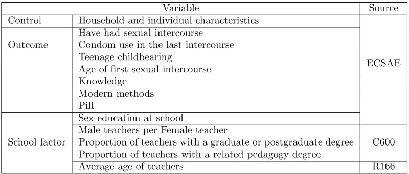
[image:10.612.92.492.135.306.2]Table 1 shows the source of the outcomes and school factors evaluated.
Table 1: Variables and sources
Variable Source
Control Household and individual characteristics
ECSAE Outcome
Have had sexual intercourse Condom use in the last intercourse Teenage childbearing
Age of first sexual intercourse Knowledge
Modern methods Pill
School factor
Sex education at school
Male teachers per Female teacher
C600 Proportion of teachers with a graduate or postgraduate degree
Proportion of teachers with a related pedagogy degree
Average age of teachers R166
4.1
Descriptive statistics
[image:10.612.158.429.462.661.2]Table 2 reports the gender distribution in the sample, before and after matching, by age. Before matching the 52.47% of the sample corresponds to girls; and approximately, one third of the sample is 15 years old. In the matched sample, 59.02% of the observations are girls and 34.5% of the adolescents is 15 years old. Given the empirical strategy employed it is important to mention that in average, 47.93% of the adolescents in each school are boys.
Table 2: Gender distribution in the sample
Full Sample Matched Sample
Age Girls Boys Total Girls Boys Total
14 N 3934 3215 7149 960 1346 2306
% 55.03 44.97 100 41.63 58.37 100
15 N 5684 4888 10572 1604 2175 3779
% 53.76 46.24 100 42.45 57.55 100
16 N 4810 4406 9216 1376 1909 3285
% 52.19 47.81 100 41.89 58.11 100
17 N 1918 2143 4061 431 776 1207
% 47.23 52.77 100 35.71 64.29 100
18 N 599 662 1261 103 219 322
% 47.50 52.50 100 31.99 68.01 100
19 N 121 145 266 10 33 43
% 45.49 54.51 100 23.26 76.74 100
Total N 17066 15459 32525 4484 6458 10942
% 47.53 52.47 100 40.98 59.02 100
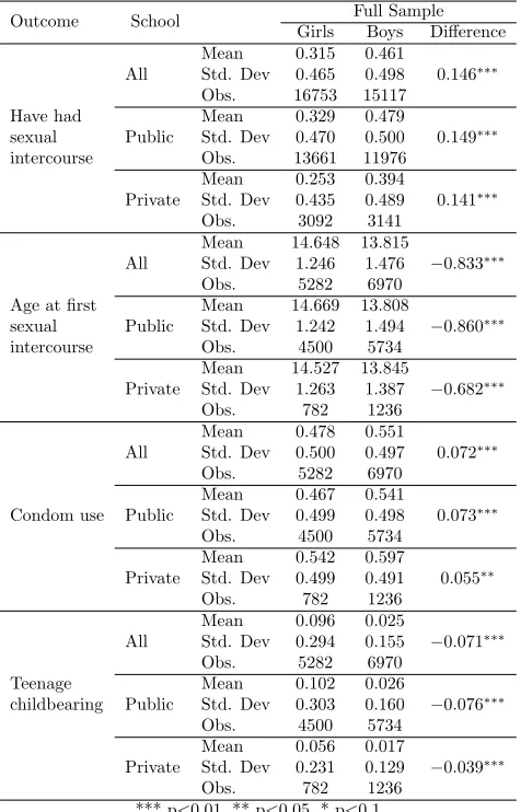
the difference of these between boys and girls in the full sample, which for the last two outcomes mentioned is naturally restricted to those that have initiated their sexual lives. The gender gap in sexual behaviour is evident, compared to girls, a greater proportion of boys reported have had sexual intercourse but also a greater proportion of boys reported have used condom in the last intercourse. Boys begin their sexual life approximately 9 months earlier than girls but these have a greater incidence of teenage childbearing, in fact, this number almost fourfold the same figure for boys. All the differences mentioned are statistically significant.
[image:11.612.174.412.326.697.2]When looking these differences for public and private schools separately, we can see that the pattern is the same for both, however, in private schools the differences are smaller but still significant. Regarding teenage childbearing, it is worth mentioning that using data from the DHS 2010, in Bogota, 16,47% of the enrolled girls aged 14-19 that had have sexual intercourse were pregnant at the moment of the interview or already had a child. The difference between this number and the same obtained from the ECSAE 2010 could be the result of differences in the sampling design. For example, the information provided by the ECSAE is collected at schools while the DHS collects the information in households.
Table 3: Descriptive statistics: Outcomes
Outcome School Full Sample
Girls Boys Difference
All
Mean 0.315 0.461
0.146∗∗∗ Std. Dev 0.465 0.498
Obs. 16753 15117
Have had
Public
Mean 0.329 0.479
0.149∗∗∗
sexual Std. Dev 0.470 0.500
intercourse Obs. 13661 11976
Private
Mean 0.253 0.394
0.141∗∗∗ Std. Dev 0.435 0.489
Obs. 3092 3141
All
Mean 14.648 13.815
−0.833∗∗∗ Std. Dev 1.246 1.476
Obs. 5282 6970
Age at first
Public
Mean 14.669 13.808
−0.860∗∗∗
sexual Std. Dev 1.242 1.494
intercourse Obs. 4500 5734
Private
Mean 14.527 13.845
−0.682∗∗∗ Std. Dev 1.263 1.387
Obs. 782 1236
Condom use All
Mean 0.478 0.551
0.072∗∗∗ Std. Dev 0.500 0.497
Obs. 5282 6970
Public
Mean 0.467 0.541
0.073∗∗∗ Std. Dev 0.499 0.498
Obs. 4500 5734
Private
Mean 0.542 0.597
0.055∗∗ Std. Dev 0.499 0.491
Obs. 782 1236
All
Mean 0.096 0.025
−0.071∗∗∗ Std. Dev 0.294 0.155
Obs. 5282 6970
Teenage
Public
Mean 0.102 0.026
−0.076∗∗∗
childbearing Std. Dev 0.303 0.160
Obs. 4500 5734
Private
Mean 0.056 0.017
−0.039∗∗∗ Std. Dev 0.231 0.129
Obs. 782 1236
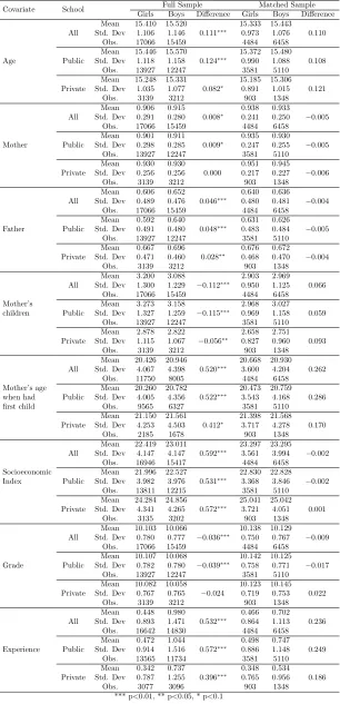
Table 4: Descriptive statistics: Covariates
Covariate School Full Sample Matched Sample
Girls Boys Difference Girls Boys Difference
Age
All
Mean 15.410 15.520
0.111∗∗∗
15.333 15.443 0.110 Std. Dev 1.106 1.146 0.973 1.076
Obs. 17066 15459 4484 6458
Public
Mean 15.446 15.570
0.124∗∗∗
15.372 15.480 0.108 Std. Dev 1.118 1.158 0.990 1.088
Obs. 13927 12247 3581 5110
Private
Mean 15.248 15.331 0.082∗
15.185 15.306 0.121 Std. Dev 1.035 1.077 0.891 1.015
Obs. 3139 3212 903 1348
Mother
All
Mean 0.906 0.915
0.008∗
0.938 0.933
−0.005 Std. Dev 0.291 0.280 0.241 0.250
Obs. 17066 15459 4484 6458
Public
Mean 0.901 0.911
0.009∗
0.935 0.930
−0.005 Std. Dev 0.298 0.285 0.247 0.255
Obs. 13927 12247 3581 5110
Private
Mean 0.930 0.930 0.000
0.951 0.945
−0.006 Std. Dev 0.256 0.256 0.217 0.227
Obs. 3139 3212 903 1348
Father
All
Mean 0.606 0.652
0.046∗∗∗
0.640 0.636
−0.004 Std. Dev 0.489 0.476 0.480 0.481
Obs. 17066 15459 4484 6458
Public
Mean 0.592 0.640
0.048∗∗∗
0.631 0.626
−0.005 Std. Dev 0.491 0.480 0.483 0.484
Obs. 13927 12247 3581 5110
Private
Mean 0.667 0.696
0.028∗∗
0.676 0.672
−0.004 Std. Dev 0.471 0.460 0.468 0.470
Obs. 3139 3212 903 1348
All
Mean 3.200 3.088
−0.112∗∗∗
2.903 2.969 0.066 Std. Dev 1.300 1.229 0.950 1.125
Obs. 17066 15459 4484 6458
Mother’s
Public
Mean 3.273 3.158
−0.115∗∗∗
2.968 3.027 0.059 children Std. Dev 1.327 1.259 0.969 1.158
Obs. 13927 12247 3581 5110
Private
Mean 2.878 2.822
−0.056∗∗
2.658 2.751 0.093 Std. Dev 1.115 1.067 0.827 0.960
Obs. 3139 3212 903 1348
All
Mean 20.426 20.946
0.520∗∗∗
20.668 20.930 0.262 Std. Dev 4.067 4.398 3.600 4.204
Obs. 11750 8005 4484 6458
Mother’s age Public
Mean 20.260 20.782
0.522∗∗∗
20.473 20.759 0.286 when had Std. Dev 4.005 4.356 3.543 4.168
first child Obs. 9565 6327 3581 5110
Private
Mean 21.150 21.561 0.412∗
21.398 21.568 0.170 Std. Dev 4.253 4.503 3.717 4.278
Obs. 2185 1678 903 1348
All
Mean 22.419 23.011
0.592∗∗∗
23.297 23.295 −0.002 Std. Dev 4.147 4.147 3.561 3.994
Obs. 16946 15417 4484 6458
Socioeconomic Public
Mean 21.996 22.527
0.531∗∗∗
22.830 22.828 −0.002 Index Std. Dev 3.982 3.976 3.368 3.846
Obs. 13811 12215 3581 5110
Private
Mean 24.284 24.856
0.572∗∗∗
25.041 25.042 0.001 Std. Dev 4.341 4.265 3.721 4.051
Obs. 3135 3202 903 1348
Grade
All
Mean 10.103 10.066
−0.036∗∗∗
10.138 10.129 −0.009 Std. Dev 0.780 0.777 0.750 0.767
Obs. 17066 15459 4484 6458
Public
Mean 10.107 10.068
−0.039∗∗∗
10.142 10.125 −0.017 Std. Dev 0.782 0.780 0.758 0.771
Obs. 13927 12247 3581 5110
Private
Mean 10.082 10.058 −0.024
10.123 10.145 0.022 Std. Dev 0.767 0.765 0.719 0.753
Obs. 3139 3212 903 1348
Experience
All
Mean 0.448 0.980
0.532∗∗∗
0.466 0.702 0.236 Std. Dev 0.893 1.471 0.864 1.113
Obs. 16642 14830 4484 6458
Public
Mean 0.472 1.044
0.572∗∗∗
0.498 0.747 0.249 Std. Dev 0.914 1.516 0.886 1.148
Obs. 13565 11734 3581 5110
Private
Mean 0.342 0.737
0.396∗∗∗
0.348 0.534 0.186 Std. Dev 0.787 1.255 0.765 0.956
Obs. 3077 3096 903 1348
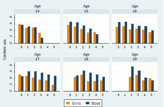
In the annex, table A1 shows descriptive statistics for have had sexual intercourse, condom use and teenage childbearing discriminated by age. It is interesting that at the only age at which the pattern shown by table 3 does not hold is 14 years old, at this age more girls reported have used condom in their last sexual intercourse than boys and this difference is statistically significant. Hence, one may think that experience plays an important role in sexual behaviour through some kind of learning process that seems to be more important to boys. Table A2 shows that this is not the case, looking at the numbers we cannot easily identify a clear pattern between experience and condom use or teenage childbearing. Nonetheless, a graph could allow us to better identify the possible trend between experience and condom use, and figure A3 suggests that given the age, the more experience the less use of condom for boys, in girls this pattern is not as clear as for boys.
Regarding the differences between boys and girls in the covariates used in the matching exercises before and after these (table 4), the result is the expected for this kind of empirical strategy. Before matching boys and girls differ in all the individual and household characteristics shown in table 4 and after matching these differences are not longer statistically significant.
In the full sample, the boys are older and have initiated their sexual life a longer time ago than the girls; the girls come from poorer households in which the father/mother is less present than in the boys’ households; boys’ mothers were older when they had their first child and had less children than mothers of the girls in the full sample.
5
Results
[image:13.612.73.504.513.619.2]To evaluate if the girls and boys in the sample are comparable after performing the matching exercises, it is necessary to check the balance property of the propensity score, if this property is fulfilled boys and girls units are observationally identical on average. The comparison of the estimated propensity scores across boys and girls provides a useful diagnostic tool to evaluate how similar are these in the matched sample, and therefore how reliable is the estimation strategy. In this sense, we expect that the density of propensity scores be the same for boys and girls, or very similar for both groups, and this is exactly what is shown in figure A2 and, in some way, in table 4.
Table 5: Naive regressions
Have had sexual intercourse
Condom use Teenage
childbearing
Age at first sexual intercourse
All −0.0131∗∗∗ 0
.0661∗∗∗ −0
.0756∗∗∗ −0
.0207∗∗∗
(0.0051) (0.0116) (0.0056) (0.0044)
Public −0.0178∗∗∗
0.0667∗∗∗
−0.0828∗∗∗
−0.0210∗∗∗
(0.0057) (0.0128) (0.0064) (0.0048)
Private 0.0062 0.0632∗∗ −0
.0399∗∗∗ −0
.0210∗
(0.0109) (0.0278) (0.0109) (0.0109)
Robust standard errors in parentheses *** p<0.01, ** p<0.05, * p<0.1
Table 5 shows the gender gap in the sex behaviour outcomes evaluated without matching boys and girls but controlling by the same covariates used on these, i.e., the gender dummy coefficient of
are statistically significant and the pattern holds when looking private and public schools separately, except for the sexual-life-initiation gap.
Table 6 shows the differences in sex behaviour outcomes between boys and girls after the match-ing exercise described in the empirical strategy section, i.e., the gender dummy coefficient of the weighted regressions. The pattern exhibited by the naive regressions holds and now the gaps are even greater, meaning that the differences in the covariates and school characteristics that are taken into account in the matching exercises are negative correlated with the gaps in sex behaviour outcomes, except for that observed in teenage childbearing.
[image:14.612.72.508.242.351.2]In general, after controlling by individual, household and school characteristics, in comparison of girls, less boys initiate their sexual life and when they do their intercourses are more secure.
Table 6: After matching
Have had sexual intercourse
Condom use Teenage
childbearing
Age at first sexual intercourse
All −0.0159∗∗ 0.0777∗∗∗ −0.0613∗∗∗ −0.0304∗∗∗
(0.0074) (0.0180) (0.0081) (0.0069)
Public −0.0225∗∗∗ 0
.0668∗∗∗ −0
.0662∗∗∗ −0
.0297∗∗∗
(0.0083) (0.0197) (0.0094) (0.0075)
Private 0.0090 0.1240∗∗∗ −0.0397∗∗∗ −0.0382∗∗
(0.0160) (0.0444) (0.0147) (0.0173)
Robust standard errors in parentheses *** p<0.01, ** p<0.05, * p<0.1
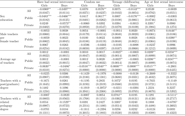
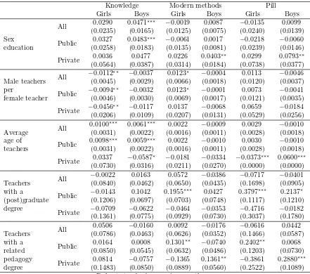
Table 7 and 8 report the correlation between each school factor and the outcomes evaluated for boys (θ1) and girls (θ0) separately.
For boys,school as the main source of knowledge about sexual health and contraceptive methodsis positively correlated with condom use and negatively correlated with incidence of teenage childbearing and the probability of have initiated sexual life; while for girls, the same factor is only correlated with the probability of have had sexual intercourse, being this correlation negative and lower than that obtained for boys. Sex education at school is not correlated with age at first sexual intercourse neither for boys nor for girls when looking all the sample.
The message delivered by sex education at schools is only well received (delivered) by (for) boys, while for girls is only effective in reducing the probability of have initiated sexual life and still is less effective than for boys in this aspect. One could think that the results on condom use could be related to a substitution effect between the condom and other contraceptive methods among girls , if this were the case, sex education at school should have a positive correlation with modern methods or withpill. However, the fifth and seventh column of table 8 do not support this idea, sex education is not correlated with the use of other modern contraceptive methods for girls (nor for boys). Moreover, the fourth column of the same table shows us that sex education is positively correlated with boys’ knowledge about sexual and reproductive health and contraceptive methods while there is no correlation for girls.
way.
The average age of teachersin the school is negatively correlated with the girls’ incidence in teenage childbearing and positively correlated with boys’ and girls’ age at first intercourse, being greater the correlation for boys (table 7). Regarding the secondary outcomes, this school factor is only correlated with girls’ and boys’ knowledge about sexual health and contraceptive methods; this correlation is greater for girls. This suggests that the effect that predominates is the second one mentioned for this factor in Section 2.2, an aged teacher may recognize better the importance of teaching and talking about sex with the students and apparently they know how to deliver the message to girls as well. They promote abstinence but also teach other sex-related topics.
Theproportion of teachers with a graduate or postgraduate degreein the school does not have a statistically significant correlation with any of the outcomes evaluated and theproportion of teachers with a related pedagogy degree does not have a ”desirable” correlation with the incidence of teenage childbearing in girls and it presents a negative correlation with boys’ age at first sexual intercourse. These results do not support the idea that more educated teachers teach better sex education and certainly the knowledge of different learning styles is not helping to avoid that the message not be received by some group at the aggregated level.
When looking the results for public and private schools separately in order to assess possible heterogeneous effects some of the patterns described above change.
Public schools
For public schools, the correlation between sex education and have had sexual intercourse is slightly greater for girls than for boys, reinforcing the idea that the only message delivered effectively to girls is abstinence.
A greater proportion of teachers with a graduate or postgraduate degree has a positive corre-lation with the girls’ incidence of teenage childbearing but also has a positive correcorre-lation with the girls’ use of modern contraceptive methods, correlation that is even greater if we only see the use of contraceptive pills. These results suggest that there is a substitution effect between the condom and other modern methods but apparently the girls are only receiving the information about the existence of these methods and not about their correct use (no correlation with knowledge). This could explain the positive correlation between the factor in mention and the girls’ incidence of teenage childbearing, since those modern methods require certain discipline in their use in order to be effective and if the girl does not know this the method is not going to work properly.
The proportion of teachers with a related pedagogy degree is negatively correlated with the boys’ probability of have initiated their sexual life, it is no longer correlated with the incidence of teenage childbearing in girls and it is also negatively correlated with boys’ age at first sexual intercourse. Although this factor does not have any correlation with the girls’ main outcomes it does have a significant correlation with girls’ use of modern contraceptive methods. For public schools, having more teachers with a related pedagogy degree seems to help to deliver a message beyond abstinence in girls, while in boys it only reduces the probability of have had sexual intercourse in some of them but in the ones that not, start their sexual life earlier. Again, the knowledge of different learning styles is not helping to avoid that the message not be received by some group, and in this case the disadvantage group is the male group.
Table 7: School factors and main outcomes
Have had sexual intercourse Condom use Teenage childbearing Age at first sexual intercourse
Girls Boys Girls Boys Girls Boys Girls Boys
All −0.0369
∗∗
−0.0497∗∗∗
0.0370 0.0576∗∗
0.0075 −0.0143∗∗∗
0.0539 −0.0039 (0.0167) (0.0114) (0.0371) (0.0237) (0.0102) (0.0054) (0.0702) (0.0551) Sex
Public −0.0483
∗∗∗ −0
.0466∗∗∗ 0
.0417 0.0617∗∗ 0
.0007 −0.0176∗∗∗ −0
.0002 −0.0303 education (0.0182) (0.0125) (0.0401) (0.0262) (0.0108) (0.0061) (0.0746) (0.0613)
Private 0.0249 −0.0573
∗∗ −0
.0060 0.0392 0.0394 −0.0013 0.3391∗ 0
.0980 (0.0402) (0.0270) (0.0959) (0.0547) (0.0279) (0.0109) (0.1984) (0.1274)
All −0.0053 0.0038 0.0054 −0.0001 −0.0014 0.0020 −0.0074 0.0446
∗∗
Male teachers (0.0060) (0.0044) (0.0179) (0.0114) (0.0048) (0.0020) (0.0361) (0.0186) per
Public −0.0059 0.0023 0.0100 0.0022 0.0009 0.0028 −0.0024 0.0390
∗∗
female teacher (0.0062) (0.0045) (0.0188) (0.0119) (0.0048) (0.0021) (0.0364) (0.0190) Private 0.0067 0.0263 −0.0596 −0.0303 −0.0195 −0.0098 −0.0237 0.0996
(0.0254) (0.0182) (0.0650) (0.0397) (0.0167) (0.0068) (0.1212) (0.0899)
All 0.0012 −0.0001 0.0010 0.0017 −0.0027
∗ −0.0003 0.0209∗∗ 0.0250∗∗∗
(0.0022) (0.0015) (0.0047) (0.0032) (0.0014) (0.0007) (0.0099) (0.0074) Average age
Public 0.0012 −0.0001 0.0012 0.0020 −0.0027
∗ −0.0003 0.0206∗∗ 0.0247∗∗∗
of teachers (0.0022) (0.0015) (0.0047) (0.0032) (0.0014) (0.0007) (0.0099) (0.0074)
Private −0.0630
∗∗
−0.0486∗
−0.0516∗∗∗
0.0340∗∗∗
0.0000∗∗∗
0.0000∗∗∗
0.0515∗∗∗
−0.2601 (0.0310) (0.0274) (0.0000) (0.0000) (0.0000) (0.0000) (0.0000) (0.6435)
All −0.0225 0.0306 −0.1429 −0.1976 −0.0088 −0.0138 −0.2689 −0.3322 (0.0907) (0.0590) (0.2180) (0.1381) (0.0680) (0.0331) (0.4832) (0.3075) Teachers with a
Public −0.1671 0.0261 −0.1195 0.2835 0.1072
∗ 0
.0195 −0.7021 −0.1149 post(graduate) (0.1645) (0.0993) (0.3193) (0.2319) (0.0560) (0.0233) (0.5721) (0.5115) degree
Private 0.1482 0.1096 −0.1919 −0.3972
∗ −0.0211 −0.0394 1.2224 0.3227
(0.1234) (0.0980) (0.3941) (0.2368) (0.0892) (0.0765) (0.8670) (0.5202)
All −0.0007 −0.0820 −0.0007 0.0054 0.0784
∗∗ 0
.0195 0.1291 −0.5111∗
Teachers with a (0.0803) (0.0563) (0.1768) (0.1151) (0.0362) (0.0131) (0.4120) (0.2717) related
Public 0.0554 −0.1529
∗∗ 0
.0391 0.2427 0.1005∗ 0
.0240 0.1888 −0.6795∗
pedagogy (0.0987) (0.0723) (0.2314) (0.1480) (0.0514) (0.0163) (0.4488) (0.3602) degree
Private −0.0701 0.0184 −0.1811 −0.2394 0.0256 0.0232 −0.0124 0.0891 (0.1311) (0.0973) (0.3015) (0.1883) (0.0530) (0.0203) (0.8388) (0.4323)
Robust standard errors in parentheses *** p<0.01, ** p<0.05, * p<0.1
Table 8: School factors and secondary outcomes
Knowledge Modern methods Pill
Girls Boys Girls Boys Girls Boys
All 0.0290 0.0471
∗∗∗ −0
.0019 0.0087 −0.0135 0.0099 (0.0235) (0.0165) (0.0125) (0.0075) (0.0240) (0.0139) Sex
Public 0.0327 0.0483
∗∗∗ −0
.0061 0.0017 −0.0218 −0.0060 education (0.0258) (0.0183) (0.0135) (0.0081) (0.0239) (0.0146)
Private 0.0036 0.0477 0.0226 0.0403
∗∗ 0
.0299 0.0793∗∗
(0.0564) (0.0387) (0.0314) (0.0184) (0.0738) (0.0377)
All −0.0112
∗∗ −0
.0037 0.0123∗ −0
.0004 0.0113 −0.0046 Male teachers (0.0045) (0.0029) (0.0066) (0.0018) (0.0120) (0.0037) per
Public −0.0094
∗∗ −0
.0032 0.0123∗ −0
.0001 0.0073 −0.0041 female teacher (0.0046) (0.0030) (0.0069) (0.0017) (0.0121) (0.0035)
Private −0.0456
∗∗ −0
.0117 0.0137 −0.0068 0.0659 −0.0184 (0.0206) (0.0109) (0.0207) (0.0131) (0.0529) (0.0256)
All 0.0100
∗∗∗
0.0061∗∗∗
0.0022 −0.0009 0.0029 −0.0010 Average (0.0031) (0.0022) (0.0016) (0.0011) (0.0028) (0.0018) age of Public 0.0098∗∗∗
0.0059∗∗∗
0.0022 −0.0010 0.0030 −0.0010 teachers (0.0031) (0.0022) (0.0016) (0.0011) (0.0028) (0.0018)
Private 0.0337 −0.0587
∗ −0
.0181 −0.0334 −0.0373∗∗∗ 0
.0600∗∗∗
(0.0730) (0.0316) (0.0211) (0.0270) (0.0000) (0.0000)
All −0.0022 0.0163 0.0572 −0.0386 −0.0717 −0.0401 Teachers (0.0840) (0.0462) (0.0650) (0.0435) (0.1698) (0.0905) with a
Public −0.0143 0.1042 0.1955
∗∗∗
0.0427 0.3797∗∗∗
0.2137∗
(post)graduate (0.1206) (0.0697) (0.0703) (0.0748) (0.1117) (0.1210) degree
Private −0.0709 −0.0622 −0.0464 −0.0353 −0.4716 −0.0182 (0.1361) (0.0775) (0.0929) (0.0730) (0.3037) (0.1780)
All 0.0506 −0.0160 0.0092 −0.0176 −0.0616 0.0442 Teachers (0.0786) (0.0463) (0.0626) (0.0352) (0.1466) (0.0587) with a
Public 0.0164 0.0008 0.1301
∗∗ −0.0740 0.2402∗∗ 0.0068
related (0.0850) (0.0545) (0.0632) (0.0486) (0.1203) (0.0730) pedagogy
Private 0.0814 −0.0757 −0.1365 0.1361
∗∗ −0.3861 0.2880∗∗∗
degree (0.1483) (0.0850) (0.0889) (0.0560) (0.2522) (0.1089) Robust standard errors in parentheses
*** p<0.01, ** p<0.05, * p<0.1
Private schools
Although the pattern of the correlations between have reported the school as the main source of knowledge about sexual health and contraceptive methods and all the outcomes evaluated is different from the described above, the conclusion is the same: the message delivered by sex education at schools is only well received (delivered) by (for) boys, but in this case for girls is only effective in increasing age at first sexual intercourse and for boys is effective in use of modern contraceptive methods. Only abstinence is promoted to girls.
Having more teachers per female teacher in a private school does not have any significant correlation with the outcomes evaluated except for girls’ knowledge about contraceptive methods and reproductive health. Correlation that remains negative.
also correlated with less use of condom and contraceptive pills. Aged teachers also promote abstinence in boys, which is reflected in the negative correlation between this factor and the probability of have had sexual intercourse. Nevertheless, for boys, this factor is also positively correlated with the use of condom and contraceptive pills (by their couple).
A greater proportion of teachers with a graduate or postgraduate degree is only correlated with boys’ condom use and not in the ”desirable” way. This negative correlation is not compensated with a positive correlation with other modern contraceptive methods. In private schools, more educated teachers do not teach better sex education or give more information about contraceptive methods as seems to happen in public schools.
A greater proportion of teachers with a related pedagogy degree is not correlated with any of the main outcomes but it is positively correlated with boys’ use of modern contraceptive methods. It is interesting that for public schools, the same correlations were found with the secondary outcomes but for girls. In both cases, the message is not received by some group.
Sex education in Colombia has always had the objective of reduce or eliminate teenage child-bearing but according to these results the way in which this goal wants to be accomplished is not being the best. Abstinence is a necessary part of sex education since it is the best way to be fully protected against pregnancy and Sexual Transmitted Diseases but it should not be provided to adolescents as a sole choice since the literature has documented the ineffectiveness of abstinence-only programs. Santelli et al., 2006; Kohler, 2008; Isley, 2010 , among others, have found that abstinence-only education did not reduce the likelihood of engaging in vaginal intercourse, it decreases reliable contraceptive method use, and it does not have a significant effect on teen pregnancy; while adolescents who received com-prehensive sex education are significantly less likely to report teen pregnancy and present a marginally lower likelihood of reporting having engaged in vaginal intercourse.
The results found by this study suggest that it is necessary to improve the information provided about modern contraceptive methods in schools, not focus the message only on abstinence or delay the first sexual intercourse and improve the competences of the school teachers providing this kind of education in order to reach equally girls and boys, since the results show that most of the school factors evaluated are correlated with desirable outcomes in boys while there is no correlation or a non-desirable correlation for girls.
5.1
Robustness checks
Table 9: Heckman Model
Benchmark Heckman Benchmark Heckman
All
Condom use 0.0777
∗∗∗ 0.1157∗∗∗ Teenage −0.0613∗∗∗ −0.0832∗∗∗
(0.0180) (0.0374) childbearing (0.0081) (0.0178)
λ 0.0255 −0.0302
(0.1405) (0.0669)
Public
Condom use 0.0668
∗∗∗ 0
.1197∗∗∗ Teenage −0
.0662∗∗∗ −0
.0916∗∗∗
(0.0197) (0.0385) childbearing (0.0094) (0.0190)
λ 0.0313 −0.0359
(0.1478) (0.0728)
Private
Condom use 0.1240
∗∗∗
0.1245∗∗∗
Teenage −0.0397∗∗∗
−0.0399∗∗∗
(0.0444) (0.0316) childbearing (0.0147) (0.0120)
λ −0.0429 −0.0160
(0.4221) (0.0213)
Standard errors in parentheses *** p<0.01, ** p<0.05, * p<0.1
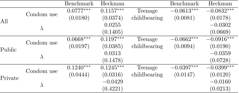
The fourth and seventh column of table 9 present the difference in condom use and teenage childbearing between boys and girls and theλcoefficient obtained from the second step of the Heckman models performed, respectively. This second step regression includes as regressors the same variables included in the benchmarck exercise plus the fitted value of the inverse Mill ratio term (λ ) which represents the estimated probability of have had sexual intercourse, probability obtained in the first step of this model. Therefore, the coefficient of this term is the correlation of interest - that between the error in the equation determining initiate or not sexual activity and the error in the equation determining condom use or teenage childbearing - to know if there is a bias due to the selection of the sample that in this case corresponds to those that have initiated their sexual life.
As we can see in table 9, the λ coefficient is statistically insignificant in all cases and low in magnitude implying that there is no selection bias in the benchmark exercise and even if there were the even rows of table 9 show us that the gender gap would be underestimated, hence, the results obtained would be a lower bound of the real problem.
It is important to mention that the probability of have had sexual intercourse, and hence of being selected, was estimated using as determinants individual and household characteristics14, and the proportion of adolescents in the same grade of the individual that had initiated their sexual lives. These variables were chosen since there is a large literature that supports that sexual initiation is highly affected by the initiation of peers, and by family and socio-economic factors (Card and Giuliano, 2012; Richards, 2012; Jordahl and Lohman, 2009; Miller, 2002; Miller et al., 2001; Upchurch et al., 1999;Billy et al., 1994). Besides, some of the individual and the socio-economic characteristics included in this first step, according to the literature, are also correlated with risk aversion as mentioned in Section 3.3, and the omission of this particular characteristic was the main concern since this could lead to a positive bias assuming that initiated girls are less risk averse than initiated boys due to a higher ”entrance cost” to sexual life.
Heckman results confirm the intuition explained in Section 3.3 about the differences in risk aversion between boys and girls that already had their first sexual intercourse in the sample used for the econometric exercises. The mentioned difference could be lower than the expected or even null
14
Table 10: Observables by gender and sex education at school conditioned on sexual activity
Covariate School Matched Sample
Girls SE Girls Difference Boys SE Boys Difference
Age
All
Mean 15.838 15.824 0.014
15.843 15.802 0.041 Std. Dev 0.953 1.011 1.084 1.083
Obs. 948 642 1619 1084
Public
Mean 15.888 15.849 0.039
15.903 15.819 0.084 Std. Dev 0.956 1.027 1.086 1.083
Obs. 768 564 1308 915
Private
Mean 15.634 15.638
−0.004
15.607 15.709
−0.102 Std. Dev 0.916 0.872 1.044 1.082
Obs. 180 78 311 169
Mother
All
Mean 0.917 0.905 0.012
0.913 0.914
−0.001 Std. Dev 0.276 0.294 0.282 0.281
Obs. 948 642 1619 1084
Public
Mean 0.919 0.903 0.016
0.912 0.907 0.005 Std. Dev 0.272 0.296 0.284 0.291
Obs. 768 564 1308 915
Private
Mean 0.907 0.919
−0.012
0.919 0.950
−0.031 Std. Dev 0.291 0.275 0.273 0.218
Obs. 180 78 311 169
Father
All
Mean 0.589 0.565 0.024
0.598 0.588 0.010 Std. Dev 0.492 0.496 0.490 0.492
Obs. 948 642 1619 1084
Public
Mean 0.581 0.563 0.018
0.593 0.583 0.010 Std. Dev 0.494 0.496 0.492 0.493
Obs. 768 564 1308 915
Private
Mean 0.622 0.579 0.043
0.620 0.620 0.000 Std. Dev 0.486 0.497 0.486 0.487
Obs. 180 78 311 169
All
Mean 3.003 3.085
−0.082
3.067 3.032 0.035 Std. Dev 0.998 1.055 1.181 1.178
Obs. 948 642 1619 1084
Mother’s
Public
Mean 3.052 3.133
−0.081
3.119 3.070 0.049 children Std. Dev 1.005 1.062 1.196 1.193
Obs. 768 564 1308 915
Private
Mean 2.804 2.733 0.071
2.863 2.819 0.044 Std. Dev 0.947 0.936 1.094 1.070
Obs. 180 78 311 169
All
Mean 20.134 19.839 0.295
20.434 20.050 0.384 Std. Dev 3.279 3.077 4.082 3.837
Obs. 948 642 1619 1084
Mother’s age
Public
Mean 19.945 19.802 0.143
20.274 19.924 0.350 when had Std. Dev 3.175 3.115 4.032 3.768
first child Obs. 768 564 1308 915
Private
Mean 20.908 20.116 0.792
21.070 20.748 0.322 Std. Dev 3.581 2.790 4.223 4.140
Obs. 180 78 311 169
All
Mean 22.731 22.666 0.065
23.041 23.163
−0.122 Std. Dev 3.650 3.585 3.952 4.022
Obs. 948 642 1619 1084
Socioeconomic Public
Mean 22.289 22.424
−0.135
22.603 22.844
−0.241 Index Std. Dev 3.403 3.468 3.775 3.979
Obs. 768 564 1308 915
Private
Mean 24.540 24.435 0.105
24.781 24.929
−0.148 Std. Dev 4.055 3.938 4.160 3.805
Obs. 180 78 311 169
Grade
All
Mean 10.365 10.298 0.067
10.293 10.199 0.094 Std. Dev 0.712 0.717 0.739 0.747
Obs. 948 642 1619 1084
Public
Mean 10.369 10.303 0.066
10.305 10.184 0.121 Std. Dev 0.711 0.721 0.744 0.752
Obs. 768 564 1308 915
Private
Mean 10.352 10.265 0.087
10.246 10.278
−0.032 Std. Dev 0.716 0.694 0.721 0.713
Obs. 180 78 311 169
Experience
All
Mean 1.320 1.383
−0.063
1.704 1.695 0.009 Std. Dev 0.967 1.009 1.121 1.174
Obs. 948 642 1619 1084
Public
Mean 1.359 1.360
−0.001
1.755 1.732 0.023 Std. Dev 0.974 1.001 1.128 1.193
Obs. 768 564 1308 915
Private
Mean 1.159 1.556
−0.397
1.501 1.495 0.006 Std. Dev 0.927 1.059 1.067 1.041
if it is taken into account that (i) the girls and boys in this sample are equal in observables highly correlated with risk aversion, condition that was achieved performing the matching exercises; and that (ii) in Bogota the institutional context favors the adolescent mother providing her medical care, health information, nutritional subsides and incentives to continue studying in order to improve her agency15 outcomes. This kind of policies combined with a legal framework that protects the right to study of the pregnant adolescents reduces the possible cost that the adolescent woman faces for starting her sexual life and even when she gets pregnant, allowing that girls with a higher risk aversion decide to initiate their sexual lives and this reduces or even vanishes the possible differences in this characteristic between initiated boys and girls.
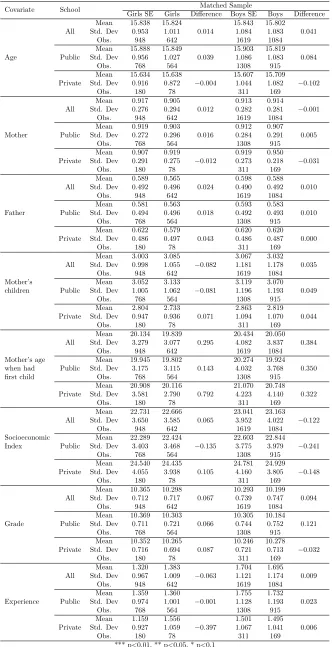
The other concern about the validity of the results is related with one of the school factors evaluated: school reported as main source of knowledge about reproductive health and contraceptive methods. One could think that the school offers better sex education as a result of riskier sexual behaviour which is traduced in bad indicators in its students, e.g. high incidence of teenage pregnancy, and in this case we would have a problem of endogeneity that leads to biased estimators. If this were the case we would like to know the direction of this bias. Hence, table 10 shows the difference in observables between those adolescents that reported the school as main source of knowledge about reproductive health and contraceptive methods (fourth and seventh column) in the matched sample with the ones that did not (fifth and octave column), this conditioned on have had sexual intercourse; in the annex, the table A3 shows the same without conditioning on sexual activity. It is important to mention that the descriptive statistics reported in these tables (10 and A3) are weighted by the same weights used in the econometric exercises, therefore, they are controlled by the school in which studies each individual.
Both, table 10 and A3 show that there are no significant differences between those girls and boys that consider the school as main source of knowledge and those that do not, therefore these two sub-samples are comparable and it should not be a bias due to this, this is reinforced by the fact that to provide sex education in schools is mandatory and schools even have certain guidelines to do this, as explained.
Given the discussed in this subsection, the results presented are straightforward and in the worst of the cases are a lower bound of the real phenomenon.
6
Conclusion
This thesis explored the correlation between scholar factors and the differentiated results on sexual behaviour between boys and girls finding that the gender gap observed in have initiated sexual life, condom use, age at first sexual intercourse and teenage childbearing incidence - measured by the number of adolescent parents and the adolescents expecting children at the moment of the survey -is correlated with have reported the school as main source of knowledge about reproductive health and contraceptive methods, a larger proportion of teachers with a graduate or postgraduate degree, a larger proportion of teachers with a related pedagogy degree and to the average age of teachers in the school.
The methodology used to achieve the objective of this study includes both a non-parametric and a parametric approach. To ensure the comparability between the boys and girls compared, a school
15