Real Time Monitoring of Railway Traffic Using Fiber Bragg Grating Sensors
8
0
0
Texto completo
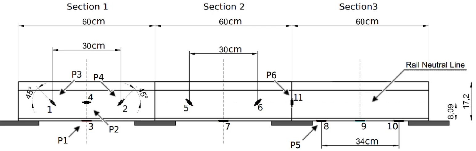
(2) This article has been accepted for publication in a future issue of this journal, but has not been fully edited. Content may change prior to final publication.. 4855-2010. 2. line because they are in good conditions and do not require usual maintenance works. The subgrade at this site is a geological formation designated as “Paramo limestone”. The traffic conditions allow recording approximately 27 train passages every day on track I, and another 27 on track II. The speeds of these trains in the measurement section are in the interval ranging between 200 and 300 km/h. The trains were primarily tested during commercial operation. The different trains tested in the experimental campaigns are described in Table I. These three train types due to their characteristics, present different values of the measurable parameters (weight per axle, number of axle, length and distance between axles). In relation to the high speed line superstructure components, the construction parameters applied have been very demanding so as to allow the development of maximum speeds of 350 kilometers per hour in commercial service (currently limited to 300 km/h) and to guarantee the interoperability of this infrastructure in accordance with European legislation. TABLE I MAIN PROPRIETIES OF THE TESTED TRAINS. TRAIN Contractor Max speed (km/h) Gauge Total length (m) Total mass (t) Number of axles Mean mass in axle (t) Distance first-last axle (m) Axles distance in wagons (m) Number of wagons. S-102 TalgoBombardier 330 UIC 200.38 322 21. S-103 SiemensVelaro 350 UIC 200.32 425 32. S-120. 250 UIC/Iberian 107.36 247 16. 17. 15. 16. 195.795. 196.81. 102.149. 13.14. 14.875. 16.2. 14. 8. 4. CAF. The tracks are laid on ballast, with a minimum thickness of 35 cm. The sleepers are of single block AI-99 type, prefabricated and made of pre-stressed concrete with the following characteristics: weight of 320 kg, length of 2600. mm, maximum base width of 300mm, and minimum height of 242 mm. The distance between sleeper axes is 0.60 m. The rail used is the 60E1 type (UIC 60) with a hardness 2607300 HBW and tensile strength larger than 880 N/mm2. The stiffness of the track must be limited in order to reduce the vertical dynamic forces between wheels and rails. This is achieved by the use of rail pads under the rail. With this aim, the pads used in this line have 7 mm thickness and a static vertical stiffness of 100 kN/mm. III. FIBER BRAGG GRATING SENSORS AND INTERROGATION UNIT FBGs are very small, short-length single-mode fiber devices that display a periodic refractive-index variation in its core [7], [9]. When a broadband light transmits through the optical fiber, the FBG written in the core reflects back a wavelength ( ) depending on the Bragg condition =2ne where ne is the effective refractive index of the core and is the grating period. The shift in the reflected wavelength B of the Bragg grating sensor is approximately linear to any applied strain or temperature (within a certain measurement range). Therefore, the detection technique used by the monitoring system is to identify this wavelength shift as a function of strain or temperature. The FBG sensors used for this application are 7 mm long with a reflectivity of more than 75% and bandwidths of 0.2 nm. Previous laboratory experiments proved that the FBGs used show a strain sensitivity of 1.2 pm/µε (maximum strain admitted ±2000 µε) and a temperature sensitivity of 10 pm/ºC. Another unusual characteristics of the FBGs used is that the reflection spectrum has a Gaussian peak profile with a side lobe suppression >10dB. In this campaign we selected six different positions of the sensors with respect to the rail. A total number of 20 FBG sensors have been installed, 10 per track (see fig. 1 for details of the disposition). Three consecutive spaces between sleepers have been selected. In the first space we put four FBG sensors: one in the middle between the two sleepers and adapted to the rail foot - this FBG sensor (P1) is working in pure flexion; a pair of them are adapted to the rail web with an angle with respect to the rail neutral line of 45º - these two FBG sensors. Fig. 1. Disposition of 10 FBG sensors along one of the rails.. Copyright (c) 2011 IEEE. Personal use is permitted. For any other purposes, Permission must be obtained from the IEEE by emailing [email protected]..
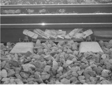
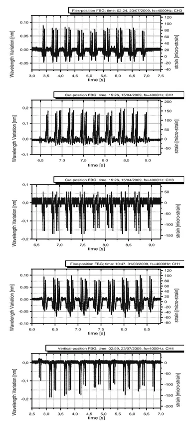
(3) This article has been accepted for publication in a future issue of this journal, but has not been fully edited. Content may change prior to final publication.. 4855-2010 (P3 and P4) are working in shear - and the last one (P2) is placed just on the rail neutral line in order to check temperature changes in the rail. In the second section between sleepers we use the same sensor structure without the temperature FBG and the third section has a vertical sensor just in the centre of the sleeper (P6) and three flexion sensors placed at different distances between the sleepers (among them, P5). The FBG sensors are directly pasted with an epoxy resin on the rail tracks. Prior to installation, the surface of the rail was polished to remove any oxide rests and ensuring that it was not get too irregular. The surface was cleaned with a tissue and alcohol. All the installation of the sensors was performed in the time period in which the current commercial service is stopped and when the usual maintenance operations allow it (from 1:00 to 4:00 AM). The typical temperature of the rail in this time period was between -5ºC and +10ºC. The temperature and the roughness of the surface did not allow to use cyanocrilate or similar glues. As a good alternative, we used a fast-curing epoxy (5 minutes) withstanding 240 kg/cm2. 30 minutes after installation, the FBG sensors were covered and protected with silicone and power tape. The final result is displayed in Fig. 2. The installed FBG sensors have been running one year without losses in their performance even after heavy snows, extremely hot summer days and conventional operations of maintenance in the track.. 3 sleepers in less than 10 ms. By using add/drop wavelengthdivision multiplexing, it also allows the measurement of four sensors connected in series, operating within predefined wavelength bands. The central wavelengths of the bands used in our experiment are: 1541.49, 1547.86, 1554.28 and 1560.75 nm. The optical interrogation unit is connected to a PXI architecture system, so it is possible to increase the number of electrical and optical switching modules in the extra slots of the rack. For the electrical acquisition, NI-PXI6040 data acquisition cards are used. A special software application running under LabView (National Instruments) was developed specifically for controlling the source and detector system and for acquiring and saving the data from each sensor. This software allows reading and storing the data in wavelength variation of the four sensors up to a sampling frequency of 8000 samples/s in each of the four sensors. The data processing is made by a PC that records the train footprint traces and converts them to relative deformation units (µε). The PC and the interrogation unit were placed in the technical building around 40 m away from the tracks. In opposition to conventional electrical sensors, the virtually transparent behavior of optical fibers allows to have the interrogation unit very far from the measured points without any degradation on the measurement performance. The FBG sensors were connected by optical cables to an optical fiber backbone that runs below tracks to the auxiliary office. In this office a PC and the demodulation unit read the sensors, store the data and display the train footprints. The passage of the trains displayed and stored with this PC can also be observed with any other computer in real time through conventional wireless communication technology. In order to trigger the measurements we do not use any extra electrical or optical signal. Our system permanently takes measurements and the storage is activated whenever a train event is detected. Only the traces which present train passing are stored. This way we can avoid the installation of additional presence sensors and solve the problem of synchronization. IV. RESULT AND DISCUSION. Fig. 2. A section between sleepers covered and protected.. The interrogation unit used in the experimental campaigns is based on the BraggSCOPE technology [10, 11], which combines a high-power broadband optical source with a thinfilm optical edge filter. The edge filter allows translating the wavelength variations into optical intensity variations, which can be easily recorded at high speed by means of a data acquisition card. Two edge filters (with positive and negative slopes) are used per Bragg wavelength, so as to ensure that the setup is self-referenced. The whole system allows a dynamic measurement of the Bragg wavelength at sampling frequencies beyond 1 kHz. These acquisition speeds are necessary in highspeed railway since the train covers the distance between. Samples of the traces detected by the sensors in positions P1, P3, P4, P5 and P6 are displayed in Fig. 3 (Bragg wavelength shift and equivalent strain versus time). The trace recorded with P2 has no relevant mechanical response under the train passage (as expected, since it is placed in the neutral line of the rail). This is a good choice then to detect the ambient temperature changes. These changes are nevertheless significant in time scales much longer than the train passage, so the information given by this sensor is not strictly necessary for the adequate determination of strain in the rail. Fig. 4 shows temperature changes recorded by these sensors throughout the first hours of the morning of a sunny day of March.. Copyright (c) 2011 IEEE. Personal use is permitted. For any other purposes, Permission must be obtained from the IEEE by emailing [email protected]..
(4) This article has been accepted for publication in a future issue of this journal, but has not been fully edited. Content may change prior to final publication.. 4855-2010. 4 Flex-position FBG; time: 02:24, 23/07/2009, fs=4000Hz; CH3. 1541,45. 120. 1541,40. 100. 40 0,00. 20 0 -20. -0,05. -40 3,0. 3,5. 4,0. 4,5. 5,0. 5,5. 6,0. 6,5. 7,0. 15. 1541,30 1541,25. 10. 1541,20 5. 1541,15 1541,10. 0. 1541,05 0. 7,5. time [s]. 1. 2. 3. time [h]. 4. 5. Temperature [ºC]. 60. Wavelength [nm]. 0,05. 20. 1541,35. 80. strain [micro-strain]. Wavelength Variation [nm]. 0,10. 6. Fig. 4. Temperature variation of the rail between 5:00 and 11:00 AM in a sunny morning of March.. Cut-position FBG; time: 15:26, 15/04/2009, fs=4000Hz; CH1. 200 0,2. 100 0,1 50 0,0. 0 -50. -0,1 6,5. 7,0. 7,5. 8,0. 8,5. strain [micro-strain]. Wavelength Variation [nm]. 150. 9,0. time [s]. Cut-position FBG; time: 15:26, 15/04/2009, fs=4000Hz; CH3. 0,1. 0,0. 0 -50. -0,1 -100 -150 -0,2 6,5. 7,0. 7,5. 8,0. 8,5. strain [micro-strain]. Wavelength Variation [nm]. 50. Each individual wheel passing through the FBG sensor is clearly identifiable. The minimum induced strain due to a wheel passing on the track is more than 140 pm - peak to peakand the noise in the determination of the Bragg wavelength is less than 10 pm, giving a SNR better than 12 dB (1.2 pm means 1 µε). These FBG sensor traces show a high immunity to electromagnetic fields. No noise coming from the catenary can be seen, in comparison with the one appearing in conventional strain gauges in Fig. 5.. 9,0. time [s]. Flex-position FBG; time: 10:47, 31/03/2009, fs=4000Hz; CH1. Time (s). 120 0,10. Fig. 5. Strain gauge sensors trace obtained at train passage. The noise close to horizontal line is due to electromagnetic interferences.. 100 60 40 20. 0,00. 0 -20. -0,05. -40 -60 -80. -0,10 6,0. 6,5. 7,0. 7,5. 8,0. strain [micro-strain]. Wavelength Variation [nm]. 80 0,05. The analysis of these traces can lead to very interesting applications in the railway domain, and in particular for highspeed systems. In the following we identify and validate several of them.. 8,5. time [s]. A. Axle counter and train type identification Axle counting is an elementary security measure in railway control. As a train passes, the number of axles is counted by 0,0 0 means of a magnetic sensor. Two of such counting units -50 determine when the train is on a section or not. In high-speed -0,1 -100 trains, magnetic brakes are used in the train vehicles. These are composed of large metal pieces mounted on the bogie of the -150 -0,2 vehicle, just a few centimeters above the track. Conventional -200 axle counters can sometimes detect these as another axle, 2,5 3,0 3,5 4,0 4,5 5,0 5,5 6,0 6,5 7,0 time [s] leading to false alarms. A way to avoid these false alarms Fig. 3 Traces (time versus wavelength variation and time versus strain) would be to use optical axle counters. Axle counting using the FBG sensing system shown above is obtained from sensors P1, P3, P4, P5 and P6 for a S103 train circulating with velocity between 250 and 300 km/h. obtained by counting the number of successive “rapid” shifts in the wavelength of the optical signal reflected by the FBG. By comparing the number of axles counted and the characteristics of the trains (Table I shows the principal differences between trains), we can also use this system to identify the type of train circulating in the network. We have employed the FBG sensing system as a regular axle counter and have never observed any miscount so far (operation over strain [micro-strain]. Wavelength Variation [nm]. Vertical-position FBG; time: 02:59, 23/07/2009, fs=4000Hz; CH4. Copyright (c) 2011 IEEE. Personal use is permitted. For any other purposes, Permission must be obtained from the IEEE by emailing [email protected]..
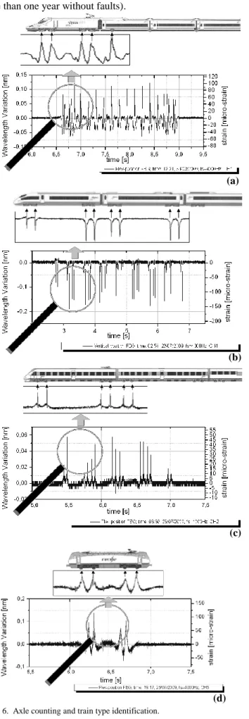
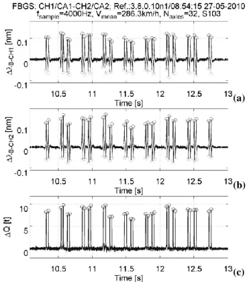
(5) This article has been accepted for publication in a future issue of this journal, but has not been fully edited. Content may change prior to final publication.. 4855-2010. 5. more than one year without faults).. Fig. 6 shows some examples of axle counting and train type identification using different sensors and different trains. In (a), we identified a S102 train (21 axles, 4 axles in the tractor head, 13 axles in 12 wagons and 4 axles in the back tractor) using sensor P1. In (b) we use the sensor P4 to identify a train type S103 (this train has distributed traction in 32 axles, 4 axles in each wagon up to a total of 8 wagons). In (c) we use a sensor in position P5 that identifies a S120 train (the traction is distributed in 16 axles, four axles per wagon). Finally in (d) we use a sensor in position P1 that identifies a maintenance locomotive running at 70 km/h.. (a). (b). (c). B. Train speed and acceleration. After having identified the train and given that the distances between the wheels are known for each specific kind of train, the train speed can be simply computed by using the trace obtained with just one FBG sensor, independently of its position in the rail. The average speed of the trains is calculated from the total distance between the first and last axle divided by the time spent between both detections. The instantaneous speed is obtained similarly using the first and the last axle but in the same wagons, so comparing the first car speed and last car speed we calculate the acceleration. Table II shows some of the results obtained. The uncertainty has been calculated using the time resolution of the acquisition system, the calibration uncertainty and mechanical tolerances [12]. An interesting result can be seen in Table II for the S-102 train. The average speed recorded is lower than the speed measured for the first and last wagon. This is because the train enters the instrumented sector decelerating but leaves the sector accelerating (the train is rather long, 200 meters as shown in table 1). Thus the average speed in the sector is smaller than the speeds recorded for the first and last wagon when they enter and leave the instrumented sector, respectively. A detailed inspection of the speeds of all the wagons passing over the instrumented sector confirms this behavior. Concerning the acceleration, in this case it should be interpreted as a “net” acceleration (the net acceleration of the train from the time in which it enters the instrumented sector and the time in which it leaves it). TABLE II TYPICAL VALUES OF THE AVERAGE AND INSTANTANEOUS SPEED OF THE DIFFERENT TRAINS AND THEIR UNCERTAINTY. Train type Average speed (km/h) Uncertainty (%) Speed of first wagon (km/h) Speed last wagon (km/h) Uncertainty (%) Sign of acceleration. S103 S102 S120 300.596 205.607 206.121 0.007% 0.007% 0.012% 300.705 208.662 204.771 300.706 207.774 206.784 0.10% 0.09% 0.07% 0 +. (d) Fig. 6. Axle counting and train type identification.. Copyright (c) 2011 IEEE. Personal use is permitted. For any other purposes, Permission must be obtained from the IEEE by emailing [email protected]..
(6) This article has been accepted for publication in a future issue of this journal, but has not been fully edited. Content may change prior to final publication.. 4855-2010. 6. C. Dynamic load monitoring. The dynamic load is an important parameter for railway infrastructure managers because excessive load in the vehicles cause degradation both in the vehicles and in the infrastructure. We have studied the dynamic load of a train passing at regular speed (between 200 and 300 km/h). In order to monitor dynamic load we use the sensors in P3 and P4 positions. These two sensors are located in the rail web with an angle of 45º with respect to the neutral line of the rail, and therefore they are intended to measure shear strain. The wavelength shift measured with these sensors is converted to strain (the conversion constant for our FBG sensors is 1.2 pm/µε). With the shear strain measured from these two sensors, one can derive the dynamic load using mechanical laws. The dynamic load (Q) is calculated with the well known equation of the elasticity theory (see [13] and [14], for instance) using the difference of the two strain traces (P3 and P4) expressed in µε through the equation 1: 2 Q xz. xz. Gb G I y. (b). (1). Sy. where Qxz is the vertical load in the centre of the rail section between sleepers, xz is the differential strain measured by substracting the strain traces of P3 and P4, G is the tangential elasticity module, bG is the width of the section in the rail neutral line, Iy the inertial momentum of the section and Sy is the static momentum of the lower part of the rail. Using the values of the UIC 60 rail we obtain: Gb G I y. (2). 0 . 17344. Sy. and so the load for each wheel is obtained as: Q xz. (a). 0 , 34688. xz. ( KN ). (3). Fig. 7 (a and b) shows the traces obtained with P3 and P4 for a S-103 train running in track I. In Fig. 7 (c) the calculated dynamic load for each wheel is depicted. In the case of Fig. 7, the dynamic load of each wheel oscillates between 7 and 9 tons, a little higher than the nominal static load defined for this train (mean mass per axle is 15 t in the S-103). This is in good agreement with the expected values.. (c) Fig. 7. Dynamic load for a S-103 train running in track I. (a & b) are the traces obtained from the shears sensors (positions P3 and P4) and (c) is the calculated dynamic load.. Fig. 8 shows the same traces for the S-120 train obtained in track II. In this case the dynamic load of each wheel oscillates between 6 and 9 t, with a mean value near or even below the static mass expected (mean mass per axle is 16 ton in S-120). The difference found between the dynamic loads measured and the static mass per axle of the train is under study. These differences could be explained by different calibration factors due to different adherence of the epoxy, or imbalance between axles. The differences in the calibration factor due to the adherence of the epoxy could be eliminated by calibration of the track sensors with a known train.. Copyright (c) 2011 IEEE. Personal use is permitted. For any other purposes, Permission must be obtained from the IEEE by emailing [email protected]..
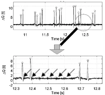
(7) This article has been accepted for publication in a future issue of this journal, but has not been fully edited. Content may change prior to final publication.. 4855-2010. 7. (a). (a). (b) (b) Fig. 9. Trace of a S-120 with flat wheel effects and detail.. (c) Fig. 8. Dynamic load for a S-120 train running in track II. (a & b) are the traces of the shears sensors (positions P3 and P4) and (c) is the calculated dynamic load.. D. Wheel imperfection detecting In high-speed railways, wear in the train wheels due to strong braking is frequent. The most evident consequence of this wear is the appearance of abnormal abrasions in the wheel thread called “flats”. Flat spots in the wheel cause strong impacts in the normally smooth power flow from the wheels to the rails. For this reason, wheel flats are a major source of problems in railway systems since they cause strong degradation both in the vehicles and in the infrastructure. Furthermore, they bring noise and discomfort to passengers and they may even cause derailments in extreme cases. The strongest and clearly visible defect in a wheel is the “plane”, a specific point of a wheel without roundness. The energy generated by a plane is strong and periodical and can be simply identified in the dynamic load trace. The repetition frequency is related to the train speed and the diameter of the wheel through the equation: f p [H z ]=. v tra in [m /s ]. (4). D [m ]. These periodical impacts are visible when the defective wheel is near the sensor but if the defect is very evident, they can also be visible relatively far from the defective wheel (through the vibrations induced in the rail). An example of plane wheel is visible in Fig. 9 (a) near t=12.5s and in detail in Fig. 9 (b). The wheel with plane is probably in t=12.4s.. V. CONCLUSION In conclusion, we have shown that fiber optic sensing technology is adequate for railway security monitoring systems. In this particular paper, we have presented a preliminary study on the use of FBG sensors for monitoring railway footprints of high speed trains (passing at speeds between 200 and 300 km/h, in the high speed line MadridBarcelona). The results illustrate that there is a consistence between the signals recorded and the wheel-rail interactions under the same operational conditions. The health of the rail, like of the wheel, can influence the deformation of the rail following the passage of the train and therefore they can both be diagnosed by analyzing and comparing the strain information measured by the FBG sensors along the time. We have demonstrated the possibility to use these sensors placed in different positions in the rail and track to know: temperature of rail, train speed and acceleration, axle counter and train type identification, dynamic load estimation and wheel defects. Further studies must be done in order to improve the dynamic load estimation results and to refine the thresholds necessary to classify a wheel as “defective”. The experience obtained from this study also highlights the potential difficulties in realizing this remote-sensing setup in practice. This is undoubtedly very useful for defining further works and seeking for improvements on both effectiveness and reliability of defect detection. REFERENCES [1]. [2].. http://www.uic.org/ Alan D. Kersey, Michael A. Davis, Heather J. Patrick, Michel LeBlanc, K. P. Koo, Member, IEEE, C. G. Askins, M. A. Putnam, and E. Joseph Friebele "Fiber Grating Sensors" JOURNAL OF LIGHTWAVE TECHNOLOGY, VOL. 15, NO. 8, AUGUST 1997.. Copyright (c) 2011 IEEE. Personal use is permitted. For any other purposes, Permission must be obtained from the IEEE by emailing [email protected]..
(8) This article has been accepted for publication in a future issue of this journal, but has not been fully edited. Content may change prior to final publication.. 4855-2010 [3].. [4].. [5].. [6].. [7].. [8]. [9]. [10]. [11]. [12].. [13]. [14].. 8. K. Y. Lee, K. K. Lee, S. L. Ho, “Exploration of Using FBG Sensor for Axle Counter in Railway Engineering,“ WSEAS Trans. on Sys., 6, 2004, pp. 2440-2447. S.L. Ho, K.Y. Lee, K.K. Lee, H.Y. Tam, W.H. Chung, S.Y. Liu, C.M. Yip and T.K. Ho, „A comprehensive condition monitoring of modern railway‟, IET Intl. Conf. on Railway Condition Monitoring, pp.125129, (2006). H.Y. TAM, S.Y. Liu, B.O. Guan, W.H. Chung, T.H.T Chan, and L.K. Cheng. “Fiber Bragg Grating Sensors for Structural and Raihvay Applications” (Invited Paper) Photonics Asia 2004, Beijing, 8·12 November 2004 T.H.T. Chan, L. Yu, H.Y. Tam, Y.Q. Ni, S.Y. Liu, W.H. Chung, L.K. Cheng. Fiber Bragg grating sensors for structural health monitoring of Tsing Ma bridge: Background and experimental observation. Engineering Structures 28 (2006) 648–659. C Barbosa, N Costa, L A Ferreira, F M Araujo, H Varum, A Costa, C Fernandes and H Rodrigues. “Weldable fibre Bragg grating sensors for steel bridge monitoring”. Meas. Sci. Technol. 19 (2008) 125305. J. Dakin and Brain Culshaw, Optical fiber Sensor: Principles and Components, Artech House, Norwood, MA, 1988 J. M. Lopez - Higuera, Ed, "Handbook of optical fiber sensing Technology," J. Wiely & Sons, USA, 2004 http://www.fibersensing.com/ Manfred Kreuzer, HBM, Darmstadt, Germany, „Strain Measurement with Fiber Bragg Grating Sensors‟. Pedro Salgado, María Luisa Hernanz-Sanjuán, Sonia Martín López y Pedro Corredera, 'Desarollo de un método de calibración de interrogadores de redes de Bragg en fibra óptica' Simposio de Metrología 2010 27 al 29 de Octubre SM2010-S3B-3. López-Pita, Andrés. Infraestructuras Ferroviarias. Ediciones UPC. Barcelona 2006. B. Glisic and D. Inaudi,2007 John Wiley & Sons, Ltd. ISBN: 978-0470-06142-8 „Fibre optic methods for structural health monitoring‟.. Massimo Leonardo Filograno Massimo L. Filograno was born in Mesagne, Italy, in January 1980. He received the "Laurea" (5 year program) degree in Electronic Engineering from the Polytechnic of Bari, Bari, Italy, in 2009, discussing a thesis with entitled "Real Time Monitoring of railway infrastructures using technology based on fiber Bragg grating". Since September 2008 till September 2010, he was with the GRIFO (Group of Photonics Engineering of the University of Alcala, Madrid) and is currently working in CSIC (the Spanish National Research Council) toward the Ph.D. degree of the Information Engineering Department, University of Alcala. His principal research interests include optical fiber sensors applied to high speed train systems.. Copyright (c) 2011 IEEE. Personal use is permitted. For any other purposes, Permission must be obtained from the IEEE by emailing [email protected]..
(9)
Figure
+3
Documento similar