Vol. 40, N 5, 2006, pp. 843–869 www.edpsciences.org/m2an DOI: 10.1051/m2an:2006036
A RESIDUAL BASED
A POSTERIORI
ERROR ESTIMATOR
FOR AN AUGMENTED MIXED FINITE ELEMENT METHOD
IN LINEAR ELASTICITY
∗Tom´
as P. Barrios
1, Gabriel N. Gatica
2, Mar´
ıa Gonz´
alez
3and Norbert Heuer
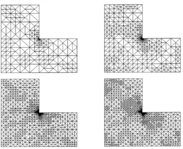
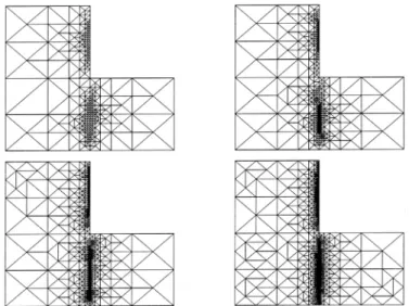
4Abstract. In this paper we develop a residual based a posteriori error analysis for an augmented mixed finite element method applied to the problem of linear elasticity in the plane. More precisely, we derive a reliable and efficienta posteriorierror estimator for the case of pure Dirichlet boundary condi-tions. In addition, several numerical experiments confirming the theoretical properties of the estimator, and illustrating the capability of the corresponding adaptive algorithm to localize the singularities and the large stress regions of the solution, are also reported.
Mathematics Subject Classification. 65N15, 65N30, 65N50, 74B05.
Received: November 9, 2005.
1.
Introduction
A new stabilized mixed finite element method for plane linear elasticity was presented and analyzed recently in [10]. The approach there is based on the introduction of suitable Galerkin least-squares terms arising from the constitutive and equilibrium equations, and from the relation defining the rotation in terms of the displacement. The resulting augmented method, which is easily generalized to 3D, can be viewed as an extension to the elasticity problem of the non-symmetric procedures utilized in [8] and [11]. It is shown in [10] that the continuous and discrete augmented formulations are well-posed, and that the latter becomes locking-free and asymptotically locking-free for Dirichlet and mixed boundary conditions, respectively. Moreover, the augmented variational formulation introduced in [10], being strongly coercive in the case of Dirichlet boundary conditions, allows the utilization of arbitrary finite element subspaces for the corresponding discrete scheme, which constitutes one of its main advantages. In particular, Raviart-Thomas spaces of lowest order for the stress tensor, piecewise linear elements for the displacement, and piecewise constants for the rotation can be used. In the case of mixed boundary conditions, the essential one (Neumann) is imposed weakly, which yields the introduction of
Keywords and phrases. Mixed finite element, augmented formulation,a posteriorierror estimator, linear elasticity.
∗ This research was partially supported by CONICYT-Chile through the FONDAP Program in Applied Mathematics, by the
Direcci´on de Investigaci´on of the Universidad de Concepci´on through the Advanced Research Groups Program, and by the Universidade da Coru˜na through the Research Grants Program.
1 Facultad de Ingenier´ıa, Universidad Cat´olica de la Sant´ısima Concepci´on, Casilla 297, Concepci´on, Chile.[email protected] 2 GI2MA, Departamento de Ingenier´ıa Matem´atica, Universidad de Concepci´on, Casilla 160-C, Concepci´on, Chile.
3 Departamento de Matem´aticas, Universidade da Coru˜na, Campus de Elvi˜na s/n, 15071 A Coru˜na, Spain.[email protected] 4BICOM and Department of Mathematical Sciences, Brunel University, Uxbridge, UB8 3PH, UK.[email protected]
c
EDP Sciences, SMAI 2007
the trace of the displacement as a suitable Lagrange multiplier. This trace is then approximated by piecewise linear elements on an independent partition of the Neumann boundary whose mesh size needs to satisfy a compatibility condition with the mesh size associated with the triangulation of the domain. Further details on the advantages of the augmented method can be found in [10] and also throughout the present paper (see, in particular, Sect. 5 below).
According to the above, and strongly motivated by the competitive character of our augmented formulation, we now feel the need of deriving correspondinga posteriorierror estimators. More precisely, the purpose of this work is to develop a residual baseda posteriori error analysis for the augmented mixed finite element scheme from [10] in the case of pure Dirichlet boundary conditions. A posteriorierror analyses of the traditional mixed finite element methods for the elasticity problem can be seen in [5] and the references therein. The rest of this paper is organized as follows. In Section 2 we recall from [10] the continuous and discrete augmented formulations of the corresponding boundary value problem, state the well-posedness of both schemes, and provide the associateda priorierror estimate. The kernel of the present work is given by Sections 3 and 4, where we develop the residual baseda posteriori error analysis. Indeed, in Section 3 we employ a suitable auxiliary problem and apply integration by parts and the local approximation properties of the Cl´ement interpolant to derive a reliable a posteriori error estimator. In other words, the method that we use to prove reliability combines a technique utilized in mixed finite element schemes with the usual procedure applied to primal finite element methods. It is important to remark that just one of these approaches by itself would not be enough in this case. In addition, up to our knowledge, this combined analysis seems to be applied here for the first time. Next, in Section 4 we make use of inverse inequalities and the localization technique based on triangle-bubble and edge-bubble functions to show that the estimator is efficient. We remark that, because of the new Galerkin least-squares terms employed, most of the residual terms defining the error indicator are new, and hence our proof of efficiency needs to previously establish more general versions of some technical lemmas concerning inverse estimates and piecewise polynomials. Finally, several numerical results confirming reliability, efficiency, and robustness of the estimator with respect to the Poisson ratio, are provided in Section 5. In addition, the capability of the corresponding adaptive algorithm to localize the singularities and the large stress regions of the solution is also illustrated here.
We end this section with some notations to be used below. Given any Hilbert spaceU,U2andU2×2denote, respectively, the space of vectors and square matrices of order 2 with entries inU. In addition,Iis the identity matrix ofR2×2, and givenτ := (τij),ζ:= (ζij)∈R2×2, we write as usual
τt
:= (τji), tr(τ) := 2
i=1
τii, τd:=τ−1
2tr(τ)I, and τ :ζ := 2
i,j=1 τijζij.
Also, in what follows we utilize the standard terminology for Sobolev spaces and norms, employ0to denote a generic null vector, and useCandc, with or without subscripts, bars, tildes or hats, to denote generic constants independent of the discretization parameters, which may take different values at different places.
2.
The augmented formulations
First we let Ω be a simply connected domain in R2 with polygonal boundary Γ := ∂Ω. Our goal is to determine the displacementuand stress tensorσ of a linear elastic material occupying the region Ω. In other words, given a volume forcef ∈[L2(Ω)]2, we seek a symmetric tensor fieldσ and a vector fieldusuch that
σ = Ce(u), div(σ) = −f in Ω, and u = 0 on Γ. (1)
determined by Hooke’s law, that is
Cζ := λtr(ζ)I + 2µζ ∀ζ ∈ [L2(Ω)]2×2, (2)
where λ, µ > 0 denote the corresponding Lam´e constants. It is easy to see from (2) that the inverse tensor
C−1 reduces to
C−1ζ := 1 2µζ −
λ
4µ(λ+µ)tr(ζ)I ∀ζ ∈ [L
2(Ω)]2×2. (3)
We now define the spaces H = H(div; Ω) := {τ ∈ [L2(Ω)]2×2 : div(τ) ∈ [L2(Ω)]2}, H0 := {τ ∈ H :
Ωtr(τ) = 0}, and note that H = H0 ⊕ RI, that is for any τ ∈ H there exist unique τ0 ∈ H0 and d := 2|Ω|1 Ωtr(τ) ∈ R such that τ = τ0+dI. In addition, we define the space of skew-symmetric tensors [L2(Ω)]2×2skew := {η∈[L2(Ω)]2×2:η+ηt = 0}and introduce the rotationγ := 12(∇u−(∇u)t))∈[L2(Ω)]2×2skewas
an auxiliary unknown. Then, given positive parametersκ1,κ2, andκ3, independent ofλ, we consider from [10] the following augmented variational formulation for (1): Find (σ,u,γ) ∈ H0 := H0×[H01(Ω)]2×[L2(Ω)]2×2skew
such that
A((σ,u,γ),(τ,v,η)) = F(τ,v,η) ∀(τ,v,η)∈H0, (4) where the bilinear formA:H0×H0→Rand the functionalF:H0→Rare defined by
A((σ,u,γ),(τ,v,η)) :=
ΩC
−1σ:τ+ Ω
u·div(τ) +
Ωγ:τ−
Ω
v·div(σ)−
Ωη:σ
+ κ1
Ω
e(u)− C−1σ:e(v) +C−1τ + κ2
Ω
div(σ)·div(τ)
+ κ3
Ω
γ−1
2(∇u−(∇u)
t)
:
η+1
2(∇v−(∇v)
t)
, (5)
and
F(τ,v,η) :=
Ω
f·(v −κ2div(τ) ). (6)
The well-posedness of (4) was proved in [10]. More precisely, we have the following result.
Theorem 2.1. Assume that (κ1, κ2, κ3) is independent of λ and such that 0 < κ1 < 2µ, 0 < κ2, and 0< κ3< κ1. Then, there exist positive constants M, α, independent ofλ, such that
|A((σ,u,γ),(τ,v,η))| ≤ M (σ,u,γ)H0(τ,v,η)H0 (7)
and
A((τ,v,η),(τ,v,η)) ≥ α(τ,v,η)2H0 (8)
for all(σ,u,γ), (τ,v,η) ∈ H0. In particular, taking
κ1 = ˜C1µ , κ2= 1
µ
1− κ1 2µ
, and κ3 = ˜C3κ1, (9)
with any C˜1 ∈ ]0,2[ and any C˜3 ∈ ]0,1[, this yields M and α depending only on µ, µ1, and Ω. Therefore,
the augmented variational formulation (4) has a unique solution (σ,u,γ) ∈ H0, and there exists a positive constant C, independent of λ, such that
(σ,u,γ)H0 ≤ CF ≤ Cf[L2(Ω)]2.
Now, given a finite element subspace H0,h ⊆ H0, the Galerkin scheme associated with (4) reads: Find (σh,uh,γh) ∈ H0,hsuch that
A((σh,uh,γh),(τh,vh,ηh)) = F(τh,vh,ηh) ∀(τh,vh,ηh)∈H0,h, (10)
where κ1, κ2, and κ3, being the same parameters employed in the formulation (4), satisfy the assumptions of Theorem 2.1. SinceAbecomes bounded and strongly coercive on the whole spaceH0, we remark that the well posedness of (10) is guaranteed for any arbitrary choice of the subspace H0,h. In fact, the following result is also established in [10].
Theorem 2.2. Assume that the parametersκ1,κ2, andκ3satisfy the assumptions of Theorem2.1and letH0,h
be any finite element subspace ofH0. Then, the Galerkin scheme(10)has a unique solution(σh,uh,γh)∈H0,h, and there exist positive constants C,C˜, independent ofhandλ, such that
(σh,uh,γh)H0 ≤ C sup (τh,vh,ηh)∈H0,h
(τh,vh,ηh)=0
|F(τh,vh,ηh)|
(τh,vh,ηh)H0
≤ Cf[L2(Ω)]2,
and
(σ,u,γ)−(σh,uh,γh)H0 ≤ C˜ inf
(τh,vh,ηh)∈H0,h
(σ,u,γ)−(τh,vh,ηh)H0. (11)
Proof. It follows from Theorem 2.1, Lax-Milgram’s Lemma, and C´ea’s estimate.
It is important to emphasize here that the main advantage of the augmented approach (10), as compared with the traditional mixed finite element schemes for the linear elasticity problem (seee.g.[3]), is the possibility of choosing any finite element subspaceH0,h ofH0.
On the other hand, an inmediate consequence of the definition of the continuous and discrete augmented formulations is the Galerkin orthogonality
A((σ−σh,u−uh,γ−γh),(τh,vh,ηh)) = 0 ∀(τh,vh,ηh)∈H0,h. (12)
Next, we recall the specific space H0,hintroduced in [10], which is the simplest finite element subspace of H0. To this end, we first let{Th}h>0be a regular family of triangulations of the polygonal region ¯Ω by trianglesT
of diameterhT with mesh sizeh:= max{hT : T ∈ Th}, and such that there holds ¯Ω = ∪ {T : T ∈ Th}. In addition, given an integer≥0 and a subsetS ofR2, we denote byP(S) the space of polynomials in two variables defined in S of total degree at most , and for each T ∈ Th we introduce the local Raviart-Thomas
space of order zero (cf. [3, 12]),
RT0(T) := span
1 0
, 0
1
, x1
x2 ⊆ [P1(T)] 2,
where (x1
x2) is a generic vector ofR
2. Then, defining
Hhσ:=
τh∈H(div; Ω) : τh|T ∈ [RT0(T)t]2 ∀T ∈ Th, (13)
and
Hhu := Xh×Xh, (15)
we take
H0,h := H0σ,h×H0u,h×Hhγ, (16)
where
H0σ,h : =
τh ∈ Hhσ :
Ωtr(τh) = 0
, (17)
H0u,h : = {vh ∈ Hhu: vh = 0 on Γ} , (18)
and
Hhγ := ηh ∈ [L2(Ω)]2×2skew: ηh|T ∈ [P0(T)]2×2 ∀T ∈ Th. (19)
The following theorem provides the rate of convergence of (10) when the specific finite element subspace (16) is utilized.
Theorem 2.3. Let(σ,u,γ)∈H0 and(σh,uh,γh)∈H0,h := H0σ,h×H0u,h×Hhγ be the unique solutions of the
continuous and discrete augmented mixed formulations(4)and(10), respectively. Assume thatσ∈[Hr(Ω)]2×2,
div(σ) ∈ [Hr(Ω)]2, u ∈ [Hr+1(Ω)]2, and γ ∈ [Hr(Ω)]2×2, for some r ∈ (0,1]. Then there exists C > 0, independent of hand λ, such that
(σ,u,γ)−(σh,uh,γh)H0 ≤ C hr σ[Hr(Ω)]2×2+div(σ)[Hr(Ω)]2+u[Hr+1(Ω)]2+γ[Hr(Ω)]2×2.
Proof. It is a consequence of C´ea’s estimate, the approximation properties of the subspaces definingH0,h, and suitable interpolation theorems in the corresponding function spaces. See Section 4.1 in [10] for more details.
3.
A residual based
A POSTERIORIerror estimator
In this section we derive a residual based a posteriorierror estimator for (10). First we introduce several notations. GivenT ∈ Th, we letE(T) be the set of its edges, and letEhbe the set of all edges of the triangulation
Th. Then we writeEh=Eh(Ω)∪Eh(Γ), whereEh(Ω) :={e∈Eh: e⊆Ω}andEh(Γ) :={e∈Eh: e⊆Γ}. In what follows,hestands for the length of edgee∈Eh. Further, givenτ ∈[L2(Ω)]2×2(such thatτ|T ∈C(T) on each T ∈ Th), an edgee∈E(T)∩Eh(Ω), and the unit tangential vectortT alonge, we let J[τtT] be the
corresponding jump acrosse, that is,J[τtT] := (τ|T−τ|T)|etT, whereTis the other triangle ofThhavingeas an edge. Abusing notation, whene∈Eh(Γ), we also writeJ[τtT] :=τ|etT. We recall here thattT := (−ν2, ν1)t where νT := (ν1, ν2)tis the unit outward normal to∂T. Analogously, we define the normal jumpsJ[τ νT]. In
addition, given scalar, vector, and tensor valued fieldsv,ϕ:= (ϕ1, ϕ2), andτ := (τij), respectively, we let
curl(v) := −
∂v ∂x2
∂v ∂x1
, curl(ϕ) := curl(ϕ1)
t
curl(ϕ2)t
, and curl(τ) :=
∂τ12
∂x1 −
∂τ11
∂x2
∂τ22
∂x1 −
∂τ21
∂x2
Then, for (σ,u,γ)∈H0and (σh,uh,γh)∈H0,hbeing the solutions of the continuous and discrete formulations (4) and (10), respectively, we define an error indicatorθT as follows:
θT2 := f+div(σh)2[L2(T)]2 +σh−σth2[L2(T)]2×2 +γh− 1
2(∇uh−(∇uh)
t)2
[L2(T)]2×2
+ h2T
curl(C−1σh+γh)2[L2(T)]2 +curl(C−1(e(uh)− C−1σh))2[L2(T)]2
+
e∈E(T) he
J[(C−1σh− ∇uh+γh)tT]2[L2(e)]2 +J[(C−1(e(uh)− C−1σh))tT]2[L2(e)]2
+ h2T div(e(uh)−12(C−1σh+ (C−1σh)t))2[L2(T)]2
+ h2T div(γh−12(∇uh−(∇uh)t))2[L2(T)]2
+
e∈E(T)∩Eh(Ω)
he J[(e(uh)−12(C−1σh+ (C−1σh)t))νT]2[L2(e)]2
+
e∈E(T)∩Eh(Ω)
he J[(γh−21(∇uh−(∇uh)t))νT][2L2(e)]2. (20)
The residual character of each term on the right-hand side of (20) is quite clear. In addition, we observe that some of these terms are known from residual estimators for the non-augmented mixed finite element method in linear elasticity (see e.g.[5]), but most of them are new since, as we show below, they arise from the new Galerkin least-squares terms introduced in the augmented formulation. We also mention that, as usual, the expressionθ := T∈ThθT2
1/2
is employed as the global residual error estimator. The following theorem is the main result of this paper.
Theorem 3.1. Let(σ,u,γ)∈H0and(σh,uh,γh)∈H0,hbe the unique solutions of(4)and(10), respectively. Then there existCeff, Crel>0, independent of handλ, such that
Ceffθ ≤ (σ−σh,u−uh,γ−γh)H0 ≤ Crelθ. (21)
The so-called efficiency (lower bound in (21)) is proved below in Section 4 and the reliability estimate (upper bound in (21)) is derived throughout the rest of the present section. The method that we use to prove reliability combines a procedure employed in mixed finite element schemes (see e.g. [4, 5]), where an auxiliary problem needs to be defined, with the integration by parts and Cl´ement interpolant technique usually applied to primal finite element methods (see [13]). We emphasize that just one of these approaches by itself would not suffice.
We begin with the following preliminary estimate.
Lemma 3.1. There existsC >0, independent ofhandλ, such that
C (σ−σh,u−uh,γ−γh)H0
≤ sup
0=(τ,v,η)∈H0 div(τ)=0
A((σ−σh,u−uh,γ−γh),(τ,v,η))
(τ,v,η)H0 + f +div(σh)[L2(Ω)]2. (22)
Proof. Let us define σ∗ = e(z), where z ∈ [H01(Ω)]2 is the unique solution of the boundary value problem:
−div(e(z)) =f+div(σh) in Ω, z = 0 on Γ. It follows thatσ∗ ∈ H0, and the corresponding continuous dependence result establishes the existence ofc >0 such that
σ∗
In addition, it is easy to see thatdiv(σ−σh−σ∗) = 0in Ω. Then, using the coercivity ofA(cf.(8)), we find that
α(σ−σh−σ∗,u−uh,γ−γh)2H0
≤A((σ−σh−σ∗,u−uh,γ−γh),(σ−σh−σ∗,u−uh,γ−γh)) =A((σ−σh,u−uh,γ−γh),(σ−σh−σ∗,u−uh,γ−γh))
−A((σ∗,0,0),(σ−σh−σ∗,u−uh,γ−γh)),
which, employing the boundedness ofA(cf.(7)), yields
α(σ−σh−σ∗,u−uh,γ−γh)H0
≤ sup
0=(τ,v,η)∈H0 div(τ)=0
A((σ−σh,u−uh,γ−γh),(τ,v,η))
(τ,v,η)H0
+ Mσ∗H(div;Ω). (24)
Hence, (22) follows straightforwardly from the triangle inequality, (23), and (24). It remains to bound the first term on the right-hand side of (22). To this end, we will make use of the well known Cl´ement interpolation operator Ih : H1(Ω)→ Xh (cf. [7]), withXh given by (14), which satisfies
the standard local approximation properties stated below in Lemma 3.2. It is important to remark thatIh is
defined in [7] so that Ih(v)∈Xh∩H01(Ω) for allv∈H01(Ω).
Lemma 3.2. There exist constants c1, c2 > 0, independent ofh, such that for allv∈H1(Ω) there holds
v−Ih(v)L2(T) ≤ c1hTvH1(∆(T)) ∀T ∈ Th,
and
v−Ih(v)L2(e) ≤ c2he1/2vH1(∆(e)) ∀e ∈ Eh,
where∆(T) := ∪{T∈ Th: T∩T =∅}, and ∆(e) := ∪{T∈ Th: T∩e=∅}.
Proof. See [7].
We now let (τ,v,η)∈H0, (τ,v,η)=0, be such thatdiv(τ) = 0in Ω. Since Ω is connected, there exists a stream functionϕ := (ϕ1, ϕ2)∈[H1(Ω)]2 such that
Ωϕ1 =
Ωϕ2 = 0 andτ =
curl(ϕ). Then, denoting
ϕh := (ϕ1,h, ϕ2,h), with ϕi,h :=Ih(ϕi), i∈ {1,2}, the Cl´ement interpolant ofϕi, we defineτh :=curl(ϕh).
Note that there holds the decompositionτh=τh,0+dhI, whereτh,0∈H0σ,handdh=
Ωtr(τh)
2|Ω| ∈R. From the orthogonality relation (12) it follows that
A((σ−σh,u−uh,γ−γh),(τ,v,η)) =A((σ−σh,u−uh,γ−γh),(τ−τh,0,v−vh,η)), (25)
where vh := (Ih(v1), Ih(v2)) ∈ H0u,h is the vector Cl´ement interpolant of v := (v1, v2) ∈ [H01(Ω)]2. Since
Ωtr(σ−σh) = 0 and u−uh = 0 on Γ, we deduce, using the orthogonality between symmetric and skew-symmetric tensors, that
A((σ−σh,u−uh,γ−γh),(dhI,0,0)) = 0.
Hence, (25) and (4) give
According to the definitions of the formsAandF(cf. (5), (6)), noting thatdiv(τ−τh) = div curl(ϕ−ϕh) = 0, and using again the above mentioned orthogonality, we find, after some algebraic manipulations, that
A((σ−σh,u−uh,γ−γh),(τ,v,η)) =
Ω(
f +div(σh))·(v−vh)
+
Ω
1
2(σh−σ
t h) −κ3
γh−1
2(∇uh−(∇uh)
t) :η − Ω
(C−1σh− ∇uh+γh) + κ1C−1(e(uh)− C−1σh)
: (τ−τh)
− Ω κ1
e(uh)−1 2(C
−1σ
h+ (C−1σh)t)
+ κ3
γh−1
2(∇uh−(∇uh)
t)
:∇(v−vh).
(26)
The rest of the proof of reliability consists in deriving suitable upper bounds for each of the terms appearing on the right-hand side of (26). We begin by noticing that direct applications of the Cauchy-Schwarz inequality give
Ω12(σh−σt h) :η
≤ σh−σth[L2(Ω)]2×2 η[L2(Ω)]2×2, (27)
and
Ω(γh− 1
2(∇uh−(∇uh)
t)) :η ≤ γ
h−12(∇uh−(∇uh)t)
[L2(Ω)]2×2 η[L2(Ω)]2×2. (28)
The decomposition Ω =∪T∈ThT and the integration by parts formula on each element are employed next to handle the terms from the third and fourth rows of (26). We first replace (τ−τh) bycurl(ϕ−ϕh) and use that curl(∇uh) = 0in each triangleT ∈ Th, to obtain
Ω(C −1σ
h− ∇uh+γh) : (τ−τh) =
T∈Th
T(C −1σ
h− ∇uh+γh) :curl(ϕ−ϕh)
=
T∈Th
T
curl(C−1σh+γh)·(ϕ−ϕh)
−
e∈Eh
J[(C−1σh− ∇uh+γh)tT],ϕ−ϕh[L2(e)]2, (29)
and
ΩC −1(e(u
h)− C−1σh) : (τ−τh) =
T∈Th
T C −1(e(u
h)− C−1σh) :curl(ϕ−ϕh)
=
T∈Th
T curl(C −1(e(u
h)− C−1σh))·(ϕ−ϕh)
−
e∈Eh
On the other hand, using thatv−vh=0on Γ, we easily get
Ω(
e(uh)−1 2(C
−1σ
h+ (C−1σh)t)) :∇(v−vh)
= −
T∈Th
T
div(e(uh)−1 2(C
−1σ
h+ (C−1σh)t))·(v−vh)
+
e∈Eh(Ω)
J[(e(uh)−1 2(C
−1σ
h+ (C−1σh)t))νT],v−vh[L2(e)]2, (31)
and
Ω(γh− 1
2(∇uh−(∇uh)
t)) :∇(v−v h)
= −
T∈Th
T
div(γh−1
2(∇uh−(∇uh)
t))·(v−v h)
+
e∈Eh(Ω)
J[(γh−1
2(∇uh−(∇uh)
t
))νT],v−vh[L2(e)]2. (32)
In what follows, we apply again the Cauchy-Schwarz inequality, Lemma 3.2, and the fact that the numbers of triangles in ∆(T) and ∆(e) are bounded, independently of h, to derive the estimates for the expression
Ω(
f +div σh)·(v−vh) in (26) and the right-hand sides of (29), (30), (31), and (32), with constants C
independent ofhand λ. Indeed, we easily have
Ω
(f +divσh)·(v−vh)≤
T∈Th
f+div σh[L2(T)]2v−vh[L2(T)]2
≤c1
T∈Th
f+divσh[L2(T)]2 hTv[H1(∆(T)]2
≤C
T∈Th
h2Tf+div σh2[L2(T)]2
1/2
v[H1(Ω)]2. (33)
In addition, for the terms containing the stream functionϕ(cf.(29), (30)), we get
T∈Th
Tcurl(C −1σ
h+γh)·(ϕ−ϕh)
≤
T∈Th
curl(C−1σh+γh)[L2(T)]2ϕ−ϕh[L2(T)]2
≤c1
T∈Th
curl(C−1σh+γh)[L2(T)]2 hTϕ[H1(∆(T)]2
≤C
T∈Th
h2Tcurl(C−1σh+γh)2[L2(T)]2
1/2
T∈Th
Tcurl(C −1(e(u
h)− C−1σh))·(ϕ−ϕh)
≤
T∈Th
curl(C−1(e(uh)− C−1σh))[L2(T)]2ϕ−ϕh[L2(T)]2
≤ c1
T∈Th
curl(C−1(e(uh)− C−1σh))[L2(T)]2 hTϕ[H1(∆(T)]2
≤ C
T∈Th
h2Tcurl(C−1(e(uh)− C−1σh))2[L2(T)]2
1/2
ϕ[H1(Ω)]2, (35)
e∈Eh
J[(C−1σh− ∇uh+γh)tT],ϕ−ϕh[L2(e)]2
≤
e∈Eh
J[(C−1σh− ∇uh+γh)tT][L2(e)]2 ϕ−ϕh[L2(e)]2
≤ c2
e∈Eh
J[(C−1σh− ∇uh+γh)tT][L2(e)]2 h1e/2ϕ[H1(∆(e))]2
≤ C
e∈Eh
heJ[(C−1σh− ∇uh+γh)tT]2[L2(e)]2
1/2
ϕ[H1(Ω)]2, (36)
and
e∈Eh
J[(C−1(e(uh)− C−1σh))tT],ϕ−ϕh[L2(e)]2
≤
e∈Eh
J[(C−1(e(uh)− C−1σh))tT][L2(e)]2 ϕ−ϕh[L2(e)]2
≤ c2
e∈Eh
J[(C−1(e(uh)− C−1σh))tT][L2(e)]2 h1e/2ϕ[H1(∆(e))]2
≤ C
e∈Eh
heJ[(C−1(e(uh)− C−1σh))tT]2[L2(e)]2
1/2
ϕ[H1(Ω)]2. (37)
We observe here, thanks to the equivalence betweenϕ[H1(Ω)]2 and|ϕ|[H1(Ω)]2, that
ϕ[H1(Ω)]2 ≤ C|ϕ|[H1(Ω)]2 = Ccurl(ϕ)[L2(Ω)]2 = CτH(div;Ω), (38)
Similarly, for the terms on the right-hand side of (31) and (32), we find that
T∈Th
T
div(e(uh)−1 2(C
−1σ
h+ (C−1σh)t))·(v−vh)
≤
T∈Th
div(e(uh)−1 2(C
−1σ
h+ (C−1σh)t))[L2(T)]2v−vh[L2(T)]2
≤ c1
T∈Th
div(e(uh)−1 2(C
−1σ
h+ (C−1σh)t))[L2(T)]2 hTv[H1(∆(T)]2
≤ C
T∈Th
h2Tdiv(e(uh)−1 2(C
−1σ
h+ (C−1σh)t))2[L2(T)]2
1/2
v[H1(Ω)]2, (39)
T∈Th
T
div(γh−1
2(∇uh−(∇uh)
t))·(v−v h)
≤
T∈Th
div(γh−1
2(∇uh−(∇uh)
t))
[L2(T)]2v−vh[L2(T)]2
≤ c1
T∈Th
div(γh−1
2(∇uh−(∇uh)
t))
[L2(T)]2 hTv[H1(∆(T)]2
≤ C
T∈Th
h2Tdiv(γh−12(∇uh−(∇uh)t))2[L2(T)]2
1/2
v[H1(Ω)]2, (40)
e∈Eh(Ω)J[(e(uh)−1 2(C
−1σ
h+ (C−1σh)t))νT],v−vh[L2(e)]2
≤
e∈Eh(Ω)
J[(e(uh)−1 2(C
−1σ
h+ (C−1σh)t))νT][L2(e)]2 v−vh[L2(e)]2
≤ c2
e∈Eh(Ω)
J[(e(uh)−1 2(C
−1σ
h+ (C−1σh)t))ν
T][L2(e)]2 he1/2v[H1(∆(e))]2
≤ C
⎧ ⎨ ⎩
e∈Eh(Ω)
heJ[(e(uh)−12(C−1σh+ (C−1σh)t))νT]2[L2(e)]2
⎫ ⎬ ⎭
1/2
and
e∈Eh(Ω)
J[(γh−1
2(∇uh−(∇uh)
t))ν
T],v−vh[L2(e)]2
≤
e∈Eh(Ω)
J[(γh−1
2(∇uh−(∇uh)
t))ν
T][L2(e)]2 v−vh[L2(e)]2
≤ c2
e∈Eh(Ω)
J[(γh−1
2(∇uh−(∇uh)
t))ν
T][L2(e)]2 he1/2v[H1(∆(e))]2
≤ C
⎧ ⎨ ⎩
e∈Eh(Ω)
heJ[(γh−12(∇uh−(∇uh)t))νT]2[L2(e)]2
⎫ ⎬ ⎭
1/2
v[H1(Ω)]2. (42)
Therefore, placing (34)–(37) (resp. (39)–(42)) back into (29) and (30) (resp. (31) and (32)), employing the estimates (27), (28), and (33), and using the identities
e∈Eh(Ω)
e =
1 2
T∈Th
e∈E(T)∩Eh(Ω)
e
and
e∈Eh
e =
e∈Eh(Ω)
e +
T∈Th
e∈E(T)∩Eh(Γ)
e,
we conclude from (26) that
sup 0=(τ,v,η)∈H0
div(τ)=0
A((σ−σh,u−uh,γ−γh),(τ,v,η))
(τ,v,η)H0
≤ Cθ.
This inequality and Lemma 3.1 complete the proof of reliability ofθ.
We end this section by remarking that when the finite element subspaceH0,his given by (16), that is when
σh|T ∈[RT0(T)t]2,u
h|T ∈[P1(T)]2andγh|T ∈[P0(T)]2×2, then the expression (20) for θ2T simplifies to
θT2 := f+div(σh)2[L2(T)]2 +σh−σth2[L2(T)]2×2 +γh−1
2(∇uh−(∇uh)
t)2
[L2(T)]2×2
+ h2T
curl(C−1σh)[2L2(T)]2 + curl(C−1(C−1σh))2[L2(T)]2
+
e∈E(T) he
J[(C−1σh− ∇uh+γh)tT]2[L2(e)]2 +J[(C−1(e(uh)− C−1σh))tT]2[L2(e)]2
+ h2T div(1 2(C
−1σ
h+ (C−1σh)t))2[L2(T)]2
+
e∈E(T)∩Eh(Ω)
he J[(e(uh)−1
2(C −1σ
h+ (C−1σh)t))νT]2[L2(e)]2
+
e∈E(T)∩Eh(Ω)
he J[(γh−1
2(∇uh−(∇uh)
t
4.
Efficiency of the
A POSTERIORIerror estimator
In this section we proceed as in [4] and [5] (see also [9]) and apply inverse inequalities (see [6]) and the localization technique introduced in [14], which is based on triangle-bubble and edge-bubble functions, to prove the efficiency of oura posteriorierror estimatorθ (lower bound of the estimate (21)).
4.1.
Preliminaries
We begin with some notations and preliminary results. GivenT ∈ Th and e∈E(T), we let ψT and ψe be the usual triangle-bubble and edge-bubble functions, respectively (see (1.5) and (1.6) in [14]). In particular,
ψT satisfies ψT ∈ P3(T), supp(ψT) ⊆ T, ψT = 0 on ∂T, and 0 ≤ ψT ≤ 1 in T. Similarly, ψe|T ∈ P2(T), supp(ψe)⊆we:=∪{T ∈ Th: e∈E(T)},ψe= 0 on∂T\e, and 0≤ψe≤1 inwe. We also recall from [13]
that, givenk ∈N∪ {0}, there exists an extension operatorL: C(e)→C(T) that satisfiesL(p)∈Pk(T) and
L(p)|e=p∀p∈Pk(e). Additional properties ofψT,ψe, andLare collected in the following lemma.
Lemma 4.1. For any triangle T there exist positive constantsc1,c2,c3 andc4, depending only onk and the shape ofT, such that for all q∈Pk(T)andp∈Pk(e), there hold
ψTq2L2(T) ≤ q2L2(T) ≤ c1ψ1T/2q2L2(T), (44)
ψep2L2(e) ≤ p2L2(e) ≤ c2ψe1/2p2L2(e), (45)
c4hep2L2(e) ≤ ψe1/2L(p)2L2(T) ≤ c3hep2L2(e). (46)
Proof. See Lemma 1.3 in [13].
The following inverse estimate will also be used.
Lemma 4.2. Let l, m∈N∪ {0} such that l≤m. Then, for any triangle T, there existsc >0, depending only on k, l, mand the shape of T, such that
|q|Hm(T) ≤ c hlT−m|q|Hl(T) ∀q ∈ Pk(T). (47)
Proof. See Theorem 3.2.6 in [6].
Our goal is to estimate the 11 terms defining the error indicator θT2 (cf. (20)). Using f = −div σ, the symmetry ofσ, andγ= 12(∇u−(∇u)t), we first observe that there hold
f+div(σh)2[L2(T)]2 = div(σ−σh)[2L2(T)]2, (48)
σh−σth2[L2(T)]2×2 ≤ 4σ−σh2[L2(T)]2×2, (49) and
γh−1
2(∇uh−(∇uh)
t
)2[L2(T)]2×2 ≤ 2
γ−γh2
[L2(T)]2×2 +|u−uh|2[H1(T)]2
. (50)
The upper bounds of the remaining 8 residual terms, which depend on the mesh parameters hT and he, will
be derived in Section 4.2 below. To this end we prove four lemmas establishing, in a sufficiently general way, some results concerning inverse inequalities and piecewise polynomials. They will be used to estimate the terms involving curl anddivoperators, and the normal and tangential jumps.
The result required for the curl operator is given first.
Lemma 4.3. Let ρh∈[L2(Ω)]2×2 be a piecewise polynomial of degree k≥0 on each T ∈ Th. In addition, let ρ∈[L2(Ω)]2×2 be such thatcurl(ρ) =0on eachT ∈ Th. Then, there exists c >0, independent of h, such that
for any T ∈ Th
Proof. We proceed as in the proof of Lemma 6.3 in [5]. Applying (44), integrating by parts, observing that
ψT = 0 on∂T, and using the Cauchy-Schwarz inequality, we obtain
c−11 curl(ρh)2[L2(T)]2 ≤ ψ1T/2 curl(ρh)2[L2(T)]2 =
TψTcurl(ρh)·curl(ρh−ρ)
=
T(ρ−ρh) :
curl(ψTcurl(ρh)) ≤ ρ−ρh[L2(T)]2×2 curl(ψTcurl(ρh))[L2(T)]2×2.
(52)
Next, the inverse inequality (47) and the fact that 0≤ψT ≤1 give
curl(ψT curl(ρh))[L2(T)]2×2 ≤ c h−1T ψT curl(ρh)[L2(T)]2 ≤ c h−1T curl(ρh)[L2(T)]2,
which, together with (52), yields (51).
The tangential jumps across the edges of the triangulation will be handled by employing the following estimate.
Lemma 4.4. Letρh∈[L2(Ω)]2×2 be a piecewise polynomial of degreek≥0on eachT ∈ Th. Then, there exists
c >0, independent ofh, such that for anye∈Eh
J[ρhtT][L2(e)]2 ≤ c he−1/2ρh[L2(we)]2×2. (53)
Proof. Given an edge e∈Eh, we denote by wh := J[ρhtT] the corresponding tangential jump of ρh. Then,
employing (45) and integrating by parts on each triangle ofwe, we obtain
c−12 wh2[L2(e)]2 ≤ ψ1e/2wh2[L2(e)]2 = ψ1e/2L(wh)2[L2(e)]2
=
eψeL
(wh)·J[ρhtT] =
we
curl(ρh)·ψeL(wh) +
we
ρh:curl(ψeL(wh)), (54)
which, using the Cauchy-Schwarz inequality, yields
c−12 wh2[L2(e)]2 ≤ curl(ρh)[L2(we)]2 ψeL(wh)[L2(we)]2
+ ρh[L2(we)]2×2 curl(ψeL(wh))[L2(we)]2×2. (55)
Now, applying Lemma 4.3 withρ = 0and using thath−1T ≤ h−1e , we find that
curl(ρh)[L2(we)]2 ≤ C h−1e ρh[L2(we)]2×2. (56)
On the other hand, employing (46) and the fact that 0≤ψe≤1, we deduce that
ψeL(wh)[L2(we)]2 ≤ C h1e/2wh[L2(e)]2, (57)
whereas the inverse estimate (47) and (46) yield
curl(ψeL(wh))[L2(we)]2×2 ≤ C h−1e /2wh[L2(e)]2. (58)
Finally, (53) follows easily from (55)–(58), which completes the proof.
Lemma 4.5. Letρh∈[L2(Ω)]2×2 be a piecewise polynomial of degreek≥0on eachT ∈ Th. Then, there exists c >0, independent ofh, such that for anyT ∈ Th
div(ρh)[L2(T)]2 ≤ c h−1T ρh[L2(T)]2×2. (59)
Proof. Applying (44), integrating by parts, and then employing the Cauchy-Schwarz inequality, we find that
c−11 div(ρh)2[L2(T)]2 ≤ ψ1T/2 div(ρh)2[L2(T)]2 =
TψT
div(ρh)·div(ρh)
= −
T ρh:∇(ψT
div(ρh)) ≤ ρh[L2(T)]2×2 ∇(ψT div(ρh))[L2(T)]2×2.
(60)
Next, the inverse estimate (47) and the fact that 0≤ψT ≤1 inT imply that
∇(ψTdiv(ρh))[L2(T)]2×2 ≤ c h−1T ψTdiv(ρh)[L2(T)]2 ≤ c h−1T div(ρh)[L2(T)]2,
which, together with (60), yields (59).
Finally, the estimate required for the normal jumps across the edges of the triangulation is established as follows.
Lemma 4.6. Letρh∈[L2(Ω)]2×2 be a piecewise polynomial of degreek≥0on eachT ∈ Th. Then, there exists c >0, independent ofh, such that for anye∈Eh
J[ρhνT][L2(e)]2 ≤ c he−1/2 ρh[L2(we)]2×2. (61)
Proof. We proceed similarly as in the proof of Lemma 4.4. Given an edgee∈ Eh, we now denote bywh :=
J[ρhνT] the corresponding normal jump ofρh. Then, employing (45) and integrating by parts on each triangle ofwe, we obtain
c−12 wh2[L2(e)]2 ≤ ψ1e/2wh2[L2(e)]2 = ψ1e/2L(wh)2[L2(e)]2
=
eψeL(
wh)·J[ρhνT] =
we
div(ρh)·ψeL(wh) +
we
ρh:∇(ψeL(wh)),
(62)
which, using the Cauchy-Schwarz inequality, yields
c−12 wh2[L2(e)]2 ≤ div(ρh)[L2(we)]2 ψeL(wh)[L2(we)]2
+ ρh[L2(we)]2×2 ∇(ψeL(wh))[L2(we)]2×2. (63)
Now, applying Lemma 4.5 and using thath−1T ≤ h−1e , we deduce that
div(ρh)[L2(we)]2 ≤ C h−1e ρh[L2(we)]2×2. (64)
On the other hand, employing (46) and the fact that 0≤ψe≤1, we deduce that
ψeL(wh)[L2(we)]2 ≤ C h1e/2wh[L2(e)]2, (65)
whereas the inverse estimate (47) and (46) yield
∇(ψeL(wh))[L2(we)]2×2 ≤ C h−1e /2 wh[L2(e)]2. (66)