En "Computational Mechanics: New Trends and Applications" (CD-ROM), Parte IV: "Fluid Mechanics", Sección 6: "Shallow Water and Water Waves".
S.R. Idelsohn, E. Oñate, E. Dvorkin (Editors); Centro Internacional de Métodos Numéricos en Ingeniería CIMNE, Barcelona. (ISBN: 84-89925-15-1)
A NUMERICAL REFRACTION-DIFFRACTION MODEL
IN THE RAY-FRONT COORDINATE SYSTEM
Gregorio Iglesias*, Juan R. Acinas* and Ignasi Colominas* *
E. T. S. de Ingenieros de Caminos, Canales y Puertos Universidad de La Coruña
Campus de Elviña, s/n, 15192 La Coruña, Spain e-mail: [email protected]
Key words: Wave Propagation, Refraction, Diffraction, Ray Methods.
1 INTRODUCTION
Establishing the wave climate which will affect a coastal or port structure or a beach renourishment scheme is a key point in its design. To this purpose the deepwater wave conditions are prescribed by means either of generation models – which treat the formation and growth of a wave field under the influence of the wind – or of statistical hindcasts. However the deepwater conditions do not coincide with those observed nearshore, since the wave field changes as it approaches the coastline. This transformation is assessed by propagation models.
Until the 70’s, the problem was treated exclusively by means of the so-called ray methods or pure refraction models, which follow the geometrical optics approximation. Unfortunately the assumptions inherent to this approximation cause them to fail in some situations of practical interest. For instance in the so-called caustics, where the bottom contours induce the intersection of adjacent wave rays. Applying the assumptions of the models to this case, an infinite wave height is predicted at the point of intersection, which is obviously unreal. Behind the first intersection point – the cusp of the caustic – lays an area covered by ray crossings. Some efforts have been made to extract information from the density of intersecting rays, in order to evaluate the wave heights1. It is clear however that the philosophy of ray methods is not directly applicable to this area.
The geometrical optics approximation considers the wave field quasi-uniform at a local scale, disregarding the influence of the amplitude variations on the propagation, that is, the phenomenon of diffraction. A neglect which is acceptable in many applications, but not in all. As an example, in caustic areas the ray convergence brings about a strong concentration of energy and consequently significant amplitude gradients, which cannot be ignored.
Diffraction had been thoroughly studied in optics, after Sommerfeld’s pioneer work2. In 1952 his theory was adapted to water waves3, allowing engineers and scientists to assess the diffractive effects on the propagation, with a strong restriction however: constant depth or, in other words, no refraction. There existed thus mathematical tools to handle refraction without diffraction – the ray methods – or diffraction without refraction –
The combined problem is first treated in 1972 by the mild-slope equation4. An elliptic equation, it yields the wave field provided conditions are prescribed along the whole curve enclosing the study area. It can be solved by means of the finite element or the boundary element method, as well as by finite differences. At any rate its solution is quite involved from a computational point of view, its application being thus restricted to relatively small areas.
To overcome this limitation many approximations to the equation have been proposed. The parabolic one, in its many variations after its introduction in 19795, has achieved the greatest success. Nowadays many wave propagation models are presented each year, each aimed at better performance in a given situation.
that is, considering only refraction. This approach bears significant limitations, especially where the bottom topography induces the intersection of wave rays.
In this paper a numerical model is presented which treats refraction-diffraction on a ray-front pattern. Wave rays are defined in a new way, considering the effects of both refraction and diffraction. Most of the problems usually associated with ray methods are thus solved.
2 MATHEMATICAL FORMULATION
Berkhoff’s equation4 accounts for combined refraction-diffraction of linear, monochromatic water waves, provided the bottom slope is mild9. Denote by ψ the complex wave potential; by c, the phase celerity; by cg, the group celerity; and by k, the separation factor. The equation
reads:
0 )
( ∇ + 2 =
⋅
∇ ccg ψ k ccgψ (1)
The separation factor k is obtained from the linear dispersion relation:
( )
kh kgtanh 2=ω (2)
Where ω = angular frequency, h = water depth and g = acceleration of gravity.
When Fresnel’s representation of the wave potential is applied to (1), two equations are obtained: ) ( 1 2 2 A cc A cc k S g g ∇ ⋅ ∇ + = ∇ (3) 0 )
( 2 ∇ =
⋅
∇ A ccg S (4)
Where A = wave potential amplitude and S = wave phase.
It can easily be proved that the rays of the geometrical optics approximation are the characteristic lines of the eikonal equation in pure refraction:
2 2
k S =
∇ (5)
Bearing in mind that (3) takes into account both refraction and diffraction, whereas (5) considers only refraction, it is clear that diffractive effects are accounted for by the term
) ( 1 A cc A
ccg ∇⋅ g∇ .
An orthogonal coordinate system (τ,η) is used, the curves dη=0 and dτ=0 being respectively wave rays and fronts. It is convenient to take the coordinate τas the propagation time, and its counterpart η as the arc length along the first wave front. Expressing the differential operators of (3) and (4) in this system yields:
∂ ∂ ∂ ∂ + ∂ ∂ ∂ ∂ + = η β η τ β τ ω β A K k n A K k n A n K k K 1 2 2 2 1 1 2 2 (6) 0 2 2 = K k n A d d β τ (7)
Where K=∇S ; c c
n= g ; and β stands for the ratio between the value of the ray separation
at a given point and its value at the first front.
Thanks to this coordinate system, the energy equation (4) simplifies to an ordinary differential equation (7), alleviating the numerical procedure.
In practice the determination of the ray-front pattern is accomplished by means of the following relations: ∂ ∂ − = ∂ ∂ K 1 η β ω τ α (8) τ β ω η α ∂ ∂ = ∂
∂ K (9)
Where α represents the angle of the wave ray with a reference direction, such as the x-axis of the bathymetric chart.
3 NUMERICAL PROCEDURE
The area of propagation becomes a rectangle in the (τ,η) plane, discretized with steps ∆τ and ∆η. The following notation is used:
τ
τit =(it−1)∆ (14)
η
ηir =(ir−1)∆ (15)
For convenience, the front τ=τit will be referred to as the it-front. The calculation advances a number of fronts ∆τ at a time, from it=iti to it=itf=iti+∆τ. Supposing the problem is solved
up to the iti-front, the procedure is as follows:
• The fronts from it=iti+1 to it=itf=iti+∆τ, and the corresponding ray segments, are
defined geometrically neglecting diffraction, that is, substituting equation (6) for the identification K=k. The advance from a given front to the following one is achieved by iteration between the equations (8) and (9).
• The values of the corrected wave number K are evaluated with equation (6), through an iterative routine involving all the ∆τ fronts.
• The geometrical definition of the fronts from it=iti+1to it=itf=iti+∆τ is revised using
the newly obtained values of K.
• Wave amplitudes are calculated again with equation (7), in order to consider both the new geometrical definition of the fronts – which implies new values of β, k and n – and the new values of K.
• The last three steps are repeated until convergence is attained.
4 RESULTS
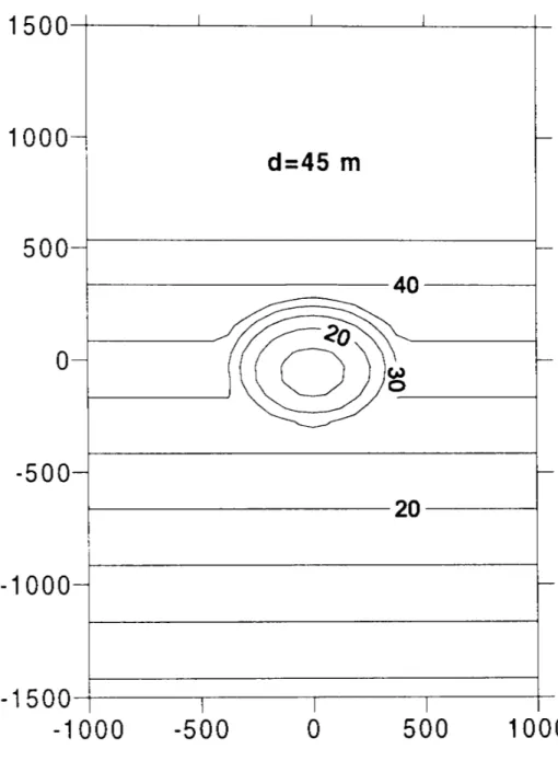
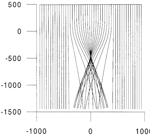
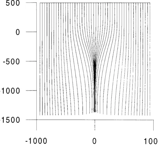
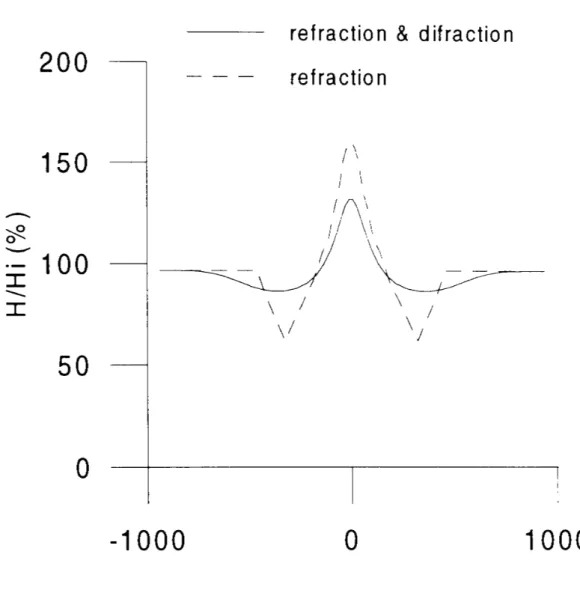
The model is tested first on the bottom topography shown in fig. 1, for an incoming wave train of period T=10 s, directed perpendicularly to the bed contours and in the sense of decreasing ordinates. Using a “classical” ray model, rays intersect each other behind the elliptic shoal, and a caustic turns up (fig. 2). When the refraction-diffraction model is used, the strong amplitude curvatures prior to the would-be caustic deflect the rays, preventing their intersection (fig. 3). The relative wave heights just in front of the caustic area (along the section y=-300 m) are shown (fig. 4) for both the pure refraction and the refraction-diffraction ray models. It can be seen that the consideration of diffraction leads to a more uniform distribution of energy, lowering the central peak and increasing the wave height in the adjacent low energy areas.
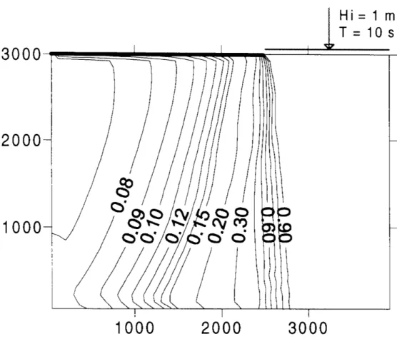
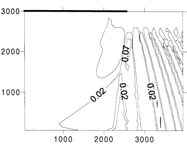
The model’s ability to deal with a strong variation of wave height, perpendicular to the direction of propagation, is demonstrated by considering the lee of a breakwater, depicted as a strong black line. In order to compare the results with Sommerfeld’s analytical solution, the depth is kept constant (d=20 m). Absolute wave heights are shown, for an incoming wave train with height H=1 m and period T=10 s (fig. 5). The maximum deviation with Sommerfeld’s solution, 0.08 m (8 %), is restricted to a small area, while the average values of the difference are significantly lower (fig. 6).
5 CONCLUSIONS
Wave propagation was calculated until the 70’s exclusively by means of the so-called ray methods, which consider the phenomenon of wave refraction. They fail in certain situations of interest primarily because of their neglect of a second phenomenon, diffraction.
The first mathematical model to deal simultaneously with both phenomena was introduced by Berkhoff4 in 1972. Thereafter many other propagation models have been presented, numerically based on finite differences, finite elements or boundary elements. They mostly omit the concepts of wave ray and wave front, obviously essential to ray methods.
In this paper a refraction-diffraction model in terms of rays and fronts is introduced. Its main feature is a new definition of the wave rays and, consequently, wave fronts, which considers both refraction and diffraction.
definition of rays as the characteristic lines of the eikonal equation of refraction-diffraction, together with the implementation of a ray-front coordinate system, reduce the energy equation to an ordinary differential equation, an important computational economy. Moreover the well-known limitations of the parabolic approximations in the lee of breakwaters or headlands are avoided. Finally, with the usual models – based on orthogonal or triangular grids – obtaining the wave fronts requires an interpolation with the values of the phase function at the grid nodes. In this model they are instead calculated directly, a more convenient procedure in many applications of Coastal Engineering. For instance, when it comes to studying the equilibrium plan shape of a beach.
REFERENCES
[1] E. Bouws and J. A. Battjes, “A Monte-Carlo approach to the computation of refraction of J. Geophys. Res., 87(C8), 5718-5722 (1982).
[2] A. Sommerfeld, “Mathematische Theorie der Diffraktion”, Mathematische Annalen, 47 (1896).
[3] W. G. Penney and A. T. Price, “The diffraction theory of sea waves and the shelter Phil. Trans. Roy. Soc. Lond., Ser. A, 244, 236-253 (1952). [4] J. C. W. Berkhoff, “Computation of combined refraction-diffraction”, Proc. 13th Int. Conf.
Coastal Engrg., 471-489 (1972).
[5] A. C. Radder, “On the parabolic equation method for water wave propagation”, J. Fluid Mech., 95(1), 159-176 (1979).
[6] C. Lozano and P. L.-F. Liu, “Refraction-diffraction model for linear surface water J. Fluid Mech., 101(4), 705-720 (1980).
[7] M. Isobe, “A parabolic refraction-diffraction equation in the ray-front coordinate system”, Proc. Int. Conf. On Coastal Engrg., 306-317 (1986).
[8] M. Isobe, “A parabolic equation model for transformation of irregular waves due to refraction, diffraction and breaking”, Coastal Engrg. In Japan, 30(1), 33-47 (1987). [9] N. Booij, “A note on the accuracy of the mild-slope equation”, Coastal Engrg., 7,