BEHAVIOR OF THE SECONDARY SOURCES AND EXAMINATION OF THE SOUND ENERGY FOR ACTIVE NOISE BARRIER

BEHAVIOR OF THE SECONDARY SOURCES AND EXAMINATION OF THE

SOUND ENERGY FOR ACTIVE NOISE BARRIER

PACS: 43.50.Ki

Hideo NAGAMATSU

Sekisui House Co. Ltd., 6-6-4 Souraku-gun Kizu Kyoto, 619-0224 JAPAN. Tel: +81(774) 73-1145

Fax: +81(774) 73–1181 E-mail: nagamatu@nifty.com;

Shiro ISE

Kyoto University, Yoshida-Honmachi, Sakyo-ku, Kyoto 606-8501 JAPAN. Tel: +81(75) 753-5725

Fax: +81(75) 753-5748

E-mail: ise@archi.kyoto-u.ac.jp;

Kiyohiro SHIKANO

Nara Institute of Science and Technology, 8916-5 Takayama-cho Ikoma Nara 630-0101 JAPAN, Tel: +81(743) 79-9886

Fax: +81(743) 72-5280

E-mail: shikano@is.aist-nara.ac.jp;

ABSTRACT

Without using the shielding thing, the active noise barrier (ANB) based on the boundary surface control can obstruct the sound by controlling the sound pressure and the acoustic impedance of the boundary surface. In this paper, we researched an appropriate arrangement of the secondary sources, and carried out the examination on the sound power output from the ANB. From the numerical analysis by boundary element method, it is desirable that the secondary sources are placed along the wave front made in the primary source.

INTRODUCTION

In recent years, the effectiveness of the ANB has been confirmed experimentally [1] [2]. However, in the same way as other applications of active noise control (ANC), the practical application of the ANB has its difficulties. In conventional studies of the ANB, the system has been focused on point control at an edge of a barrier or at a point around a barrier. Although this system is effective at the error sensor point, effectiveness in the area to be made quiet cannot be expected. This means that it is not possible to calculate the cost of the ANB that satisfies requirements of a client. In order to overcome these difficulties, it is necessary to construct a design method for the ANB that enables us to judge the scale of both the barrier and the ANC system [3] [4].

In this paper, we propose a design method for the ANB based on the boundary surface control (BSC) principle. This design method can generalize the specification of the ANB. However, the investigation on optimum arrangement of secondary sources and sensors is required. Further, the basic principle of this method is discussed by the numerical analysis based on the two-dimensional boundary element method (BEM).

ACTIVE NOISE BARRIER BASED ON THE BSC PRINCIPLE

velocity. The amplitudes of the secondary sources are set to minimize the acoustic energy at the sensor positions. Therefore, acoustic energy is reflected by the ANB at the position of sensor [5] [6].

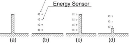
Fig.1. - Model of active noise barrier: (a) passive noise barrier; (b) active noise barrier; (c)(d) the combination of active noise barrier and passive noise barrier.

NUMERICAL CALCULATION

Determination of the Amplitudes of Secondary Sources When there are N noise sources of amplitude A’n at position s

’

n (n = 1LN) and Msecondary sources of amplitude A m′ at position s ′ m (m = 1LM), the sound pressure p(r) and particle velocity v(r) at position

r can be expressed as follows:

(1)

(2)

Where,

Hp(s|r) and Hv(s|r) are the transfer functions related to the pressure and the particle velocity between s and r. These transfer functions are calculated by BEM. Boundary S of the object control area is made discrete for K with the central coordinate of the boundary element as rk and the unit normal vector as nk (k = 1LK). Error judgment Je is defined as follows:

(3)

Je is an equivalent to the acoustic energy on boundary S. The amplitude of the secondary source that makes Je small, can be obtained by solving the equation for Am by applying Eq. (1), Eq. (2) and Eq. (3). Calculation Model

set to 2 m high and 10 m wide. The sound pressure level was calculated every 20 Hz in the range from 100 Hz to 1000 Hz.

Fig.2. - Two-dimensional model of numerical calculation.

Calculation Conditions

The sound pressure level was measured with 2, 4, 8, and 16 sensors attached at heights of 1, 2, and 3 m to the active and passive noise barriers (see (b) and (c) in Fig.1). The height of the passive barrier and the height of the sensor are the same. The condition name format is “X + number of sensors (secondary sources) + top sensor height + passive barrier height”. X16Y30 means that the number of sensors is 16, the top sensor height is 3 m, and the passive barrier height is 0 m (in other words, no barrier). The same number of sensors as secondary sources should be installed on the X-coordinate axis at equal height intervals. To make all the calculation intervals equal, the first sensor from the ground was installed with half the interval for other sensors.

RESULTS AND DISCUSSION

Optimum Arrangement of Secondary Sources

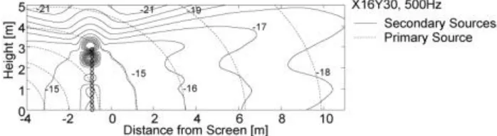
In order to examine the optimum arrangement of the secondary sources, the aspect of the sound pressure distribution only by the primary source and that only by the secondary sources was compared. With regard to the numeric calculation model shown in Fig. 2, a secondary source and an error sensor are installed at the same height as a pair. The sound pressure distribution by each source at 500 Hz of X16Y30 is shown in Fig.3.

Fig.3. - Sound pressure distribution of the secondary sources.

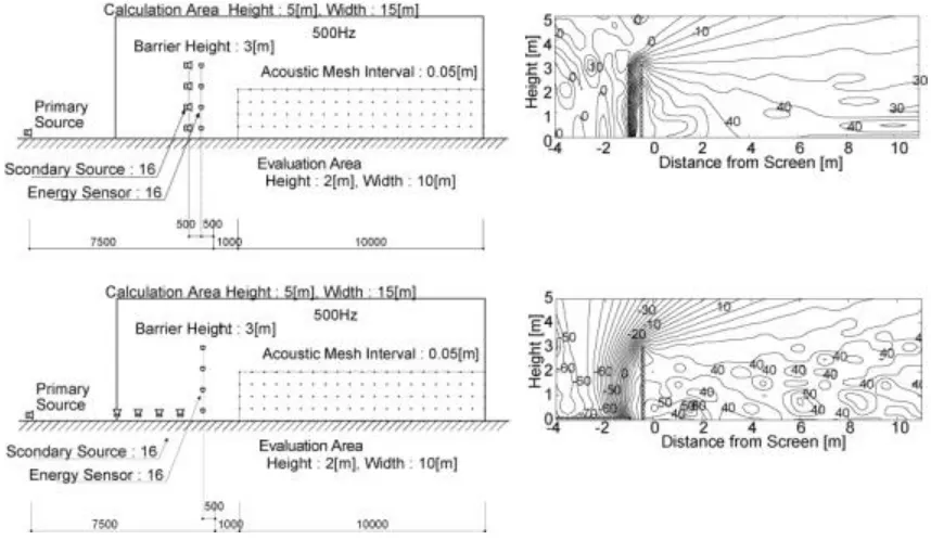
Fig.4. - Calculation Model and Sound pressure distribution.

Compared to X16Y30, this ground model is disadvantageous for creating the wave front of the primary source. Although a similar control effect is seen in the evaluation area, the sound pressure level on the side of the primary source is large and shows the sound pressure level rise of about 60 dB (Fig. 4). Therefore, the optimum arrangement of secondary sources is to place the sound sources along the wave front created by the primary source. Considering the sound source positions, the secondary sources should be arranged in parallel with the error sensors as shown in Fig. 2.

Insertion Loss

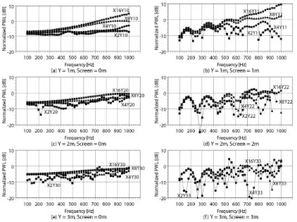
The insertion loss is the difference of the sound pressure level between with the barriers and without any barrier. It can be obtained as the energy average of difference in the evaluation area (105 calculation points in an area 10 m wide and 2 m high) of Fig. 2. To illustrate the control effects of the barriers, Fig. 5 shows the average power of the insertion loss without any barrier.

Fig.5. - Insertion loss against the barrier.

Power Level

This section discusses the power output level of the secondary sources compared to that of the primary source when the proposed ANB is used. A surrounding boundary ([O] in Fig. 6) was set one meter away from the primary source and the secondary sources, and the power level was calculated from the intensities on the boundaries.

Fig.6. - Intensity flow for: (a) only primary source; (b) only secondary sources.

Since the ground is set as the reflection surface, the lower half of the sound source was not considered. As Fig. 6 shows, the boundary of the secondary sources extends as the source height is raised. Fig. 7 shows the relative power level of the secondary sources. The power level of the secondary sources is smaller than that of the primary source. When the frequency becomes high, however, the power level goes up as the number of control points increases. The power level of the secondary sources is larger than that of the primary source at 700 Hz in the case of X16Y11, but not under other conditions. Fig. 5 (b), (d), and (f) show relative power levels when a passive barrier is installed. This mode appears because of the passive barrier.

Influence of Distance between Secondary Sources and Sensors

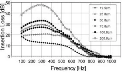
Fig. 8 shows the insertion losses where the secondary sources of X8Y30 are fixed, and the energy sensors are moved horizontally in parallel. The distances between secondary sources and sensors are 0.125, 0.25, 0.5, 0.75, 1, and 2 m. According to this figure, the value of the insertion loss increases, as the distance between energy sensors and secondary sources extends.

Fig.8. - Influence of distance between secondary sources and sensors.

CONCLUSION

If an ANB is used according to the design rules explained in this paper, its performance can be designed independently to that of a passive noise barrier. To increase the noise reduction effect, the sensor pitch should be reduced. For ANC control, the sensor pitch should be smaller than half the wavelength of the target noise. If the ANB produces a control effect, the noise level can be reduced by 10 dB or more compared to the case of a passive barrier alone. Even when the noise frequency is low and the sensor pitch is reduced to decrease the number of sensors, using a passive barrier together with an ANB ensures a sound insulation effect (by the conventional passive barrier) even at high frequencies where no control effect can be expected. Lastly, if the restrictions on installation area are eased, it is preferable to extend the interval between secondary sources and error sensors and to place the sound sources along the wave front created by the primary source.

BIBLIOGRAPHICAL REFERENCES

[1] S. Ise, H. Yano and H. Tachibana, “Basic study on active noise barrier”, J. Acoust. Soc. Jpn(E).,

vol.12, pp.299-306, 1991.

[2] A. Omoto and K. Fujiwara, “Basic study of active controlled noise barrier”, Proc. of

INTER-NOISE 91, pp.513-516, 1991.

[3] H. Nagamatsu, S. Ise and K. Shikano, “Numerical study of active noise barrier based on the

boundary surface control principle”, Proc. of Active 99, pp.585-594, 1999.

[4] H. Nagamatsu, S. Ise and K. Shikano, “Optimum arrangement of secondary sources and error

sensors for active noise barrier”, Proc. of INTER-NOISE2000, pp.1733-1738, 2000.

[5] S. Ise, “A principle of active control of sound based on the kirchhoff-helmholtz integral equation

and the inverse system”, Acustica, vol.85, pp.78-87, 1999.

[6] S. Ise, “Theory of acoustic impedance control for active noise control”, Proc. of INTER-NOISE 94,

pp.1339-1342, 1994.

[7] P. A. Nelson and S. J. Elliott, “Active control of sound”, Academic Press, London, pp.275-294,