An energy management strategy for plug-in hybrid electric vehicles

(1)

An Energy Management Strategy for Plug-in Hybrid Electric Vehicles

Tesi doctoral presentada per a l’obtenció del títol de Doctor per la Universitat Politècnica de Catalunya, dins el Programa de Doctorat en En-ginyeria Electrònica

Benjamin Bader

Director: Dr. José Luis Romeral Co-Director: Dr. Gerhard Lux

(2)

2

Abstract

This dissertation formulates a proposal for a real time implementable energy manage-ment strategy (EMS) for plug-in hybrid electric vehicles. The EMS is developed to minimize vehicle fuel consumption through the utilisation of stored electric energy and high-efficiency operation of powertrain components. This objective is achieved through the development of a predictive EMS, which, in addition to fuel efficiency, is optimized in terms of computational cost and drivability.

The requirement for an EMS in hybrid powertrain vehicles stems from the integration of two energy stores and converters in the powertrain; in the case of hybrid electric vehi-cles (HEVs) usually a combustion engine and one or more electric machines powered by a battery. During operation of the vehicle the EMS controls power distribution be-tween engine and electric traction motor. Power distribution is optimized according to the operating point dependent efficiencies of the components, energy level of the battery and trip foreknowledge. Drivability considerations, e.g. frequency of engine starts, can also be considered.

Powertrain hybridization is one of several measures which can increase vehicle fuel economy. Due to high oil prices and legislative requirements caused by the environ-mental impact of greenhouse emissions, fuel economy has gained importance in recent years. In addition to increased fuel economy, powertrain hybridization permits the sub-stitution of fuel for electrical energy by implementing an external recharging option for the battery. This vehicle class, incorporating a battery rechargeable via the electrical grid, is known as a plug-in HEV (PHEV). PHEV share characteristics of both HEVs and all-electric vehicles combining several advantages of both technologies.

(3)

3

These navigation systems and algorithms in combination with expected future advances and the deployment of technologies such as intelligent transport systems (ITS) and ve-hicle-to-vehicle communication (V2V), will make more exact traffic information avail-able to further improve prediction. Despite expected advances in prediction quality, inaccuracy of prediction data has to be considered and is therefore regarded in this work.

The EMS proposed in this dissertation combines different approaches which are exe-cuted step by step. A first approximation of the energy distribution during the trip is based on a mixed integer linear program (MILP), which gives the optimal energy state of the battery during the trip. This is especially important for trips with long uphill, downhill or urban phases, i.e. sections with a particularly high or lower power require-ment. The results from MILP are then used by a dynamic programming (DP) algorithm to calculate optimal torque and gear using a receding prediction horizon. Using a reced-ing prediction horizon, an important reduction of computational cost is achieved. Lastly, from the DP results a rule-based strategy is generated using a support vector machine (SVM). This last step is necessary to ensure the drivability of the vehicle also for inac-curate prediction data. The dissertation is organized as followed:

Firstly, the vehicle models employed in the dissertation and its validation are described. Secondly, a DP based algorithm is presented to compute the torque and gear during the trip. As DP is computational quite intensive, techniques are presented to lower the com-putational costs.

Thirdly, the DP algorithm is used in a model predictive control framework (MPC) with a receding prediction horizon. Necessary boundary condition of the battery state of charge (SOC) given by a SOC set point function for the entire trip are obtained using MILP.

(4)

4

List of Tables

Table I: Typical classification of HEV according to their level of hybridization. ... 19

Table II: Estimated vehicle component mass. ... 37

Table III: Values of the simulation parameters. ... 39

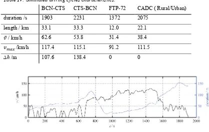
Table IV: Simulated driving cycles characteristics. ... 48

Table V: Deviation at specific operating points of the engine ... 52

Table VI: Average electrical energy consumption of the electric vehicle model for the NEDC ... 56

Table VII: Test vehicle characteristics measured on the chassis dynamometer ... 57

Table VIII: Comparison of fuel consumption for the NEDC ... 58

Table IX: Calculation times on an Intel i3 (1.8GHz) running Windows x64 ... 73

Table X: Simulation results for the BCN-CTS cycle. ... 74

Table XI: Simulation results for the FTP-72 cycle. ... 74

Table XII: Mechanical engine energy and electrical energy flow to and from the battery obtained by the MILP compared to the global optimum and relative difference d. ... 89

Table XIII: Average component efficiencies of electric motor (𝜂𝑒𝑚) and battery (𝜂_𝑏𝑎𝑡) of the global optimum. ... 89

Table XIV: Fuel consumption obtained by the MILP compared to the global optimum. ... 89

Table XV: Calculations times of the MILP (Intel i3 (1.8GHz) running Windows x64). ... 91

Table XVI: Relative deviation from the global optimum for different prediction horizon lengths (FTP-72 cycle). ... 94

Table XVII: Relative deviation from the global optimum for different prediction horizon lengths (BCN-CTS cycle). ... 95

Table XVIII: Simulation results for FTP-72 cycle for different prediction horizon lengths. ... 96

Table XIX: Simulation results for BCN-CTS cycle for different prediction horizon lengths. ... 96

Table XX: Simulation results for the cycles FTP-72 and BCN-CTS. ... 115

Table XXI: Simulation results of CS operation (FTP-72 cycle) with 𝑁_𝑐 = 60 using the estimation 𝑆𝑂𝐶 from Eq. (5.24). ... 116

Table XXII: Calculation time of the rule adaptation by SVM. ... 117

Table XXIII: Simulation results for CS operation (FTP-72 cycle). ... 118

Table XXIV: Simulation results for CD operation (BCN-CTS cycle). ... 118

Table XXV: Relative difference to the global optimum for different prediction horizon lengths - simulation results for the cycles FTP-72 and BCN-CTS. ... 118

(7)

7

Table XXVII: Global optimum and EMS battery energy flow with 𝑁_𝑝 = 200. ... 120 Table XXVIII: Simulation results and deviation from the global optimum for the

FTP-72 cycle using different prediction horizon lengths. ... 121 Table XXIX: Simulation results for CD mode for the BCN-CTS cycle. ... 121 Table XXX: Relative difference to the global optimum of the strategy EMS with

𝑁𝑝= 200 of the cycles CADC and CTS-BCN. ... 124 Table XXXI: Simulation results and deviation from the global optimum for

rule-based strategy in CS mode (FTP-72 cycle) and 𝑁𝑝 = 200. ... 126

Table XXXII: Simulation results and deviation from the global optimum for CD

(8)

8

List of Figures

Fig. 1.1. Transportation sector greenhouse gas emissions (energy transformation

emissions not included) in the EU in 2009. ... 15

Fig. 1.2. Road transportation contribution to the transportation sector greenhouse gas emissions in the EU in 2009. ... 15

Fig. 1.3. Crude oil price development from 1981 to 2012 in US $ (Index 1991=100). ... 16

Fig. 1.4. Development of average CO2 emissions of new passenger cars in the EU. The cars are classified into petrol, diesel and alternative fuel vehicles (AFV) including (P)HEVs. ... 17

Fig. 1.5. Indirect CO2 emissions of battery electric vehicles by region. ... 18

Fig. 1.6. Ratio of typical trip distances of passenger cars in Europe, the USA and Japan... 20

Fig. 1.7. Cumulative ratio of typical trip distances of passenger cars in Europe, the USA and Japan. ... 20

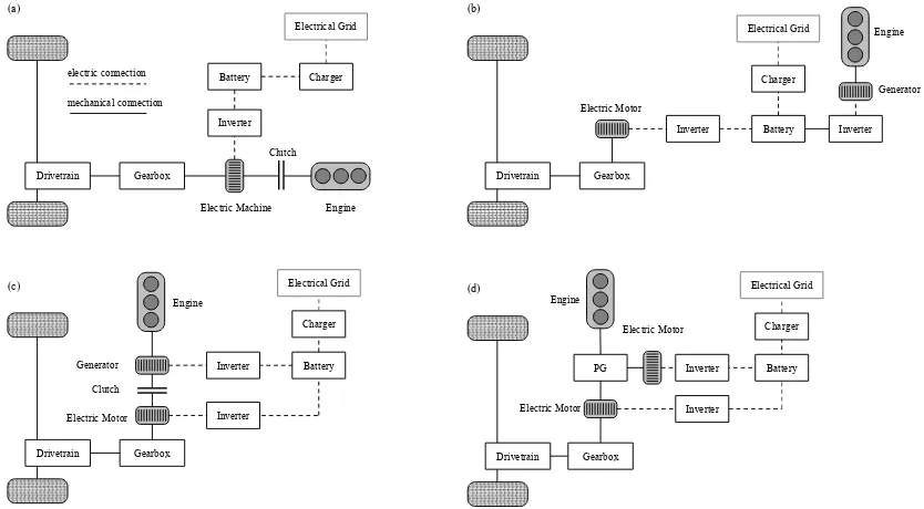
Fig. 1.8. Hybrid powertrain configurations: parallel (a), serial (b), serial/parallel (c) and power-split with a planetary transmission (d). ... 22

Fig. 1.9. Operation modes of a parallel PHEV. ... 23

Fig. 1.10. Load point shifting. Engine operating points in the specific fuel consumption map. ... 23

Fig. 1.11. Communication between EMS and powertrain components. ... 25

Fig. 1.12. Energy management problem for PHEV. ... 25

Fig. 1.13. SOC during the BCN-CTS cycle using an AER-focused strategy. ... 26

Fig. 1.14. SOC during the BCN-CTS cycle using a blended strategy. ... 26

Fig. 1.15. Operation modes during the driving cycle BCN-CTS using an AER-focused strategy... 26

Fig. 1.16. Operation modes during the driving cycle BCN-CTS using a blended strategy. ... 27

Fig. 1.17. Engine operating points using an AER-focused strategy during BCN-CTS. ... 27

Fig. 1.18. Engine operating points using a blended strategy during BCN-CTS. ... 27

Fig. 1.19. Information used by load forecasting algorithms for trip prediction. ... 29

Fig. 1.20. Use of stored electrical energy during a trip. ... 32

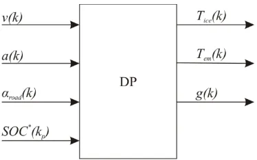
Fig. 1.21. The EMS uses trip prediction data and the current SOC, in an MPC framework, to calculate the optimal torque and gear of the trip within the prediction horizon. ... 33

Fig. 2.1. Principle of the vehicle forward model. ... 35

Fig. 2.2. Principle of the vehicle backward model. Vehicle speed corresponds exactly to the driving cycle speed. ... 35

(9)

9

Fig. 2.4. Measured maximal torque of electric motor, combustion engine and its

sum 𝑇𝛴,𝑚𝑎𝑥 at the transmission input. ... 37

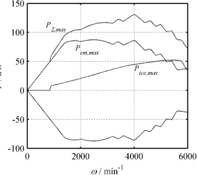
Fig. 2.5. Measured maximal power of electric motor, combustion engine and the sum 𝑃𝛴,𝑚𝑎𝑥 at the transmission input. ... 37

Fig. 2.6. Measured specific fuel consumption map and optimal consumption line 𝑇𝑖𝑐𝑒,𝑠𝑝𝑐,𝑚𝑖𝑛 of the combustion engine. ... 38

Fig. 2.7. Measured electric motor efficiency map. ... 38

Fig. 2.8. Battery clamp power and chemical power for a SOC of 0.3 and 0.9. ... 43

Fig. 2.9. Battery efficiency as a function of its chemical power. ... 43

Fig. 2.10. Linear vehicle model variables. ... 44

Fig. 2.11. Willans lines of the engine at different engine speeds. ... 45

Fig. 2.12. Approximation of the electric machine efficiency in motoring mode. ... 46

Fig. 2.13. Approximation of the electric machine efficiency in generating mode ... 46

Fig. 2.14. Road slope 𝛥ℎ and angle of inclination 𝛼_{𝑟𝑜𝑎𝑑}. ... 46

Fig. 2.15. Speed and elevation profile of the driving cycle BCN-CTS. ... 48

Fig. 2.16. Speed and elevation profile of the driving cycle CTS-BCN. ... 48

Fig. 2.17. Speed profile of the driving FTP-72 cycle. ... 48

Fig. 2.18. Speed profile of combined rural and urban part of the CADC. ... 49

Fig. 2.19. Vehicle model communication with dynamometer test bench. ... 50

Fig. 2.20. Control structure of the test bench. ... 50

Fig. 2.21. Conventional vehicle model structure for HIL simulation. ... 51

Fig. 2.22. NEDC speed profile. ... 51

Fig. 2.23. Dynamometer test bench configuration for the conventional powertrain. ... 53

Fig. 2.24. Comparison between HIL measurements of the conventional powertrain and offline simulation results during the urban section of the NEDC. ... 53

Fig. 2.25. Comparison between HIL measurements of the conventional powertrain and offline simulation results during the extra urban section of the NEDC. ... 53

Fig. 2.26. Test bench configuration of the electric powertrain system with the engine decoupled from the powertrain... 54

Fig. 2.27. Comparison of output current and voltage of the battery simulator and offline model during the NEDC. ... 54

Fig. 2.28. Measured and simulated battery output power 𝑃_𝑖𝑛𝑣_,_𝐷𝐶, electric motor torque 𝑇𝑒𝑚 and electric motor speed 𝜔𝑒𝑚. ... 55

Fig. 2.29. SOC of HIL measurement and offline simulation during NEDC. ... 56

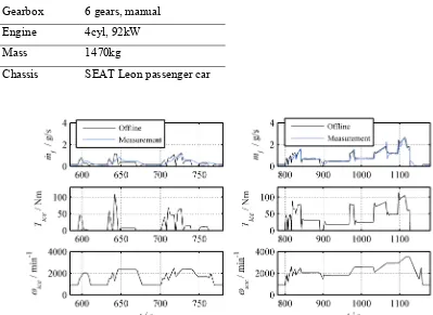
Fig. 2.30. Comparison of simulated and measured fuel mass flow during the fourth urban section and the extra urban section of the NEDC. ... 57

Fig. 2.31. Comparison of measured fuel mass flow on chassis dynamometer during first (engine cold) and fourth urban part (engine warm) of the NEDC cycle. .... 58

Fig. 3.1. Optimization of torque and gear for a trip (DP input/output). ... 60

Fig. 3.2. Dynamic programming shortest path search for CD operation). ... 62

Fig. 3.3. Combination of the electric motor loss table and its inverse. ... 64

(10)

10

Fig. 3.5. Validation of the inverse 2D lookup table by connecting both tables in

series and comparing the input and output value. ... 65

Fig. 3.6. 3-dimensional lookup table array 𝑭_𝑚_𝑓 for the accelerated DP algorithm (A-DP). ... 68

Fig. 3.7. Maximal influence of the rounding error 𝑒𝑃 on the torque 𝑇𝑤ℎ. ... 70

Fig. 3.8. Effect of the rounding error 𝑒𝑣 on the torque 𝑇𝑤ℎ. ... 70

Fig. 3.9. Difference between torque obtained by S-DP and A-DP for the FTP-72 cycle at seconds 35-50 and 70-90. ... 72

Fig. 3.10. Difference between torque obtained by S-DP and A-DP for the BCN-CTS cycle during seconds 200-250 and 1450-1500. ... 73

Fig. 3.11. Electric motor torque 𝑇𝑒𝑚 obtained by A-DP (above), S-DP (middle) and the difference 𝛥𝑇_𝑒𝑚 (bottom) during the BCN-CTS cycle. ... 75

Fig. 3.12. Engine torque 𝑇𝑖𝑐𝑒obtained by A-DP, S-DP and the difference 𝛥𝑇𝑖𝑐𝑒 for the BCN-CTS cycle. ... 75

Fig. 3.13. SOC during driving cycle FTP-72 obtained by S-DP and A- DP. ... 75

Fig. 3.14. SOC during driving cycle BCN-CTS obtained by S-DP and A-DP. ... 76

Fig. 4.1. Exemplary set point function 𝑆𝑂𝐶∗₍_𝑘₎_{for optimization using a receding} prediction horizon. ... 77

Fig. 4.2. Example of a set of feasible solutions with level sets of the objective function (3x1+2x2). ... 79

Fig. 4.3. Interior path of path following method. ... 80

Fig. 4.4. The SOC set point functions 𝑆𝑂𝐶𝑙𝑖𝑛∗ (𝑘) and 𝑆𝑂𝐶𝑀𝐼𝐿𝑃∗ (𝑘) for the BCN-CTS cycle compared to the global optimal SOC. ... 84

Fig. 4.5. SOC set point function for the CADC compared to the global optimum. ... 85

Fig. 4.6. SOC set point function for CTS-BCN cycle compared to the global optimum. ... 85

Fig. 4.7. SOC set point function for FTP-72 cycle compared to the global optimum. ... 85

Fig. 4.8. Power distribution for the cycle CTS- BCN obtained by the MILP. ... 86

Fig. 4.9. Power distribution for the cycle CTS-BCN obtained by the DP. ... 86

Fig. 4.10. Specific consumption of the engine model used for calculation of the global optimum. ... 88

Fig. 4.11. Specific consumption of the convex engine model. ... 88

Fig. 4.12. Engine model approximation at low engine power. ... 89

Fig. 4.13. Power distribution obtained by the MILP for the CADC. ... 90

Fig. 4.14. Power distribution obtained by the MILP for the FTP-72 cycle. ... 90

Fig. 4.15. Optimal power distribution during the BCN-CTS cycle obtained by the MILP. ... 90

Fig. 4.16. Global optimal power distribution during the BCN-CTS cycle. ... 90

Fig. 4.17. Idealized calculation of the predictive optimization using an MPC framework. ... 92

(11)

11

Fig. 4.19. Calculation time of the DP during the BCN-CTS cycle as a function of

the prediction horizon length. ... 93

Fig. 4.20. SOC during FTP-72 cycle employing CS mode for different prediction horizon lengths and the global optimum. ... 94

Fig. 4.21. SOC during BCN-CTS cycle employing CD mode for different prediction horizon lengths and the global optimum... 94

Fig. 4.22. Results for FTP-72 cycle as a function of the prediction horizon length. ... 95

Fig. 4.23. Results for the BCN-CTS cycle as function of the prediction horizon length. ... 95

Fig. 5.1. Typical rule-based EMS for parallel HEV in terms of motor torque and vehicle speed. ... 99

Fig. 5.2. Operation modes as a function of vehicle speed 𝑣 and power request 𝑃𝑟𝑒𝑞. 100 Fig. 5.3. Block diagram of the complete EMS. ... 101

Fig. 5.4. Flowchart of the rule-based strategy. ... 102

Fig. 5.5. 𝑇𝑖𝑐𝑒 with minimal ratio min(𝑚𝑓/𝑃𝑟𝑒𝑞) as function of 𝜔𝑒𝑚 and 𝑃𝑟𝑒𝑞. ... 103

Fig. 5.6. 𝑇𝑒𝑚 with minimal ratio min(𝑚𝑓/𝑃𝑟𝑒𝑞) as function of 𝜔𝑒𝑚 and 𝑃𝑟𝑒𝑞. ... 103

Fig. 5.7. Torque error caused by using lookup tables as a function of 𝜔_𝑒𝑚. ... 104

Fig. 5.8. Torque error caused by using lookup tables as a function of 𝑃𝑟𝑒𝑞. ... 104

Fig. 5.9. Optimal gear 𝑔ℎ𝑦𝑏𝑟𝑖𝑑 in terms of fuel mass flow in ICE mode with 𝑃𝑏𝑎𝑡 = 0𝑘𝑊. ... 106

Fig. 5.10. Optimal gear 𝑔ℎ𝑦𝑏𝑟𝑖𝑑 in terms of fuel mass flow in boost mode (𝑃𝑏𝑎𝑡 = 10𝑘𝑊). ... 106

Fig. 5.11. Optimal gear 𝑔_{ℎ𝑦𝑏𝑟𝑖𝑑}in terms of fuel mass flow in charge mode (𝑃_𝑏𝑎𝑡 = −10𝑘𝑊). ... 106

Fig. 5.12. Gear shifting schedule 𝑔_𝑒𝑚 in electric mode. ... 107

Fig. 5.13. Gear shifting schedule 𝑔𝑖𝑐𝑒 in hybrid mode. ... 107

Fig. 5.14. Optimal hyperplane separator of patterns from two different classes [97]. . 109

Fig. 5.15. Separator 𝑃ℎ𝑦𝑏𝑟𝑖𝑑 between electric mode and hybrid mode at different times during the BCN-CTS cycle calculated using SVM. ... 110

Fig. 5.16. Separator 𝑃ℎ𝑦𝑏𝑟𝑖𝑑 between electric mode and hybrid mode at different times during the FTP-72 cycle calculated using SVM. ... 110

Fig. 5.17. Rule-based strategy 600 seconds into the BCN-CTS cycle obtained from (𝒖_𝑖𝑜𝑝𝑡) for the marked trip section and resulting operating points ... 111

Fig. 5.18. Rule-based strategy 1800 seconds into the BCN-CTS cycle obtained from (𝒖_𝑖𝑜𝑝𝑡) for the marked trip section and resulting operating points. ... 111

Fig. 5.19. Operation modes during the BCN-CTS cycle selected by the rule-based EMS. ... 112

Fig. 5.20. Engine torque 𝑇_𝑖𝑐𝑒during the BCN-CTS cycle of the global optimum and the rule-based EMS. ... 112

Fig. 5.21. Operation modes during the FTP-72 cycle selected by the rule-based EMS. ... 113

(12)

12

Fig. 5.23. Engine operating points during BCN-CTS using the rule-based EMS. ... 113

Fig. 5.24. Global optimum engine operating points during FTP-72. ... 113

Fig. 5.25. Engine operating points during FTP-72 using the rule-based EMS. ... 113

Fig. 5.26. Hybrid mode during BCN-CTS. ... 114

Fig. 5.27. Engine torque 𝑇𝑖𝑐𝑒during FTP-72 cycle of rule-based EMS and global optimum. ... 114

Fig. 5.28. Gear during the BCN-CTS cycle of rule-based EMS and global optimum. 115 Fig. 5.29. SOC during the FTP-72 cycle of the rule-based EMS and the global optimum. ... 115

Fig. 5.30. SOC during the BCN-CTS cycle of the rule-based EMS and the global optimum. ... 115

Fig. 5.31. SOC during FTP-72 cycle with 𝑁_𝑐 = 60 using the estimation 𝑆𝑂𝐶 from Eq. (5.24)... 117

Fig. 5.32. Component losses for the different cycles compared to the global optimum. ... 120

Fig. 5.33. Global optimum engine run time during the BCN-CTS cycle. ... 121

Fig. 5.34. Engine run time during the BCN-CTS cycle (EMS with 𝑁𝑝 = 200). ... 121

Fig. 5.35. Global optimum engine run time during the FTP-72 cycle. ... 121

Fig. 5.36. Engine run time during the FTP-72 cycle (EMS with 𝑁𝑝 = 200). ... 121

Fig. 5.37. Engine operating points during the CADC (global optimum). ... 123

Fig. 5.38. Engine operating points during the CADC (EMS with 𝑁𝑝 = 200). ... 123

Fig. 5.39. SOC during the CTS-BCN cycle with 𝑁_𝑝 = 200. ... 123

Fig. 5.40. Operation modes during CTS-BCN cycle (global optimum). ... 123

Fig. 5.41. Operation modes during CTS-BCN cycle (EMS, 𝑁𝑝 = 200). ... 124

Fig. 5.42. Distorted prediction data (DPD1 and DPD2) for BCN-CTS cycle. ... 125

Fig. 5.43. Distorted prediction data (DPD1 and DPD2) for FTP-72 cycle. ... 125

Fig. 5.44. Hybrid mode during BCN-CTS cycle (DPD1). ... 126

Fig. 5.45. Engine operating points during the FTP-72 cycle (𝑁_𝑝 = 200, DPD1). ... 127

Fig. 5.46. Engine operating points during the FTP-72 cycle (𝑁𝑝 = 200, DPD2). ... 127

Fig. 5.47. Engine operating points during the BCN-CTS cycle (𝑁𝑝 = 200, DPD1). .. 127

(13)

13

List of Symbols

𝛼𝑎𝑐𝑐 accelerator pedal position

𝛼𝑏𝑟𝑎𝑘𝑒 brake pedal position

𝛼𝑟𝑜𝑎𝑑 angle of road inclination

𝑎 longitudinal vehicle acceleration 𝐴𝑓 vehicle frontal area

𝑐𝑤 vehicle drag coefficient

𝐸𝑏𝑎𝑡,𝑚𝑖𝑛 minimum battery energy level

𝐸𝑏𝑎𝑡,𝑚𝑎𝑥 maximum battery energy level

𝐸𝑏𝑎𝑡,𝑛𝑜𝑚 nominal battery energy capacity

𝐸𝑏𝑎𝑡 stored chemical energy in battery

𝑓𝐵𝑊 nonlinear vehicle backward model

𝑓𝑀𝐼𝐿𝑃 linear vehicle model

𝐹𝑤ℎ traction wheel force

𝑔 gear

𝑔𝑟 gear ratio (including final ratio)

Δℎ road slope

𝐽𝑤ℎ wheel inertia (sum of all four wheels)

𝑚 vehicle mass

𝑚̇𝑓 engine fuel mass flow

𝑃𝑏𝑎𝑡 chemical battery power

𝑃𝑐𝑦𝑐𝑙𝑒 wheel power requirement for driving cycle

𝑃𝑒𝑚,𝑚𝑎𝑥 maximum mechanical power of the electric motor as a fuction of 𝜔𝑒𝑚

𝑃𝑒𝑚 mechanical power of the electric motor

𝑃𝑖𝑐𝑒,𝑚𝑎𝑥 maximum mechanical power of the engine as a fuction of 𝜔𝑖𝑐𝑒

(14)

14

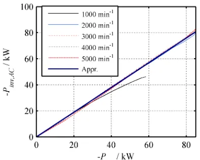
𝑃𝑖𝑛𝑣,𝐴𝐶 electrical power at AC (motor) side of the inverter

𝑃𝑖𝑛𝑣,𝐷𝐶 electrical power at DC (battery) side of the inverter

𝑃𝑤ℎ wheel power

𝑅𝑏𝑎𝑡 battery internal resistance

𝑟𝑤ℎ dynamic wheel radius

𝑇𝑒𝑚,𝑚𝑎𝑥 maximum electric motor torque as a function of 𝜔𝑒𝑚

𝑇𝑒𝑚 electric motor torque

𝑇𝑖𝑐𝑒 engine torque

𝑇𝑖𝑐𝑒,𝑚𝑎𝑥 maximum engine torque as a function of 𝜔𝑖𝑐𝑒

𝑇𝑟𝑒𝑞 torque requested by driver

𝜂𝑒𝑚 electric motor efficiency

𝜂𝑖𝑛𝑣 inverter efficiency

𝜂𝑡𝑟𝑎𝑛𝑠 transmission and drivetrain efficiency

𝑁𝑐 control horizon length

𝑁𝑝 prediction horizon length

𝜇𝑟 vehicle rolling resistance

𝒖 control vector

Δ𝑡 sample time

𝑆𝑂𝐶0 battery state of charge at trip start

𝑆𝑂𝐶𝑒𝑛𝑑 battery state of charge at end of trip

𝑆𝑂𝐶 battery state of charge

𝑆𝑂𝐶� estimated battery state of charge

𝑣 vehicle speed

𝑣𝑐𝑦𝑐𝑙𝑒 driving cycle vehicle speed

𝑉0 nominal battery voltage

𝜔𝑒𝑚 electric motor shaft speed

𝜔𝑖𝑐𝑒 combustion engine shaft speed

(15)

15

1 Introduction

1.1 Background and Motivation

In recent years, the issue of fuel economy in the development of transportation vehicles has gained increasing importance. This is mainly due to:

• the assumed impact of carbon dioxide (CO2) on the climate • legislative requirements

• the increasing price of oil and uncertainty over future price changes.

In 2009, transportation sector emissions amounted to 25% of the European Union (EU)’s total greenhouse gas emissions1_{, and 29.9% of its CO}

2 emissions. The contribu-tion of road-only transport (i.e. cars, trucks and buses) to the transportacontribu-tion sector’s total greenhouse gas emissions is 71.7%, which still corresponds to more than 14% of the EU’s total emissions [1]. Taking into account the emissions caused by the complete energy transformation process (mines, plants, refineries, pipelines, etc.) to calculate end-user emissions, the figure of transportation sector greenhouse gas emissions rises to 29% [2]. Consequently, in 2009 legal requirements were made for car manufacturers to reduce the average CO2 emissions of their fleet to 130g/km by 2015 and to 95g/km by 2020 [3].

Fig. 1.1. Transportation sector greenhouse gas emissions (energy transformation emis-sions not included) in the EU in 2009 [1].

Fig. 1.2. Road transportation contribution to the transportation sector greenhouse gas emissions in the EU in 2009 (energy transfor-mation emissions not included) [1].

1_CO

2 equivalent emissions

Other (75%)

Transportation (25%)

Railway (0,6%)

Road Transportation (71.7%)

Total Navigation

(16)

16

In addition to environmental issues, the development of fuel efficient vehicles is moti-vated by economic factors, principally rising fuel prices over the last ten years. This price increase is mainly due to rising fuel duty and oil prices on the world markets (Fig. 1.3). Although new oil extraction techniques have been developed (tar sands in Canada and deep sea extraction off the coasts of Brazil and Nicaragua), the higher costs of these processes and the increased demand from developing countries have driven oil prices to new heights. Future oil price development is difficult to predict2_{, but with rising}

extrac-tion and producextrac-tion costs, a return to the low oil prices of the past seems improbable.

Fig. 1.3. Crude oil price development from 1981 to 2012 in US $ (Index 1991=100) [4].

Reduced fuel use brings political and economic benefits for oil importing countries - lesser dependence on politically unstable oil-producing regions, reduced impact of po-tential future oil shortages, and a positive effect on the domestic economy through re-duced imports. Other advantages are rere-duced environmental damage, a reduction in global warming and climate change and its associated extreme weather phenomena. Summarising the above, increased fuel economy in automobiles is highly desirable. Driven by increasing customer demand, manufacturers have already taken measures with vehicles using a conventional powertrain, i.e. a powertrain driven only by a com-bustion engine. Among those measures are the reduction of the vehicle’s air drag coef-ficient, the use of lightweight materials, engine downsizing and temporary cylinder de-activation (“dynamic downsizing”). Major advances have been made in this area in re-cent years, resulting in a steady reduction in fuel consumption (Fig. 1.4). Another ap-proach for fuel saving is the powertrain hybridization. Hybridization is the integration of an additional energy store and energy converter within a conventional powertrain. Usually, this is an electric motor with electrical energy store, which is normally an elec-trochemical battery or supercapacitor. Vehicles using this type of hybrid powertrain are

2_{In 2004 the International Energy Agency (IEA) predicted a crude oil price of 22$ / barrel for 2012. The}

actual price in 2012 was more than 100$ / barrel. 0

100 200 300 400 500 600 700

1991 1992 1993 1994 1995 1996 1997 1998 1999 2000 2001 2002 2003 2004 2005 2006 2007 2008 2009 2010 2011 2012

Inde

x

(1991

=

100)

(17)

17

called hybrid electric vehicles (HEV). The additional electrical energy store and electric motor permit that some of the vehicle’s kinetic energy can be regenerated while braking by operating the electric motor in generating mode. In addition, traction power demand can be decoupled in terms of time from the mechanical power output of the engine within certain limits. Therefore, the combustion engine can operate in higher efficiency regions. This is especially advantageous in urban traffic, which is characterised by fre-quent braking, long idle times and low engine load - while on motorways with their higher load profile the engine can operate without additional measures in high effi-ciency regions. Powertrain hybridization can be classified into different levels, accord-ing to the maximum power of the electric motor and the electrical energy store capacity. Vehicles with high levels of hybridization incorporate electric powertrain components which are similar in nominal electric motor power and battery capacity to all-electric vehicles, as e.g. battery electric vehicles (BEVs). HEVs with an energy storage system capacity comparable to BEVs, i.e. with an energy capacity of at least 4kWh, can re-charge the battery not only by means of the engine but also by connection to the electri-cal grid (plug-in HEVs). These plug-in HEVs (PHEVs) have a more limited electric driving range than BEVs, but with the option of refilling with gasoline and thereby of-fering practically unlimited driving range.

Fig. 1.4. Development of average CO2 emissions of new passenger cars in the EU. The cars are

classified into petrol, diesel and alternative fuel vehicles (AFV) including (P)HEVs [5].

By substituting fuel for electrical energy in vehicles, CO2 emissions can be reduced sig-nificantly. In contrast to using fuel, when using electrical energy to propel the vehicle emissions are not generated directly by the vehicle, but at the power plants where the electricity is generated. Therefore CO2 emissions depend on the methods of power gen-eration and fuel type used at the power plant. In regions where large proportions of total energy output are generated by renewable sources (hydro-plants, wind/solar plants, etc)

0 50 100 150 200 250

2000 2001 2002 2003 2004 2005 2006 2007 2008 2009 2010 2011 2012

gCO

2

/ k

m

Year Petrol

(18)

18

such as Sweden or Switzerland, the resulting CO2 emissions are low. However, in re-gions where coal is the main source for power generation, emissions can be higher than those generated by conventional powertrain configurations without an electric motor (Fig. 1.5). Therefore, to be effective in reducing emissions, widespread use of PHEVs and BEVs must go hand-in-hand with clean electricity generation. The impact of wide-spread use of BEVs or PHEVs on electrical power generation would be minor, as the generated electrical grid load would be relatively small. In Germany, the additional electrical energy requirement of 10 million BEVs amounts to only 3% of current total electrical power production [6].

Fig. 1.5. Indirect CO2 emissions of battery electric vehicles by region. Calculation based on a

BEV with an electrical energy consumption of 18kWh/100km and a charging efficiency of 0.95 using data from [7].

1.2 Introduction to Hybrid Powertrain Concepts

Hybrid vehicles can have non-electric energy storage system such as flywheels [8], or, as in hydraulic hybrid vehicles, compressed gas [9] In the following work, only HEV concepts with electrical energy store are discussed, as they not only increase powertrain efficiency, but PHEVs can also substitute fuel for electrical energy as the traction en-ergy source. HEVs have in addition to the fuel based enen-ergy store (natural gas, gasoline, diesel, hydrogen) an electrical energy store which is normally an electrochemical bat-tery or a supercapacitor [10]. This electrical energy store supports bidirectional power transfer, i.e. it can both store and deliver energy. For PHEVs and most HEVs, this en-ergy store is a battery and the fuel based enen-ergy store a petrol tank. In the following work, discussion is limited to (P)HEVs of this type.

There are a variety of different HEV concepts, which can be classified in terms of their level of hybridization or their powertrain configuration. HEV powertrain configurations differ in the number of electric machines they incorporate and in the manner in which

0 20 40 60 80 100 120 140 160 180 EU

Greece Switzerland

(19)

19

they are physically connected to the combustion engine and wheels. The level of hy-bridization is defined by the power rating of the electric machine and battery capacity. Increasing levels of hybridization brings on the one hand benefits in the area of fuel economy, but on the other hand, higher fabrication costs. Conventional vehicles have the lowest level of hybridization (powertrain without electric components), and electric vehicles like BEVs with only electric powertrain components have the highest levels of hybridization. Between them, there are (in order of level of hybridization): micro HEVs, mild HEV, and full HEVs. There are no standardised definitions for the levels, and their definitions in literature are inconsistent. A typical classification is indicated in Table I. Micro HEVs support mainly an engine start/stop function to reduce engine idle times and limited kinetic energy regeneration. Mild HEVs have a higher level of hybridization and support energy regeneration at higher loads, and load point shifting of the engine. Full HEVs with their stronger electric motor can, in addition, drive electrically. Vehi-cles with higher battery capacities have a battery charger onboard, which permits bat-tery charging by connection to the electrical grid. HEVs with this charging capability are called plug-in HEVs (PHEVs).

Table I: Typical classification of HEV according to their level of hybridization.

Micro HEV Mild HEV Full HEV PHEV BEV

𝑃𝑒𝑚.𝑚𝑎𝑥 < 6 kW <25 kW 25-125 kW 50-125 kW 50-125 kW

𝐸𝑏𝑎𝑡,𝑛𝑜𝑚 <0.1kWh <0.1kWh <2kWh > 4kWh >12kWh

𝑉0 <24V <60V <600V <600V <600V

(20)

20 Fig. 1.6. Ratio of typical trip distances of pas-senger cars in Europe, the USA and Japan [11].

Fig. 1.7. Cumulative ratio of typical trip dis-tances of passenger cars in Europe, the USA and Japan [11].

1.2.1 Hybrid Powertrain Configurations

In addition to the level of hybridization, HEV can also be classified in terms of the me-chanical connections between engine, electric machines and wheels. There are four dif-ferent configuration types: the series, parallel, series/parallel and power split concept. These configurations will now be briefly discussed.

All concepts include a battery, inverter and at least one electric machine. The exemplary vehicle in this work has a parallel powertrain, in which both the electric motor and the engine are mechanically connected to the wheels, so that the sum of electric motor and engine power propels the vehicle. The mechanical connection between engine and elec-tric motor can be made using torque addition (the most common type); speed addition, incorporating a planetary gear; or traction force addition by connecting the electric mo-tor and engine to the different driving axles [12]. In the exemplary vehicle, mo-torque addi-tion is achieved by mounting engine and electric motor on a common shaft (Fig. 1.8). An advantage of the parallel configuration is that the electric powertrain components can be relatively easily integrated into conventional powertrains. Due to the direct me-chanical connection of engine and drivetrain, engine power can be used for driving without the transformation losses which occur in the series concept. In parallel full HEV, the engine can usually be separated by a clutch from the rest of the powertrain to prevent friction losses when the vehicle is propelled electrically.

When the engine cannot be separated by a clutch, the configuration is referred to as a torque assist parallel hybrid. In [13] it is demonstrated that a torque assist hybrid has lower fuel economy compared with a full parallel hybrid with an identical level of

hy-0 5 10 15 20 25 30 35 ra tio / %

trip distance / km US EU JP 0 10 20 30 40 50 60 70 80 90 100

0 50 100

Cu m ul at iv e ra tio / %

(21)

21

bridization. Therefore, this configuration is not common for powertrains with a high level of hybridization.

In contrast to the parallel configuration, in the series configuration only the electric trac-tion motor has a mechanical connectrac-tion with the wheels. The engine is coupled to a generator which delivers electrical energy to supply the electric traction motor. A bat-tery is used as an energy buffer. A significant drawback of this configuration is that the engine power always suffers transformational losses via the conversion chain (engine-generator-inverter-electric motor). On the other hand, due to the energy buffer, the en-gine can operate in high efficiency regions and with slow operating point change, result-ing in lower emissions of unburned hydrocarbons (HC) and carbon monoxide (CO). Wheel hub motors can also be used in this concept.

As only the electric motor is used to power the vehicle, drivability is better than with parallel full HEVs due to less engine starts and gear shifts. Having a mechanical con-nection between electric motor and wheels only, also results in greater freedom in the placement of components in the vehicle. Series HEV with an energy store capacity comparable to PHEV or BEV and which is chargeable via the electrical grid is referred to as a range extender configuration, as it is considered an electric vehicle with onboard charging unit.

Adding a mechanical connection between engine and electric traction motor to the se-ries configuration, results in a sese-ries-parallel configuration. This configuration com-bines advantages of both series and parallel concepts, such as an increased number of available operation modes (for operation modes see Section 1.2.2), but at the cost of increased fabrication cost. In order to reduce costs and complexity, a two-speed gearbox between drivetrain and powertrain can be used, limiting engine use at lower vehicle speeds to the series operation mode. The power-split configuration is another configura-tion with two electric machines. A drive shaft, engine, motor and generator are con-nected through a planetary gear. Using a planetary gear, the torque ratio between elec-tric machine and engine is fixed.

(22)

22

when using the engine to propel the vehicle. Results of the power-split configuration fall between the results of the series and parallel configuration [14], as due to the plane-tary gear a proportion of the engine power is transmitted mechanically to the wheels.

Fig. 1.8. Hybrid powertrain configurations: parallel (a), serial (b), serial/parallel (c) and power-split with a planetary transmission (d).

1.2.2 Operation Modes of Parallel PHEVs

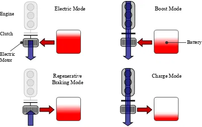
The operation modes describe the operation states of the electric motor and engine. The available modes depend on the powertrain configuration. In the following discussion, only the four operation modes of the considered parallel configuration are introduced (Fig. 1.9). Driving electrically, the clutch between electric motor and engine is open and the vehicle has BEV behaviour. When accelerating, traction power is only delivered by the electric motor (electric mode). When braking, the battery is charged by operating the electric machine in generating mode to regenerate some of the vehicle’s kinetic energy (regenerative braking mode).

Closing the clutch and connecting the engine mechanically to the rest of the powertrain makes two more operating modes available. In boost mode the engine torque is lower than the torque demanded by the driver, and the electric motor supplies the difference. In charge mode the engine torque is higher than the requested torque and the electric machine operates in generating mode to recharge the battery. This enables operation of the engine in high efficiency regions during periods of low cycle power demand, a

Drivetrain Engine Electric Machine Inverter Clutch Charger Battery Electrical Grid Gearbox electric connection mechanical connection (a) Drivetrain Engine Electric Motor Inverter Charger Battery Electrical Grid Gearbox Inverter Generator (b) Drivetrain Engine

Electric Motor Inverter

Charger Battery Electrical Grid Gearbox Inverter Clutch Generator (c) Drivetrain Engine

Electric Motor Inverter

[image:22.595.100.517.145.375.2]

(23)

23

process known as load point shifting (Fig. 1.10). Engine-only operation, corresponding with a conventional powertrain configuration, is referred to as ICE mode.

Frequent switching from boost or charge mode to electric mode should be avoided by the EMS, as this requires starting or stopping the engine and employing the clutch. This results in a higher wear-rate for the clutch and can negatively affect drivability of the vehicle, as the changing vehicle sound is noticeable by the driver. For these transitions an engine start control is necessary which controls motor and engine speed before con-trolling the slip of the clutch [15].

[image:23.595.108.515.238.493.2]

Fig. 1.9. Operation modes of a parallel PHEV. The blue arrows indicate mechanical power transfer, while the red ones indicate electrical power transfer.

Fig. 1.10. Load point shifting. Engine operating points in the specific fuel consumption map.

Electric Mode Boost Mode

Charge Mode Regenerative

Braking Mode

Battery Engine

(24)

24

1.3 Energy Management Problem

Road vehicle speed is controlled by the driver via a positive torque request via the ac-celerator pedal or a negative torque request via the brake pedal. The powertrain control problem of vehicles with conventional powertrains is straightforward, as positive torque is only supplied by the engine. In HEV, a positive torque is supplied either by the en-gine, the electric motor or by both. This difference makes necessary the use of an EMS. The EMS developed in this work is based on the assumption that vehicle speed is con-trolled by the driver by means of a torque control. There are other approaches to EMS which combine power distribution optimization with vehicle speed optimization [16]. Vehicle speed optimization is a method which can increase fuel efficiency in a conven-tional vehicle for a given trip [17].

The tasks of the EMS are distribution of torque demand 𝑇𝑟𝑒𝑞 between electric machine

(𝑇_𝑒𝑚) and engine (𝑇_𝑖𝑐𝑒), gear shifting control, and engine starting and stopping. Optimi-zation of engine torque is usually done in terms of fuel efficiency, but emissions can also be considered. When considering emissions, optimization of the engine operating point is a trade-off principally between nitrogen oxide (NOx) emissions, and fuel effi-ciency [18]. With PHEVs, as a significant portion of the trip can typically be driven electrically, engine emission considerations are, relatively, of less importance with PHEV than HEV. Disregard of emissions considerations is also motivated by practical considerations, as engine emissions are influenced by the transient behaviour of the en-gine; considering emissions resulting from transient engine behaviour would require a more complex dynamic engine model and thus hamper execution in real time.

(25)

25

Fig. 1.11. Communication between EMS and powertrain components.

SOE control depends on whether the battery is rechargeable via the electrical grid or, as in autonomous HEV, only by means of the electric motor operating in generator mode. Therefore, for autonomous HEV the battery energy balance of a trip should be neutral, i.e. the electrical energy consumed by the electric motor should be returned by regenera-tive braking or by using charge mode. This mode of electrical energy use is called charge-sustaining mode (CS). By contrast, the battery in PHEV is preferably recharged via the electrical grid. Therefore, the aim is to deplete the battery across the trip, and recharge it at end of trip. This mode of operation is known as charge-depleting mode (CD). It must be considered that battery recharging times are much greater than refuel-ling times, and recharging during short standstills is not possible.

Fig. 1.12. Energy management problem for PHEV. For trips exceeding the all-electric range, the electrical energy is distributed over the entire trip for highest fuel efficiency.

To achieve charge depletion, two different approaches exist. The simplest implementa-tion is referred to as all-electric mode, which begins the trip driving electrically. At charge depletion corresponding with distance 𝑠𝑒𝑟 (Fig. 1.12), it switches to CS

opera-Drivetrain

Engine Electric Motor

Inverter

Clutch Gearbox

other Signals Driver Signals

EMS

Battery

All-Electric Range

End of Trip Trip Start

Trip Distance s

ser send

(26)

26

tion. This strategy does not necessarily need trip foreknowledge. However, fuel effi-ciency is lower than using blended mode strategies which employ engine use from trip start [21]. The SOC using an AER-focused strategy is depicted in Fig. 1.13, in which the SOC is managed such that it is equal at end of trip and trip start. At second 1117 the all-electric range (here defined when the SOC falls below 0.3) is reached and the engine is started (Fig. 1.15). In contrast, blended mode operation employs the engine from trip start (Fig. 1.16) and restricts engine use to high load trip sections (Fig. 1.18), whereas the all-electric mode has to operate the engine during low load sections in charge mode which causes additional electrical losses (Fig. 1.17). The result is 4.0% lower fuel con-sumption for this cycle using the blended strategy. However, blended CD strategies depend more on the availability of trip prediction data.

Fig. 1.13. SOC during the BCN-CTS cycle using an AER-focused strategy.

Fig. 1.14. SOC during the BCN-CTS cycle using a blended strategy.

(27)

27

Fig. 1.16. Operation modes during the driving cycle BCN-CTS using a blended strategy.

Fig. 1.17. Engine operating points using an AER-focused strategy during BCN-CTS.

Fig. 1.18. Engine operating points using a blended strategy during BCN-CTS.

Focussing on the mathematical formulation of the control problem, the control of en-gine, electric motor, and gear can be simplified to a control of the motor torque 𝑇𝑒𝑚 and

the gear𝑔. The resulting control vector 𝒖 is

𝒖=�𝑇𝑒𝑚_{𝑔 �} . (1.1)

The combustion engine torque 𝑇𝑖𝑐𝑒 can be calculated using the torque demanded by the

driver and the electric motor torque 𝑇𝑒𝑚 using

𝑇𝑖𝑐𝑒= 𝑇𝑟𝑒𝑞 − 𝑇𝑒𝑚 . (1.2)

The engine state 𝑠𝑖𝑐𝑒 refers to whether the engine is running or switched off and is

(28)

28 𝑠𝑖𝑐𝑒 = �

0 engine off

1 engine on , (1.3)

and can be defined with Eq. (1.2) as function of the control vector 𝒖:

𝑠𝑖𝑐𝑒 =�

0 𝑇𝑖𝑐𝑒 = 0

1 𝑇𝑖𝑐𝑒 > 0 .

(1.4)

As engine speed 𝜔_𝑖𝑐𝑒 and motor speed 𝜔_𝑒𝑚 are defined by gear ratio and vehicle speed, the engine and electric motor operating points are entirely defined by 𝒖.

The complexity of the control problem results from two key factors: Firstly, the chal-lenge of solving a predictive fuel efficiency optimization in real time. Secondly, in addi-tion to fuel economy, consideraaddi-tion must be given to engine starts and gear shifts. This explains why engine starts, gear shifting, and complete charge depletion are often ne-glected in literature.

1.4 State of the Art

Owing to the external recharging capability of PHEVs, not all the electrical energy used in their operation must be generated by the powertrain itself. Thus EMS for PHEV dif-fers from other EMS in that it targets CD operation with negative electrical energy bal-ance. Therefore, for minimal fuel consumption PHEVs require predictive strategies which use information about power load and vehicle speed during the future trip. Once the trip destination has been indicated by the driver, using data of a geographic informa-tion system (GIS) the optimal trajectory can be determined using path-finding algo-rithms. From the known trajectory, the navigation system can deliver information about road type, legal speed limits, traffic, maximum possible speeds due to curves, and road grade to a load prediction algorithm which generates a load profile of the trip [22], [23]. Predicted trip speed 𝑣_{𝑐𝑦𝑐𝑙𝑒}, required wheel power 𝑃𝑤ℎ and road grade 𝛼𝑟𝑜𝑎𝑑 are

calcu-lated by the load forecasting algorithm as a function of time (Fig. 1.19).

(29)

29

Fig. 1.19. Information used by load forecasting algorithms for trip prediction.

Many EMS concepts have been already studied; an overview of strategies for HEV can be found in [25] and for PHEV in [26]. EMS approaches can be classified into heuristic and optimization based strategies. Among heuristic strategies are rule-based strategies where operation mode is selected according to “if... then...” rules based on vehicle or engine speed and the power or torque requested by the driver. The rules determine the power distribution such that the operating points of engine and electric motor lie in high efficiency regions [18] and can be designed to imitate optimal behaviour during differ-ent driving cycles calculated using optimization techniques [27]. The rules can also be based on fuzzy logic as presented in [28] for a parallel powertrain, and in [29] for a se-ries PHEV.

While early development of EMS focused on rule-based strategies, recent focus has been on optimization based EMS. Approaches are often based on Pontryagin’s mini-mum principle, which was first used for HEVs [30] and later adapted to the require-ments of PHEVs [31]. Using this strategy, SOC at end of trip depends on the initial conditions chosen for the Lagrange multipliers of the Hamiltonian function, which is minimized to obtain the optimal control policy.

(30)

30

target SOE at end of trip. Therefore, even though the cost function is instantaneous, trip foreknowledge is still required.

Alternative approaches adapt the weighting factor according to SOE development dur-ing vehicle operation by usdur-ing a penalty function [38]–[40]. For PHEV, an online adap-tation of the weighting factor using trip foreknowledge has been presented in [41]. In [42] quadratic programming is used to optimize the weighting factor considering route prediction information with the aim of full battery depletion.

Another common approach, based on the optimality principle of Bellman [43], is time-discrete dynamic programming (DP) [44]. This approach is most often used as a benchmark for other EMS due to its high computational cost [45]. It is used in [46] for a parallel HEV and in [47] for a series HEV. Considering it yields the global optimum with the boundary condition of the SOE at trip start and end of trip, it is also used in combination with stochastic driving cycles for HEV component sizing [48]; deriving rule-based strategies [27]; and training neural networks which imitate the optimization results [49].

Real-time DP implementation in combination with route prediction data has been de-scribed in [50], where measures are taken to reduce DP computational cost (Section 3.2). Another real-time implementation of DP is presented in [34], where gear optimiza-tion is combined with a torque optimizaoptimiza-tion based on Pontryagin’s minimum principle. Stochastic dynamic programming (SDP) can be employed when trip foreknowledge is not known. In [51] this technique is used with stochastic driver power demand gener-ated by a Markov process which is optimized for an infinite time horizon to obtain a time-invariant CS strategy.

In [52] SDP is used for a power-split powertrain configuration to implement both CS and CD operation, using as a cost function the ratio of fuel and the price of electrical energy. Using SDP, it is not possible to determine a target SOC at end of trip as the EMS is generic and is optimized for different driving cycles. SDP is also used in com-bination with Markov chain modelled driving cycles to demonstrate that predictive strategies using trip foreknowledge can reduce fuel consumption in autonomous HEVs [53]. For PHEVs, predictive strategies are even more important, as in order to achieve maximum fuel economy full battery depletion must coincide with end of trip.

(31)

31

powertrain has been used. This fast technique has not yet been used in combination with gear optimization due to the restrictions of linear models. Another technique yielding sub-optimal results is the ℋ∞ control [56], which does not use any a priori knowledge

about speed and power of the future trip.

The above mentioned studies mainly do not consider drivability aspects such as engine start/stop frequency and gear shifting due to the greater complexity of the vehicle model required. In [57] the mechanical energy required to start the engine from standstill to idle speed is considered. Engine start/stop control has been combined with the above described power weighting factor approach for CS operation [57]. In [58] SDP is em-ployed and drivability aspects are included in the cost function. However, as trip fore-knowledge is not used the final SOC cannot be controlled.

In [59] gear shifting losses are considered, and gear shifting limited for a mild hybrid parallel structure. Owing to the challenges of optimizing fuel economy, engine starts and gear shift at low computational cost, the EMS developed in this work considers engine starts and gear shifts indirectly by embedding optimized power distribution and gear shifts within a rule-based strategy.

Optimization results presented are given as torques 𝑇_𝑒𝑚 and 𝑇_𝑖𝑐𝑒 or their ratio. Problems arise when predicted trip data and real values do not coincide due to overtaking maneu-vers, standstill caused by traffic lights, or erroneous traffic information. Erroneous pre-diction data leads to erroneous torque calculations, and consequently vehicle speed does not correspond with the driver’s demand. Using the torque/power ratio instead, vehicle speed is controlled correctly, but resulting torques are no longer optimal. The influence of erroneous prediction data on fuel consumption for a weighting factor based EMS has been evaluated in [60].

1.5 Energy Management Strategy Proposal

Evaluating the existing EMS approaches summarized above, the following requirements for the EMS have been identified:

• use of predictive optimization

• support for charge depletion across the trip using blended mode operation • consideration given to frequency of engine starts and gear shifts

• robustness against inaccurate prediction data.

(32)

32

indicated by the driver), the vehicle speed, acceleration, and road grade 𝛼𝑟𝑜𝑎𝑑 can be

predicted (see Section 1.4).

As the focus is on gear and torque/power control, the trip prediction process is not con-sidered in this study. For EMS development prediction data accuracy is assumed, and in Section 5.8 the robustness of the EMS against inaccurate prediction data is evaluated. Before starting the trip, the first step taken by the EMS is to calculate the optimal power distribution between engine and electric motor for the trip (Chapter 3). Calculation is based on a rapid MILP using a linear vehicle model. From optimal power distribution, the optimal battery power 𝑃𝑏𝑎𝑡 and thus the SOC during the trip are obtained (Fig. 1.13,

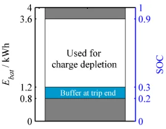
[image:32.595.228.397.428.559.2]

Fig. 1.14). A necessary boundary condition of the optimization is the SOC at end of trip. As depth of discharge significantly effects the battery life cycle, it is recommended that a full discharge is avoided, and instead energy levels are kept within a limited SOC window. The SOC window adopted for this study is 𝑆𝑂𝐶(𝑡)∈[0.2; 0.9]. As the objec-tive of the EMS is to substitute fuel for electrical energy as the power source, at end of trip the EMS should reach full battery depletion. In order to guarantee CS operation without recharging at end of trip, a target SOC of 0.3 is selected. Starting the trip with a fully charged battery, 2.4kWh of electrical energy corresponding to Δ𝑆𝑂𝐶 = 0.6, can be depleted (Fig. 1.20).

Fig. 1.20. Use of stored electrical energy during a trip. The trip is considered to start with the maximum SOC of 0.9. At end of trip a buffer for CS mode remains.

Knowing the optimal 𝑆𝑂𝐶∗₍_𝑡₎_{for the trip and the power}_𝑃

𝑖𝑐𝑒 and𝑃𝑒𝑚, the second step

taken by EMS is to calculate the torque𝑇𝑖𝑐𝑒, 𝑇𝑒𝑚 and the gear 𝑔 .These torques cannot

be directly calculated from 𝑃𝑖𝑐𝑒 and𝑃𝑒𝑚 without knowledge of motor or engine speed,

(33)

33

the trip within a model predictive control (MPC) framework (Fig. 1.21). Computational load undergoes a rise due to the nonlinear vehicle model and the different optimization algorithm required, and therefore an MPC framework using a receding prediction hori-zon is employed.

The SOC boundary conditions of the optimization carried out within the MPC frame-work are given by the function 𝑆𝑂𝐶∗₍_𝑡₎_{, calculated in the first execution process before}

trip start. From this second execution step optimal torque and gear in terms of fuel effi-ciency are obtained. To provide robustness against inaccurate prediction data, results obtained are used to adapt a rule-based strategy online in a final execution step (Chapter 5). To reduce engine start and gear shift frequency, the operation mode is controlled by the rule-based strategy.

The above described approach combines the fuel efficiency of an optimization based strategy with the reduced number of gear shifts and engine starts of a heuristic ap-proach. In the case of inaccuracy of the prediction data, operation in charge mode is controlled by prior calculated electric motor and engine torque lookup tables. The MPC approach is, when using an control horizon of 60s, capable of achieving the desired SOC at end of trip [61]. The EMS presented above can be used for both CS and CD operation. In both cases, results obtained demonstrate near high fuel efficiency, and reduced engine starts and gear shifts, in comparison with the global optimum.

(34)

34

2 Vehicle Model

This chapter discusses, first the characteristics of the exemplary vehicle used in the simulations. Next, the linear and nonlinear model approaches are described, and finally the models are validated with measurements.

The vehicle is a passenger car based on the SEAT Ibiza ST with conventional power-train. To evaluate the EMS developed in the following chapters, fuel and electrical en-ergy consumption of the vehicle is determined by simulating the longitudinal dynamics of this vehicle.

For simulation of fuel and electrical energy consumption, a quasi-stationary approach is sufficient [62]. Simulation of fuel consumption of the engine and electrical energy con-sumption of the electric motor is based on measured fuel mass flow and loss lookup tables, which describe the fuel mass flow and electrical losses in respect to the operating point. Carbon dioxide emissions can be calculated from engine fuel mass flow, their relationship being directly proportional. Other exhaust gases generated by the engine, however, cannot be considered using this approach. For detailed exhaust emissions simulation, a dynamic engine model would be necessary to simulate the engine’s tran-sient behaviour.

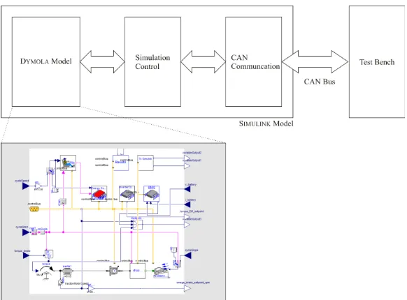
For the different optimization algorithms employed by the EMS proposal, two different vehicle models are necessary. The more complex nonlinear one is in the following re-ferred to as forward model. The modelling approach of the forward model corresponds to a real driving situation: a driver, modelled mainly by a PI controller, acts on the ac-celerator and brake pedal. The inclination of the acac-celerator pedal is translated by the EMS of a HEV, or by the engine control unit (ECU) in conventional vehicles, into a torque or throttle demand for the combustion engine model (Fig. 2.1).

(35)

35

it can, in addition to vehicle fuel consumption simulations, also be used on hardware-in-the-loop (HIL) test benches or for the validation of EMS.

Fig. 2.1. Principle of the vehicle forward model. The driver model controls the pedal variables 𝛼𝑎𝑐𝑐 and 𝛼𝑏𝑟𝑎𝑘𝑒 depending on the driving cycle speed 𝑣𝑐𝑦𝑐𝑙𝑒 and vehicle speed 𝑣.

Fig. 2.2. Principle of the vehicle backward model. Vehicle speed corresponds exactly to the driving cycle speed.

2.1 Vehicle Characteristics

(36)

36

when opening the clutch of a standard ATM is disregarded. Therefore, velocity tracking loss (i.e. the additional power required after shifting and closing the clutch to compen-sate for the interruption) powershifting ATM does not occur [63] and shifting losses are neglected in the powertrain model. The battery with an energy capacity of 4kWh uses Li-ion technology. Its weight is estimated to be 150kg, taking into account mechanical protection and cooling components. When choosing the battery technology (Li-ion, NiMh), in addition to energy and power density [64], the cycle life as a function of the depth of discharge has to be considered. The total energy has to be chosen considering these parameters [65]. The battery can be recharged by operating the electric machine in generating mode or at end of trip by connecting the built-in charger to the electrical grid.

The vehicle base mass corresponds to the vehicle weight of the SEAT Ibiza ST without the engine and transmission and is adapted regarding the additional components of the electric system as indicated in Table II. The sum of the estimated component masses of the hybrid powertrain yields a total vehicle weight including the driver of 1450kg. The complete simulation parameters are indicated in Table III.

Due to direct mechanical connection of engine and electric motor to the wheels, the torque sum 𝑇Σ= 𝑇𝑖𝑐𝑒+𝑇𝑒𝑚 is transmitted to the gearbox input when closing the clutch.

As engine and electric motor speed are equal, the sum of the mechanical power is ap-plied to the transmission. As depicted in Fig. 2.4, the combination of both machines leads to a high maximal torque at every engine/motor shaft speed. As indicated in Fig. 2.5, the available maximal power rises from 98.2kW at 1500min-1_{up to a maximum} power of 130.6kW at 4000min-1_.

Fig. 2.3. Variables of the parallel PHEV powertrain. Drivetrain

Engine Electric Motor Inverter Clutch

Charger Battery

Electric Grid

Gearbox

ωice, Tice

ωwh, Twh

ωem, Treq

electric connection mechanical connection

Pinv,AC

(37)

[image:37.595.92.353.64.411.2]

37 Table II: Estimated vehicle component mass.

Base mass (SEAT Ibiza ST) 950kg

Battery system (4kWh) 150kg

Double clutch transmission (7 speed) 100kg

Engine (3cyl., 51kW) 90kg

Electric motor (80kW) 40kg

[image:37.595.326.520.232.404.2]

Power electronic 40kg

Fig. 2.4. Measured maximal torque of electric

motor, combustion engine and its sum 𝑇𝛴,𝑚𝑎𝑥

at the transmission input.

Fig. 2.5. Measured maximal power of electric

motor, combustion engine and the sum 𝑃𝛴,𝑚𝑎𝑥

at the transmission input.

The specific fuel consumption 𝑚̇_𝑓_,_𝑠𝑝𝑐 of the engine is defined as

𝑚̇𝑓,𝑠𝑝𝑐= 𝑚̇𝑓⁄𝑃𝑖𝑐𝑒 . (2.1)

Minimal specific consumption is reached at a speed of 2000min-1_{and a torque}_𝑇 𝑖𝑐𝑒 >

75Nm (Fig. 2.6). The optimal consumption line depicted is defined as 𝑇𝑖𝑐𝑒,𝑠𝑝𝑐,𝑚𝑖𝑛(𝜔𝑖𝑐𝑒) = arg min_𝑇

𝑖𝑐𝑒

𝑚̇𝑓(𝑇𝑖𝑐𝑒,𝜔𝑖𝑐𝑒)

𝑃𝑖𝑐𝑒(𝑇𝑖𝑐𝑒,𝜔𝑖𝑐𝑒) .

(2.2)

(38)

38 Fig. 2.6. Measured specific fuel consumption map and optimal consumption line 𝑇𝑖𝑐𝑒,𝑠𝑝𝑐,𝑚𝑖𝑛

of the combustion engine.

Fig. 2.7. Measured electric motor efficiency map.

2.2 Simulation Tools

(39)

[image:39.595.96.511.86.496.2]

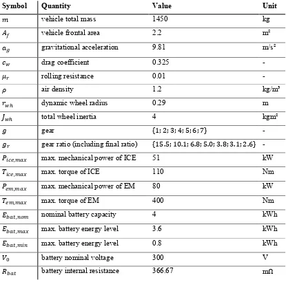
39 Table III: Values of the simulation parameters.

Symbol Quantity Value Unit

𝑚 vehicle total mass 1450 kg

𝐴𝑓 vehicle frontal area 2.2 m²

𝑎𝑔 gravitational acceleration 9.81 m/s²

𝑐𝑤 drag coefficient 0.325 -

𝜇𝑟 rolling resistance 0.01 -

𝜌 air density 1.2 kg/m³

𝑟𝑤ℎ dynamic wheel radius 0.29 m

𝐽𝑤ℎ total wheel inertia 4 kgm²

𝑔 gear {1; 2; 3; 4; 5; 6; 7} -

𝑔𝑟 gear ratio (including final ratio) {15.5; 10.1; 6.8; 5.0; 3.8; 3.1; 2.6} -

𝑃𝑖𝑐𝑒,𝑚𝑎𝑥 max. mechanical power of ICE 51 kW

𝑇𝑖𝑐𝑒,𝑚𝑎𝑥 max. torque of ICE 110 Nm

𝑃𝑒𝑚,𝑚𝑎𝑥 max. mechanical power of EM 80 kW

𝑇𝑒𝑚,𝑚𝑎𝑥 max. torque of EM 400 Nm

𝐸𝑏𝑎𝑡,𝑛𝑜𝑚 nominal battery capacity 4 kWh

𝐸𝑏𝑎𝑡,𝑚𝑎𝑥 max. battery energy level 3.6 kWh

𝐸𝑏𝑎𝑡,𝑚𝑖𝑛 max. battery energy level 0.8 kWh

𝑉0 battery nominal voltage 300 V

𝑅𝑏𝑎𝑡 battery internal resistance 366.67 mΩ

2.3 Quasti-Stationary Nonlinear Model

In this section, a quasi-stationary vehicle model is described. Due to the use of meas-ured consumption tables for engine and electric motor and the non-constant transmis-sion ratio the model is nonlinear. The model is created in the environment MODE-LICA/DYMOLA and used as a forward model for the EMS simulation and its HIL valida-tion. An implementation as a backward model is used by the DP algorithm of Chapter 3. In the backward model, a driver model is omitted assuming that the vehicle speed 𝑣 corresponds at every instance to the driving cycle speed 𝑣_{𝑐𝑦𝑐𝑙𝑒}:

𝑣(𝑡) =𝑣𝑐𝑦𝑐𝑙𝑒(𝑡) . (2.3)

(40)

40

an additional state variable. The vehicle forward model instead includes a driver model based mainly on a PI controller which adapts the accelerator pedal inclination 𝛼_𝑎𝑐𝑐 as a function of the deviation of vehicle speed from cycle speed. The demanded torque 𝑇𝑟𝑒𝑞

by the driver is a function of the pedal inclinations and engine and electric motor speed: 𝑇𝑟𝑒𝑞 = 𝑓𝑟𝑒𝑞(𝛼𝑎𝑐𝑐,𝛼𝑏𝑟𝑎𝑘𝑒,𝜔𝑒𝑚,𝜔𝑖𝑐𝑒) . (2.4)

This control of 𝑇_𝑟𝑒𝑞 by means of a PI controller is required for HIL simulations, as the used ECU does not support torque control. In the following, the components of the for-ward and backfor-ward models are described and differences indicated. While the forfor-ward model is modelled by time continuous equations, the backward model is time discrete. The wheel force 𝐹_𝑤ℎ is calculated as a function of vehicle speed 𝑣 and horizontal road angle 𝛼𝑟𝑜𝑎𝑑 (Table III) by

𝐹𝑤ℎ(𝑣,𝛼𝑟𝑜𝑎𝑑) =𝜇𝑟𝑚𝑎𝑔cos𝛼𝑟𝑜𝑎𝑑+�𝑚+𝐽_𝑟𝑤ℎ 𝑤ℎ2 � 𝑎+

1

2𝜌𝑐𝑤𝐴𝑓𝑣2 +𝑚𝑎𝑔sin𝛼𝑟𝑜𝑎𝑑 ,

(2.5)

where 𝑎_𝑔 is the gravitational acceleration and 𝜌 the air density as indicated in Table III. The wheel torque during the driving cycle is obtained using Eq. (2.5):

𝑇𝑤ℎ(𝑣,𝛼𝑟𝑜𝑎𝑑) =𝐹𝑤ℎ(𝑣,𝛼𝑟𝑜𝑎𝑑) 𝑟𝑤ℎ . (2.6)

With Eq. (2.5), (2.6) and

𝑃𝑤ℎ(𝑣,𝛼𝑟𝑜𝑎𝑑) =𝑇𝑤ℎ(𝑣,𝛼𝑟𝑜𝑎𝑑) 𝑣/𝑟𝑤ℎ (2.7)

results that also the wheel power 𝑃𝑤ℎ transmitted to the wheels corresponds in the

backward model at every instance the cycle power requirement 𝑃_{𝑐𝑦𝑐𝑙𝑒}:

𝑃𝑐𝑦𝑐𝑙𝑒�𝑣𝑐𝑦𝑐𝑙𝑒,𝛼𝑟𝑜𝑎𝑑�=𝑃𝑤ℎ(𝑣,𝛼𝑟𝑜𝑎𝑑) . (2.8)

The torque 𝑇𝑟𝑒𝑞 stands in a direct relation with 𝑇𝑤ℎ as a function of gearbox efficiency

𝜂𝑡𝑟𝑎𝑛𝑠 and gear ratio 𝑔𝑟 (which includes both speed ratio of both gearbox and final

drive):

𝑇𝑟𝑒𝑞 =

⎩ ⎪ ⎨ ⎪ ⎧_𝜂 𝑇𝑤ℎ

𝑡𝑟𝑎𝑛𝑠𝑔𝑟 𝑇𝑤ℎ > 0