Essays on the economics of family formation, dissolution and bargaining

(1)

Essays on the Economics of Family

Formation, Dissolution,

and Bargaining

Pablo A. Brassiolo

TESI DOCTORAL UPF / 2012

DIRECTORA DE LA TESI

Prof. Libertad Gonz´

alez

(2)

(3)

(4)

(5)

Acknowledgments

This dissertation would not have been possible without the help and support from many others. First of all, I would like to thank my advisor, Libertad Gonz´alez, for her constant and generous help, guidance, and encouragement throughout this process. I have been extremely fortunate to have such a great advisor and I am deeply indebted to her.

This dissertation has benefited from useful comments and suggestions from many other faculty members and fellow students, most notably Kurt Schmid-heiny, Patricia Funk, Albrecht Glitz, Gabrielle Fack, Thijs van Rens, Albert Lamarca i Marqu´es, Antonio Ciccone, Christian Fons-Rosen, Rosa Ferrer, Jos´e Garc´ıa-Montalvo, and Federico Todeschini, as well as participants of the Labor, Public, and Development Lunch Seminar at Universitat Pom-peu Fabra. All of them deserve my gratitude for the help in shaping my thinking about the topics presented here.

I also wish to thank Marta Araque and Laura Agust´ı at the GPEFM office for their superb administrative assistance. This research was supported by generous financial aid from the Universitat Pompeu Fabra in the form of a Teaching Fellowship, and the Government of Catalonia in the form of a Research Scholarship.

All these years of research would not have been so enjoyable without the friendship and company of many people at UPF. My gratitude goes to each and every one of them.

Finally, I want to thank my family for their lifetime support, encourage-ment, and love. And special thanks to Vanessa, who experienced all the ups and downs of my research, for all the unconditional love and support she gives me all the time. This accomplishment is also hers.

(6)

(7)

Abstract

This thesis sheds light on several aspects of the economics of marital formation, dissolution, and bargaining. The first chapter focuses on the relationship between divorce law and family wellbeing, and shows that lowering the cost of divorce can reduce spousal conflict. The second chapter analyzes the effects of property di-vision laws upon divorce on marital instability and female labor supply. Results suggest that a redistribution of property rights over family assets in case of divorce towards the financially weaker spouse, usually the wife, may increase marital in-stability and reduce female labor supply. The third chapter examines the role of sex ratios in college in explaining family formation patterns of young adults. Em-pirical evidence suggests that individuals who are exposed to a larger fraction of opposite-sex school mates are more likely to be married or residing with a partner from the same field of study shortly after finishing school.

Resumen

(8)

(9)

Foreword

This dissertation consists of three self-contained chapters that deal with several aspects of the economics of marital formation, dissolution, and bar-gaining. The first two chapters are devoted to improve our understanding of the relationship between family policies and household outcomes, where the effects of those policies on incentives and behaviors play a key role. The main point here is that the rules governing the dissolution of marriages affect the value of the spouses’ outside option, and then, their relative bar-gaining position within the marriage. These changes in the intra-household bargaining position, in turn, are shown to have an effect on the level of family conflict, marital instability, and spouses’ labor supply. The third chapter provides new insights on the functioning of marriage markets. The study examines the role of sex ratios in college in explaining family forma-tion patterns of young adults.

(10)

op-tion. The results are not driven by selection and are robust to a variety of checks.

The second chapter analyzes how the relative bargaining position of spouses affects the incidence of marital dissolution and the labor supply decision of intact couples. The study identifies exogenous variation in bargaining position within the household by exploiting a natural experiment in Spain, where different regions have different rules to divide marital property in case of divorce. This study benefits from two law changes to the separa-tion of property regime in Catalonia, with opposite expected effects on the bargaining position of spouses. Results suggest that a reform that unex-pectedly improved the position of the wife within the marriage increased the divorce rate in around 13 percent in the short run, and although this effect seemed to dissipate over time, it remained positive one decade af-terwards. For intact couples, results show that the same reform caused a reduction in female labor supply of between 0.6 and 2.5 hours per week, and also a reduction in their probability of employment of 2 percent. Moreover, when the previous improvement in wives’ bargaining position was undone by a reform to the scope of marital contracts, female labor supply reacted in the opposite way, with an increase in hours worked and the probability of employment.

The third and final chapter1 _{examines the role of sex ratios in college in}

explaining family formation patterns. Average age at first marriage sug-gests that the initial search for a spouse often takes place before entering the labor market, especially among more educated individuals. This chap-ter studies whether the proportion of classmates of the opposite sex affects the family formation patterns of young adults after finishing their college education. The empirical analysis uses Spanish data, as one of the coun-tries with strong field segregation in college and where high quality data are available on sex ratios by year, field and university. The evidence sug-gests that that sex ratios in college matter. Controlling for labor market

1

(11)

(12)

(13)

1 Domestic Violence and Divorce Law: When

Divorce Threats Become Credible

1.1 Introduction

Domestic violence is an important concern for many societies and policy-makers worldwide. Statistics available for European countries show that between 20 and 25 percent of women have been victims of physical abuse at least once during their adult lives, and around 10 percent have suffered sexual abuse involving the use of force (CAHVIO, 2011). Estimates for the U.S. from the National Violence Against Women Survey show similar num-bers: 1 out of 3 women surveyed reported having been raped or physically assaulted since the age of 18 years (Tjaden and Thoennes, 2000). Moreover, in most of the cases of violence against women, the crime is committed by the intimate partner. In this context, it is natural to ask about the re-lationship between domestic violence and family policies, and specifically, the rules governing the dissolution of marriages. In recent decades, many countries have adopted reforms aiming at simplifying the dissolution of marriage when one of the spouses wants to end the relationship. Since the early 1970s, many states in the U.S. removed fault as a ground for divorce, and almost all of them allowed one of the spouses to file a petition for divorce without the consent of the other. Many European countries have followed similar paths during the past 50 years.

(18)

abuse and divorce legislation, the available empirical evidence in the eco-nomic literature is scarce and shows conflicting results (Dee, 2003; Steven-son and Wolfers, 2006). The relationship between divorce and domestic abuse has also captured the attention of the sociology and criminology literature. However, although alternative theories have been proposed to explain this relationship, empirical research in these fields has, in general, failed to provide credible causal estimates.

This paper studies how divorce law affects domestic violence. It begins by outlining a simple model of bargaining within the marriage to provide a framework for understanding the mechanisms through which easier divorce influences the incidence of spousal violence. The main prediction of the model is that a reduction in the cost of divorce improves the bargaining position of abused spouses by increasing their threat point (i.e. the mini-mum utility level required from the marriage to continue married), and this leads to a lower equilibrium level of spousal violence among intact couples.

(19)

identifica-tion of causal effects. In particular, the effective decline in the length of the dissolution process, and consequently, in the cost of divorce, is limited by the presence of young children, in which case, there are decisions regarding custody and maintenance, which require more time.

This study considers a variety of measures of spousal conflict, ranging from self-reported spousal abuse in surveys and technical definitions of spousal vi-olence based on recorded behavior, to more extreme measures of well-being such as partner homicide. The analysis of the impact on non-extreme mea-sures of violence benefits from a large and rich survey on violence against women conducted in Spain, both before and after the legal change. Besides providing different measures of spousal conflict, these data have allowed knowing the respondent’s marital status at the time of the legal change, avoiding concerns about selection issues. To study the impact on extreme spousal violence, data on female homicide by intimate partner between 2000 and 2010 have been used.

(20)

sug-gests that there is a level of the outside option at which a woman would be indifferent between filing for divorce and continuing in an abusive marriage, and that the impact of the reform should be larger around this margin.1 When using education as an indicator of the outside option, this study has observed larger impacts for women at the center-bottom part of the skill distribution, which indicates that the woman at the margin of indifference has relatively low education.

The results also show a decline in extreme spousal violence, which can be at-tributed to the legal change. Intimate partner homicides of married women have fallen by around 30 percent after the reduction in the cost of divorce. Moreover, a relevant fraction of this decline is explained by a reduction in violence between spouses who are amid a process of marital dissolution. As other social sciences consider marital dissolution as a key determinant of conflict between separating spouses,2 and as both the theoretical frame-work and evidence point to an increase in the share of conflicting divorces (i.e. cases in which one spouse prefers the continuation of the marriage), this result has important implications for the role of the duration of the divorce process. In particular, these findings provide evidence in favor of a negative association between the length of the divorce process and the incidence of ex-spouse victimization.

The literature on the effect of divorce law has focused on a variety of out-comes, such as divorce rates (Peters, 1986; Allen, 1992; Friedberg, 1998; Wolfers, 2006; Gonz´alez and Viitanen, 2009), marriage rates (Rasul, 2006), female labor supply (Gray, 1998; Stevenson, 2008), marriage-specific invest-ments (Stevenson, 2007), fertility decisions (Drewianka, 2008; Alesina and Giuliano, 2006), and children’s outcomes (Gruber, 2004). Less attention has

1

The intuition is straightforward. Women with very poor alternatives outside marriage cannot take advantage of the lower cost of exiting the relationship, while women with very good outside option have a high and credible threat point, independent of the cost of divorce.

2_{See, for instance, Stolzenberg and D’Alessio (2007); Gillis (1996); Campbell (1992);}

(21)

been paid to the effects of unilateral divorce on spousal violence. One ex-ception is the study by Dee (2003), which exploited the variation stemming from the different timing of divorce law reform across states in the U.S. to assess the impact of unilateral divorce on the prevalence of lethal spousal vi-olence. Using state-based panel data from 1968 to 1978, Dee found a small and statistically insignificant effect on the number of wives killed by their husbands, and large and statistically significant positive effects - of around 21 percent - on the number of husbands killed by their wives.3 These re-sults were revisited by Stevenson and Wolfers (2006), who, using the same data source but with a longer panel (1968-1994), found opposite effects on spousal homicide: No impacts on male homicide and a 10-percent decrease in female homicide. Beyond these discrepancies, other concerns made the findings of Stevenson and Wolfers (2006) less than definitive. One is the timing of the effects. As the authors acknowledge, the decline in female homicide predates the legal change to an extent that may undermine their results.4 Moreover, those results are not robust to control for the changes in female homicide committed in unmarried partnerships, which should not be directly affected by the law change.5

In addition, an identification strategy based on variation across time and states could be problematic if both the legal definitions of divorce regimes and reforms introduced vary from one state to another (Mechoulan, 2005; Allen and Gallagher, 2007; Allen, 2007).6 For instance, while many states passed unilateral and no-fault divorce law, some of them require a

separa-3_{Dee (2003) noticed that this effect is driven by states where the treatment of marital}

property favored husbands.

4_{Figure II (p. 285) of their paper clearly shows that the downward trend in female}

homicide started between 7 and 8 years before the adoption of unilateral divorce law.

5_{Using the same database and a similar specification, this study has found a 13-percent}

reduction in intimate partner female homicides among unmarried couples. These results are available upon request.

6_{Other potential problems of this identification strategy is the potential endogeneity}

(22)

tion period, while others do not. Also, those separation requirements may go from a few months to 2 years. In other states, changes in the grounds for divorce were accompanied by changes in property division, alimony, and custody rules. These differences matter. In fact, different coding of divorce regimes is one of the sources of the conflicting findings reached by previous empirical studies.

Stevenson and Wolfers (2006) also studied the impact on non-extreme do-mestic violence, and found that unilateral divorce law caused a reduction in around 30 percent in both female- and male-initiated conflict. The un-fortunate timing of their data, however, prevented them from providing conclusive evidence. The first wave of their data was from 1976, when 31 states had already changed their divorce law, while the second wave was from 1985, when 6 more states had passed that reform. They considered these 37 states as treated and used two alternative control groups - the 9 states that already allowed unilateral divorce in their preexisting regime, and the 5 states that had not passed these reforms by 1985. Thus, their identification strategy relied on a differential evolution in domestic violence between the treatment and control groups, which was then attributed to the reforms. The main problem with this approach is that it may con-found potentially different pre-existing trends in domestic violence between treatment and control states with the true effect of the policy change.7

Research in the sociology and criminology literature has also investigated the relationship between divorce and spousal violence. Some scholars sup-port an “exposure reduction” approach, by which any mechanism that fa-cilitates the dissolution of dysfunctional marriages should alleviate spousal violence by reducing the exposure of the victim to the offender (Dugan, Na-gin, and Rosenfeld, 1999, 2003). Another line of research, however, states that a change towards less effective marital contracts may be ineffective to

7_{Other problems with these results are that 15 states were not sampled in the 1976}

(23)

reduce domestic abuse if it continues between ex-spouses (Campbell, 1992), or even worse, it may intensify it if the abuser feels his or her dominant position is at stake (Wilson and Daly, 1992). Empirical research from these fields, in general, fails to prove causal relationships. For instance, Stolzen-berg and D’Alessio (2007), by examining the cross-sectional relationship between divorce rates and domestic abuse in main U.S. cities, found that cities with higher divorce rates have higher levels of domestic crime be-tween both spouses and ex-spouses. They argued that easier divorce does little to reduce the amount of domestic violence that occurs in a society, because after divorce, abuse continues between ex-spouses. However, they did not consider the potential reverse causality from domestic abuse to di-vorce rates. In a related study, Gillis (1996) used time-series data from 1852 to 1909 from France, and found a strong negative correlation between the rate of marital dissolution and female homicide. However, potential omitted variable bias prevented the author from claiming causation.

(24)

indi-vidual characteristics such as education and the presence of children, among the others. Third, in the analysis of the impact on extreme violence, this study has distinguished female homicide committed by spouses from those crimes involving ex-spouses. This distinction, so far neglected in the eco-nomics literature, is important because easier divorce could affect married and separated couples differently. The results obtained can be interpreted as supportive of an “exposure reduction” approach, because they point out the importance of the shortening of the length of the dissolution process as a key factor explaining the decline in lethal violence against ex-spouses. In this sense, this study also adds to the sociology and criminology literature.

The rest of the paper is structured as follows. Section 1.2 presents a simple theoretical framework for understanding the interaction between divorce law and spousal violence. Section 1.3 describes the main institutional con-text and the identification strategy. The data sources are described in Section 1.4. Section 1.5 presents the main empirical results and, finally, Section 1.6 provides the conclusion.

1.2 Theoretical Framework: Why easier divorce

can affect domestic abuse.

This section presents a simple theoretical framework that attempts to shed light on the interaction between spousal violence and divorce costs. In this model, a marriage is seen as an institution that produces a valuable out-put which is distributed between spouses according to some predetermined shares.8 _{After the marriage has taken place, spouses get to know the utility}

8

(25)

level they would obtain in case of divorce.9 Utility upon divorce is consid-ered as a threat point, since the continuation of the marriage will require that both spouses receive an utility level within marriage at least as high as what they would receive in case of divorce. A key assumption in this model is that those outside options remain private information for each spouse.10

The model has two stages. In the first stage, each spouse observes the value of his or her own utility outside of marriage, and decides whether to continue married or to file for divorce. In absence of mutual consent for dissolution, the spouse seeking divorce has to pay a cost. In the second stage, conditional on the continuation of the marriage, they (re)negotiate about how to distribute the gains of the marriage. A bargaining process is explicitly modeled in this stage, which may involve the use of violence from the husband and may have divorce as a response from the wife.

a A simple model

Stage 1: Realization of payoffs and negotiation to continue the marriage

Individuals make their marriage decision on the base of the expected gains from the union, which are distributed between the partners according to some predetermined shares. Let us denote the utilities within the marriage asuhanduw for the husband and the wife, respectively. Once the marriage

property division after divorce (Chiappori, Fortin, and Lacroix, 2002) may influence individual’s bargaining power in the marriage market. To make the marriage market endogenous to changes in divorce legislation is an important task left for future research.

9_{The assumption of ex-post information about the value of opportunities outside the}

relationship has been motivated in the literature by the arrival of new information during the marriage, such as the value of a potential new relationship or changes in the value of market opportunities (Becker, Landes, and Michael, 1977; Peters, 1986; Weiss and Willis, 1997).

10_{Zhylyevskyy (2008) and Friedberg and Stern (2010) provide empirical evidence}

(26)

has taken place, each spouse observes his or her own outside opportunity, denoted by Ow and Oh, but they do not observe the outside opportunity

of their partner. private information for each of them. Then, each spouse compares the utility levels he or she would receive in each of the states (marriage or divorce), and decides whether to propose the continuation of the marriage or to stand for divorce. When considering the possibility of divorce, each spouse takes into account that the lack of mutual consent for the termination of the marriage implies to pay a certain cost of divorceC.11 On the contrary, if both spouses agree to a divorce, they do not have to pay any divorce cost.12 As a result of individual assessments of utilities in each state, we would have three possible situations:

1. Both spouses prefer divorce: uw < Ow−Canduh < Oh−C. Although

they consider the divorce cost when making the decision, they get mutual consent for divorce and do not have to pay that cost.

2. Both want to continue married: uw > Ow and uh > Oh. There is no

conflict of interest and the marriage continues. Note that in this case the marriage yields a surplus S=uw+uh−(Ow+Oh).13

3. Only one spouse wants to leave the marriage. Assume that the one

11_{There is no distinction in the model between mutual consent and unilateral divorce.}

The regime can be thought as unilateral since any spouse can make the decision of leaving the marriage without having the consent of the other, but incurring in a cost which is not present when there is mutual consent for termination. This setup is motivated in the actual divorce regime in Spain, which allows for unilateral separation based on certain grounds. These grounds include the usual considerations of fault or “de facto” separation, in which case, effective cessation of marital life for a period of 3 years is required. Having to prove fault in court or getting “de facto” separation is the cost that the spouse who wants to leave the marriage unilaterally has to pay.

12_{Notice that a condition for standing for divorce is to be able to afford it, that is:}

ui < Oi−C. Otherwise, if Oi−C < ui < Oi, the person would prefer to continue

married. There will be of course cases in which both would like to get divorced but could not afford it if having to pay C. We can assume with no loss of generality that they would reach an agreement for mutual consent divorce.

13_{Cases in which only one spouse would like to leave the marriage but cannot pay the}

(27)

wanting to get divorce is the wife.14 Two possibilities arise:

(a) She wants to leave and can afford it, but her husband can com-pensate her to stay together: uw < Ow −C and uh −Oh >

Ow−C−uw. I assume that if compensation is possible,

what-ever the scheme of this compensation is, the compensation takes place and the marriage continues.15

(b) She wants to leave and can afford it, and her husband cannot compensate her to stay together: uw < Ow−C and uh−Oh <

Ow−C−uw. Compensation is not feasible and there is divorce.

Note that the husband would prefer to continue married but can not convince her to stay. The dissolution is unavoidable and conflict may arise with the decision of the wife of leaving the relationship.

Stage 2: (Re)negotiation of the distribution of gains of marriage

Conditional on the continuation of the marriage, spouses may (re)negotiate the distribution of the marital surplus. Marriages that survive the first stage are: (i) those in which both spouses want to stay married, (ii) those in which one spouse wanted to leave but was compensated by the other to stay together. To simplify, assume that renegotiation only takes place in case (i). Note that the surplus S is not known with certainty, since the outside option of the other partner is not observable.

Assume now that the husband can force a renegotiation of the distribution of the surplus in order to maximize his value of the marriage, and this renegotiation requires the use of violence. He can either choose violence (V) to claim a transfer (T(V) =T) from his wife, or choose no violence (N V)

14

The case in which it is the husband instead, is completely symmetric.

15_{Note that the existence of divorce costs may imply that some inefficient marriages}

(28)

and remain with his original share of the surplus (that is, T(N V) = 0).16 If he chooses violence and there is no divorce, his utility becomesuh+T.17

The wife responds by deciding whether to stay in the marriage, accepting a lower share of the surplus (because of the transfer and the disutility from violence), or to file for divorce. If she stays, her utility is uw −T −Vw,

whereVw is the disutility from violence. If she divorces, her utility is given

by Ow−C.

Wives differ in their outside option, such that Ow ∼ [Ominw , Omaxw ]. We

can interpret this as their labor market potential after divorce or their remarrying probabilities.18 The husband does not know the true value of Ow, but only the distribution in the population.

The solution for the second stage of the game can be found by backward induction. The wife will choose between staying and leaving, given the decision of her husband. In the absence of violence her best strategy is to stay, given that uw > Ow −C for all women in this stage. If there is

violence, she will divorce if and only ifOw−C > uw−Vw−T. Otherwise,

she will stay in the marriage and suffer violence from her husband.19 The husband makes his decision about violence knowing only the probability that she will divorce if her utility inside marriage falls below the value of her outside option. To simplify the notation, let us call p the probability

16

This transfer should be interpreted as any redistribution of the gains of the union in favor of the husband.

17

This would imply that violence is “instrumental”, in the sense that it is used as a means to get a higher share of S.

18

In order to have that some wives would divorce in case of violence and others do not, we need to impose some restrictions to the distribution of Ow, such as: Omaxw −C >

uw−Vw−T andOwmin−C < uw−Vw−T.

19

(29)

that she will divorce as a consequence of violence.20 Then, he compares the extra utility he would receive if violence is accepted with the probability that she divorces and he is being left with his outside option. A condition for choosing violence, therefore, is that (uh+T)(1−p) +Ohp > uh. If this

inequality holds, the husband will choose violence; and the wife will stay in an abusive marriage with probability 1−p=FOw[uw−Vw−T +C], and

divorce with probabilityp= 1−FOw[uw−Vw−T +C].

b Comparative Statics and Implications

This simple model yields clear and intuitive predictions on the impact of a reduction in divorce costs on domestic abuse. The probability of domestic violence is: FOw[uw−Vw−T+C]. This is increasing in the cost of divorce,

C, which leads to the following proposition:

Proposition 1 The prevalence of domestic abuse among married couples decreases after the reduction in the cost of divorce.

It is important to notice that the reduction in domestic violence comes not only from the increase in dissolutions of abusive marriages, but also from a reduction in the incentives of husbands to choose violence. To see this more clearly, the condition for the husband to choose violence can be rewritten like this:

T(1−p)>(uh−Oh)p

If the reform changes the probability p, it also changes the incentives to choose violence in order to force a renegotiation of the surplus. The reform,

20

A wife will leave an abusive marriage if she has a good enough outside option, that is: p=P r(Ow−C > uw−Vw−T) = 1−FOw[uw−Vw−T+C], whereFOwis the c.d.f.

(30)

therefore, reduces the equilibrium level of domestic violence through an improvement of the bargaining position of the wife.

The model has also implications for the distribution of the effects in terms of individual characteristics. One of the main sources of heterogeneous responses to changes in divorce law is the presence and age of children. This argument can be rationalized at least in two ways. First, the reduction in the cost of divorce is larger for women without children under age 18. Having young children lengthen the divorce process since decisions about custody and maintenance payments have to be made. Second, the presence of young children has been found an important determinant of individual-specific cost of divorce (Del Boca and Flinn, 1995; Weiss and Willis, 1997). For instance, mothers of young children are likely to face higher emotional and economic costs of marital dissolution than non-mothers or mothers of older children. A simple extension of the model would be to assume that the cost of divorce for a certain woman,Cw, depends not only on the divorce

cost determined by the current legal regime, say C, but also on individual characteristics, cw. While the reform in divorce law affects the general

component of the cost of divorce, the presence of an specific component will lead to differences in the intensity of the treatment.

Corollary 1 The reduction in the incidence of abuse is larger for women more affected by the reduction in divorce cost.

A second source of heterogeneous responses to the law change are differences in women’s outside option. The following corollary shows this:

Corollary 2 The reduction in the incidence of abuse is larger for women with better outside options.

(31)

domestic abuse should come not from women at the top end of that distri-bution, but from women with better outside of marriage prospects among those suffering abuse in the old regime. Figure 1.1 illustrates this point.

In this model, divorce happens in equilibrium not only as a response to spousal violence in the second stage but also as a consequence of realizations of outside options (net of divorce cost) in the first stage. The reduction in the cost of divorce, then, will affect the probability of divorce. In particular, it will increase the frequency of divorces in which one spouse prefers the continuation of the marriage.21

Proposition 2 The rate of non-mutual consent divorce increases after the reform in divorce law.

How is this related to spousal violence? As the sociology and criminology literature show, partner violence -and in particular, extreme violence- of-ten occurs around important events in a relationship such as a unilateral breakup decision (Stolzenberg and D’Alessio, 2007; Wilson and Daly, 1992; Campbell, 1992). The reduction in the cost of divorce would lead to a higher demand for divorce and, in particular, a higher share of unilateral breakups, which could potentially lead to more conflict between separating spouses. At the same time, the legal change shortens the length of the whole dissolution process, from the decision to divorce until divorce is effectively obtained. Therefore, assuming that the highest risk of spousal violence occurs during the dissolution process, whether we should expect more or less violence between separating spouses would depend on which effect pre-dominates: the increase in the number of spouses involved in conflicting dissolution or the reduction in the length of time required to dissolve the marriage. For instance, ifN is the number of couples,dis the probability of divorce,h is the probability that a divorce ends in partner homicide during the divorce process (per unit of time at conflict), and t is the duration of

21_{The reduction in the cost of divorce makes it more difficult for the spouse who values}

(32)

that process, the number of partner homicides between separating spouses is: N∗d∗t∗h. Suppose now that a reform of divorce law makes: d1 > d0

andt1 < t0, where 0 and 1 denote the pre- and post-reform period,

respec-tively. Suppose also that N and h are unchanged by the reform.22 Then, at a certain point in time during the new regime, the number of people at risk of spousal homicide will be lower if and only if d1/d0 < t0/t1.

1.3 Empirical Strategy

a The Reform of Divorce Legislation in Spain in 2005

In July 2005, the Spanish parliament approved a comprehensive reform of the rules governing marital dissolution in Spain.23 This reform included two key modifications that substantially lowered the barriers to divorce. First, it eliminated the mandatory 1-year legal separation period before divorce.24 Second, it allowed for unilateral and no-fault divorce.25 As a consequence of these legal changes, the divorce regime suddenly went from one with fault and mandatory separation period to another with easy, unilateral, and no-fault divorce, dramatically reducing both the economic and emotional costs of marital dissolution.

The old regime, which was in place since 1981, was mainly characterized by a two-step process to deal with marital breakdown. The couple who wanted to dissolve the marriage generally had to resort to a period of separation

22

Sincehis the probability of spousal homicide during the divorce process per unit of time at conflict, it can be assumed as unchanged by the reform.

23

Act 15/2005 of July 8th, modifying the Spanish Civil Code and the Civil Procedure Rules on matters of separation and divorce.

24_{Legal separation is left as an option for those not wanting to resort to divorce.} 25

(33)

before being able to file for divorce.26 Once the petition for legal separation had been filed, at least 1 year had to pass before filing for divorce. Sep-aration, in turn, could be obtained by mutual consent or unilaterally, but based on a legal ground. The legal grounds for separation established in the Spanish Civil Code included the usual considerations of fault - unjustified abandonment of the family house, marital infidelity, abusive conduct, being sentenced, alcoholism, drugs addiction, etc. - or the effective cessation of marital life for a period of 3 years.27

The combination of unilateral and no-fault divorce with the possibility of fil-ing for divorce directly, without legal separation as a necessary step, implied a substantial reduction in the length of time needed to obtain a divorce. Quantifying this time reduction is not an easy task, because it may depend on whether there was mutual consent for separation or not, and on the ground on which separation was based. A lower bound for this shortening of the process can be determined in 1 year, the period established in the old regime between the separation petition and the possibility of initiating the divorce process. Nevertheless, in some cases, this period can be much longer, particularly in those relationships in which there was no mutual consent for termination. The old regime made separation particularly dif-ficult for a spouse who was unhappy in a relationship and wanted to leave without having the consent of the other partner. A person like this usually faced two alternatives. One was to go to court and claim separation on the base of fault, in case it existed, which may involve a lengthy and expensive legal battle with the other partner. A second alternative consisted of stop-ping marital life for a period of 3 years, and then claim legal separation on the base of de facto separation. In such a case, the change to

unilat-26

There is one exception in which it is possible to directly file for divorce, which cor-responds to the case in which there is risk of violence against the spouse or the children. For a more detailed description of the grounds for divorce in Spain before the reform of 2005 see Boele-Woelki, Braat, and Sumner (2003)

27_{This length corresponds to the case in which the cessation of marital life is not}

(34)

eral and direct divorce may imply a reduction to the dissolution process of about 4 years (3 years to file for legal separation on the ground of de facto

separation plus 1 year before being able to file for divorce).28

As a consequence of the relaxation of the requirements to obtain a divorce, there was a huge increase in the number of divorce proceedings petitioned. Figure 1.2 shows the evolution of marital dissolution in Spain between 1975 and 2010. In the first year after the reform, the number of divorce petitions that entered into local courts increased by 170 percent. This was only partially compensated by a decline in separations, which can be explained by the fact that legal separations remain only as an option for those who do not want to opt for divorce directly.

Besides this increase in the number of marital dissolutions, the law change may have had a differential effect on women and men. For instance, in the old regime, women were more constrained than men to exit a relationship due to high costs of obtaining a divorce. The analysis of who is the spouse filing a petition for the dissolution of the marriage points to this direction. A separation or a divorce can be petitioned by one of the spouses or by both. Figure 1.3 shows the evolution of separations in which only one spouse has filed the petition, while Figure 1.4 shows the same for divorce proceedings.29 In both cases, it is possible to observe an increase in the proportion of dissolutions initiated by wives after the reform, which provides evidence supporting the hypothesis that women are more benefited by the reduction in divorce costs.

28

It is important to note that this is only an upper bound and, probably, in many cases, it would not be reached, even if it is not possible to prove that the other spouse has incurred any of the typified grounds for separation. This is because in those cases, courts usually refer to the so-called “lack of affectio-maritalis” as a valid ground for separation (Boele-Woelki, Braat, and Sumner, 2003).

29

(35)

Other legal changes regarding domestic violence in Spain

During the period covered by this study, two integral plans and one main law aimed at preventing and combating domestic abuse were implemented. The First Action Plan against Gender Violence (1998-2001) and the Second Integral Plan against Domestic Violence (2002-2004) were elaborated and implemented by the Spanish Women’s Institute. Those plans mainly in-cluded measures aimed at fostering awareness and prevention for potential victims, increasing the availability of resources for victims, and augmenting sanctions for aggressors. A major landmark in the fight against domestic violence, though, was the introduction in December 2004 of an integral law providing comprehensive protection measures against gender-based vi-olence.30 These measures can be grouped into three broad areas of inter-vention. The first consists of awareness-raising and prevention measures on the one hand, and education and training activities on the other hand. The main measures involve informational campaigns, raising-awareness adver-tising in the media, reinforcing the notion of equality of rights and oppor-tunities between men and women in school curricula at all levels, training of healthcare professionals in detecting and preventing violence, and train-ing of legal protection and support professionals. A second group includes penal and judicial measures such as increased penalties for gender-based of-fenses and the establishment of specialized courts to deal with this kind of crimes. Finally, the third group of measures aims at increasing protection for victims of gender violence.

b Identification Strategy

The identification strategy is essentially based on the reform in divorce legislation that took place in Spain in 2005, which can be considered as a source of exogenous variation in the rules of the game regarding marriage dissolution. As such, this reform constitutes a natural experiment and then provides a unique opportunity to identify the causal effect of easier divorce

30

(36)

on domestic violence.

Two basic conditions should fulfill this legal change to constitute a valid natural experiment: being unanticipated and exogenous to the evolution of domestic violence. There are reasons to believe that these conditions are guaranteed. With respect to the first point, the reform in divorce legislation was part of a series of legislative measures concerning family law introduced by the Socialist Party right after winning the general elections in March 2004. The reason why these legal changes can be considered unexpected is that the election results themselves were totally unexpected. Until shortly before the national elections to the Spanish parliament were to take place, the incumbent party held a majority of public support according to avail-able forecasts.31 But a large-scale terrorist attack that hit the commuter train system in Madrid just 3 days before the date of the election suddenly changed the election outcome and resulted in a surprising victory of the op-position Socialist Party (Montalvo, 2010; Bali, 2007; Colomer, 2005; Chari, 2004).

With regard to the exogeneity of the legal change with respect to domestic violence, the stated purpose of the law was to give to the spouses the freedom to decide whether they want to continue married or not, and to eliminate the double procedure (fist separation and then divorce) usually needed to end a marriage, reducing both economic and emotional costs of marital disruption.

Then, the identification strategy used in this paper relies on a difference-in-differences approach (Angrist and Krueger, 1999; Heckman, Lalonde, and Smith, 1999), using married couples as the treatment group and cohabiting partners and individuals in a relationship but not legally married as a con-trol group. That is, I compare the change in spousal violence for married women before and after the reform in divorce law, to the change in spousal violence for women not directly affected by the legal change (i.e. those in a relationship but not legally married). In this way, this empirical framework

31

(37)

allows to control for systematic differences in the level of domestic violence both between married and unmarried women and between before and after the law change.

More formally, if Y1 denotes the outcome of interest with treatment and

Y0 without, t0 and t denote the pre- and post-treatment periods, and D

is a binary indicator of program participation, the difference-in-differences estimator can be written as follows:32

∆DiD= [Y1t−Y0t0|D= 1]−[Y₀_t−Y₀_t0|D= 0] (1.1)

Since it is not possible to observe Y1 and Y0 for the same individual at the

same time, this estimator relies on the following identifying assumption:

E[Y0t−Y0t0|D= 1] =E[Y₀_t−Y₀_t0|D= 0] (1.2)

which is known as the common-trends assumption and requires that both the treatment and the control groups would have followed the same trend in the outcome variable, absent any reform. Under this assumption, it is possible to use the evolution of the population average difference over time in the control group as a benchmark to estimate the treatment effects. In terms of married and unmarried populations, this implies that the mean effect of the reform on spousal violence can be obtained as follows:

∆AT T = [E(Yit|M arried)−E(Yit0|M arried)]−

[E(Yit|U nmarried)−E(Yit0|U nmarried)] (1.3)

whereY denotes some measure of spousal violence.

32

(38)

Although there is no formal test to check the assumption of common trends between the treatment and control group, there are different ways to inves-tigate its validity. The most straightforward is by graphically examining the data and comparing the trends of both groups in the pre-treatment period. An alternative test is to add controls for potentially different group-specific trends in the regressions and investigate whether there is enough evidence to reject the equal trends assumption. Both tests are carried out in the empirical analysis.

One potential threat to the validity of this assumption comes from aggre-gated shocks that have a differential impact across treatment and control groups. This may happen if the unobserved differences between both groups are correlated with those shocks. A potential candidate to constitute such a shock is the approval of the Law Against Gender Violence at the end of 2004. Nonetheless, most of the measures for protection against gender violence are aimed at all women, regardless of marital status. The only exception is given by measures aimed at facilitating separation and divorce procedures in cases in which domestic violence is alleged.33 But even in the case that these measures have a differential impact between married and unmarried women, this effect would be intrinsically related to the main purpose of this paper, which is to assess the impact of easier divorce on the level of domestic violence.

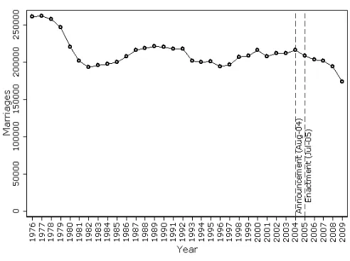
Another key assumption of the difference-in-differences estimator is that there are no changes in the composition of the groups as a consequence of the reform. Otherwise, coefficients would be biased. To test the validity of this assumption, I use microdata from the census of marriages to evaluate two potential concerns in relation to the reform in divorce legislation. First,

33_{The Law Against Gender Violence of 2004 created specialized courtrooms to deal}

(39)

I test whether there is evidence of a structural break in the time-series of marriages. Second, I check for potential changes in the composition of those who marry after the reform.

c Specifications

Non-extreme violence

The difference-in-differences approach translates into the following specifi-cation, in order to estimate the impact of easier divorce on non-extreme spousal violence:

DVigt=β0+β1M arriedg+β2(M arriedg∗P ostt)+

X

t

λtY eart+Xigt0 γ+µigt

(1.4)

where DVigt is a measure of domestic violence for individual i, marital

group g, and year t, M arriedg is an indicator of the treatment group,

P ostt is a binary indicator for the post reform period and therefore β2 is

the difference-in-differences estimator.

(40)

over time, the same definition is used for years 1999 and 2002.

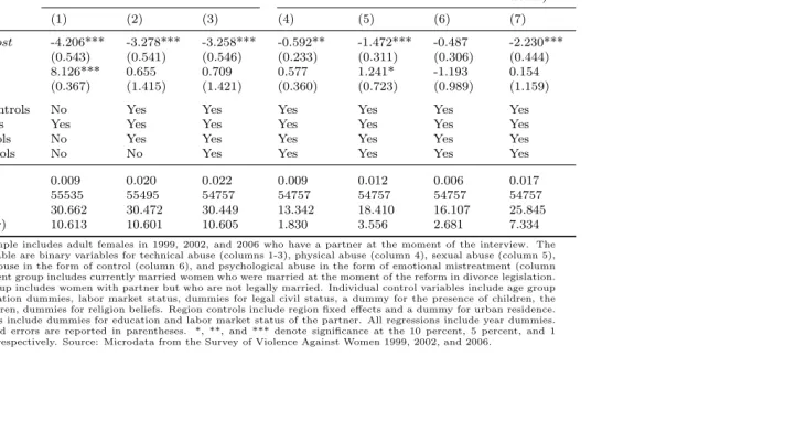
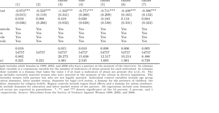
There are two main measures of non-extreme domestic violence to be used as dependent variable. The first is a measure of self-reported abuse and is based on the interviewee’s perception of having been victim of abuse from her intimate partner. The variable is defined as a binary indicator which takes value 1 if the woman reports abuse from intimate partner during the previous year. The second measure is called “technical abuse”, since it is based on a series of 13 questions referred to behaviors or situations which are considered by experts as strong indicators of mistreatment. The survey contains information about the frequency with which these situations occur (i.e. frequently, sometimes, rarely, never) and about who is the offender. “Technical abuse” is a binary variable that takes value 1 if any of these 13 indicators occurs “frequently” or “sometimes” and the offender is the inti-mate partner of the victim. Also, this second measure can be disaggregated into four additional measures of abuse -physical, sexual, psychological in the form of control, and psychological in the form of emotional mistreatment, according to a classification elaborated by Alberdi and Matas (2002). In the tables below I consider these definitions of violence as alternative out-comes. The details of the construction of these measures as well as the description of the 13 indicators of abuse and the corresponding sampling frequencies are reported in Table A1.1.

These different measures of abuse lead to different sample definitions. On the one hand, when the dependent variable is self-reported abuse, since this information is available for all surveyed women, the sample includes all women who were in a relationship during the previous year. On the other hand, when the dependent variable is a measure of technical abuse, since that information is only available for women who are in a relationship at the moment of the survey, the sample is restricted to women who fulfil that condition.

Finally, the vectorXigt includes a rich set of control variables that can affect

(41)

includes control variables for woman’s age, education, labor market status, presence and number of children, religion beliefs, urban-rural residence, and region fixed effects. In some specifications, this vector also contains controls for education and labor market status of the partner.

Extreme violence

I estimate the following equation to capture the impact of the law change on female homicide:

F Hgqt = β0+β1M arriedgqt+β2(M arriedgqt∗P ostqt) +

X

q

γqQuarterq+

X

t

λtY eart+µgqt (1.5)

where F Hgqt refers to female homicides by intimate partner for group g,

quarterq, and yeart. In a first stage, the treatment group includes married and separated women, while the control is conformed of unmarried women. The reason to include both spouses and ex-spouses in the treatment group is that we are interested in the effect of easier divorce on spousal violence and we want to be sure that a potential effect on still married couples is not the consequence of the displacement of violence from married to separated couples.34 In a second stage, I decompose the treatment group into two subgroups: Those victims who were still married and those who were already separated:

34

(42)

F Hgqt = β0+β1Stillmarriedgqt+β2Separatedgqt+

β3(Stillmarriedgqt∗P ostqt) +β4(Separatedgqt∗P ostqt) +

X

q

γqQuarterq+

X

t

λtY eart+µgqt (1.6)

The dependent variable is a measure of female homicides committed by in-timate partner. It can be defined in at least three alternative ways, which lead to different econometric specifications. The first alternative, and prob-ably the most natural, is to define it as a count. I use the aggregate number of intimate partner female homicides by marital status and quarter, for the period between 2000 and 2010. When the dependent variable is defined as a count, it is natural to assume it follows a Poisson process. Then, following the conventional parametrization of this kind of model, this implies that ln(λgqt) =Xgqt0 β, where Xgqt0 is a vector of explanatory variables andλgqt

is the conditional mean of the number of homicides per group and period.35

An interesting property of Poisson regression models is that we can use individual or grouped data, with equivalent results. The only practical implication when using grouped data is that we need to include the log-arithm of the population size for each group among the explanatory vari-ables. On the other hand, one well-known limitation of Poisson models is the equidispersion property, by which the mean is equal to the variance (i.e. E(F Hgqt) =var(F Hgqt) =λgqt). This means that the usual

assump-tion of homoscedasticity is not appropriate. The simplest way in which this concern can be addressed is by obtaining a robust estimate of the variance-covariance matrix of the estimator. Alternatively, the Negative Binomial regression model can be used, since it allows for overdispersed data (Cameron and Trivedi, 2005).

35

This specification assumes that the number of homicides per groupgand period of time given byq andt, F Hgqt, has a probability mass function equal to: pr(F Hgqt) =

λF Hgqt

(43)

A second alternative is to convert the count into a rate, by dividing the number of homicides by the corresponding group population size estimate, and estimate the model by OLS.36 The choice of the functional form is not trivial. In fact, one of the reasons behind the conflicting results of past empirical studies is the use of different functional form. Then, investigating the stability of the results under different specifications is a way of assessing the robustness of those results.

The third alternative for the definition of the dependent variable consists of using the logarithm (instead of the level) of the homicide rate, in which case OLS is an appropriate model as well. The reason for this is that the homicide rate is always positive and therefore a linear model for the logarithm of the homicide rate is a more natural alternative (Lee and Solon, 2011).37

The main coefficient of interest is that of the interaction between the indi-cator of the treatment group and the dummy for the post reform period. This coefficient gives the average change over the post reform period in intimate partner homicide attributable to the law change.

In all cases I run the regressions with year and quarter fixed effects. In some cases, I also include linear group-specific time trends, in order to investigate the robustness of the results to the possibility that the common trends assumption fails.

Finally, there are two possibilities to define the beginning of the post reform period: to consider the date of announcement or the date of enactment. The law was approved by the Spanish parliament in July 2005 and was in force since that date, but was announced around 10 months earlier, when the first bill was approved by the Council of Ministers and submitted to the

36

Population sizes for different marital groups can be obtained from the Spanish Labor Force Survey on a quarterly basis.

37

(44)

Congress.38 Since individuals may react to the introduction of new divorce regime right after its announcement, the post-reform dummy P ostqt is set

equal to 1 since the third quarter of 2004.39 The empirical results shown in Section 1.5, however, are robust to using either date as the beginning of the post reform period.

Marital dissolution

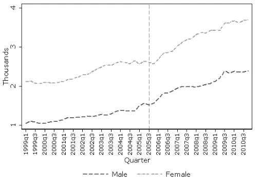
Easier divorce can affect the incidence of domestic abuse by easing the dissolution of abusive relationships. Therefore, to complete the empirical analysis we need to assess the impact of the law change on marital disso-lution. Evaluating this by looking at divorce rates directly is problematic, since the nature of the reform makes the before-after comparison mean-ingless.40 _{To overcome this, I assess the impact of the reform on marital}

dissolution indirectly, by looking at the evolution of the stock of divorcees. The share of divorcees in the population at a point in time depends on both

38_{The whole process of approval of the legal change was actively followed by the}

media. To the best of my knowledge, the first newspaper article anticipating the reform to be introduced appeared on August 17th, 2004, in El Mundo newspa-per (http://www.elmundo.es/elmundo/2004/08/17/espana/1092742690.html). After the Council of Ministers passed the first bill, it was first approved by the Congress of Deputies in April 2005, and later by the Senate in June 2005. The final enactment day was July 8th, 2005.

39

The hypothesis that individuals became aware of the new policy around its an-nouncement is supported by evidence provided by the search intensity on the internet for information about the legal change. This is shown by Figure A1.2, which depicts the evolution of the search intensity for the querydivorcio-the Spanish word for divorce- in the search engine Google. There were two peaks in the search intensity for this query, coinciding with the announcement and enactment dates of the legal change. These data can be obtained at http://www.google.com/insights/search.

40

(45)

the propensity to divorce (the flow into divorce state) and the probability of remarrying (the flow out from divorce state). Then, abstracting from changes in remarriage rates, the evolution of the stock of divorced individ-uals can shed light on the impact of the reform on divorce probability.

To perform the analysis, I rely on data from the Spanish Labor Force Sur-vey, which allows to construct fairly precise estimates of population size by marital status, on a quarterly basis. I use the stock of separated and divorced individuals -for simplicity I refer to this group as to divorcees- to estimate the following equation:41

divorceeit = β0+β1timet+β2post2005t +β3timepostt+

X_it0γ+X

q

λqQuarterq+µit (1.7)

where divorceeit is a dummy variable set equal to 1 if individual i is

sep-arated or divorced at time t, timeis a continuous variable indicating time in quarters from the start of the observation period, post2005 is a dummy that equals 1 since the third quarter of 2005, when the reform in divorce legislation became effective, andtimepostis a continuous variable counting the number of periods after the law change. This flexible specification al-lows the stock of divorcees to trend linearly with potentially different slopes before and after the reform, and to have a change in level that can be at-tributed to the reform. That is, β2 estimates the level change in the stock

of divorcees immediately after the reform, whileβ3 estimates the change in

the trend in the mean number of divorcees after the reform. The vector of control variables, X_it0 , includes dummies for age and education groups, and also a dummy for gender when both men and women are included in the

41_{The survey does not distinguish between separated and divorced individuals, but this}

(46)

sample. Since I use quarterly data, quarter fixed effects are also added to control for seasonality.

Marital formation

The validity of the difference-in-differences approach proposed to estimate the impact of easier divorce on domestic violence requires that the reform neither affected the propensity to marry in the population nor the compo-sition of those who marry. I test to what extent these two assumptions are supported by the data by using data on marriage records.

First, to investigate the possibility of a structural break in the series of marriages after the reform in divorce law, I estimate the following model using monthly data:

marriagest = β0+β1timet+β2post2005t +β3timepostt+

β4marriagest−1+β5GDP growtht−12+ X

t

λtmontht+µt (1.8)

where the dependent variable,marriagest, is the number of new marriages

in month t, time is a continuous variable indexing the month; post2005 is the usual indicator for the post-reform period, and timepost is a continu-ous variable indicating time since the introduction of the reform. Variables marriagest−1 and GDP growtht−12 are included to control for

autocorre-lation and for the influence of economic conditions on the propensity to marry.42

Second, to investigate potential changes in the composition of new couples, I estimate the following equation:

42

(47)

charit=β0+β1timet+β2post2005t +β3timepostt+

X

t

λtmontht+µit (1.9)

where charit is a dummy variable that takes the value 1 if the individual

i who gets married in month t has a particular observable characteristic and 0 otherwise, and post2005t is set equal to 1 since July 2005. The

observable characteristics considered are spouses’ main occupation, age at marriage, and previous legal civil status. As before, time and timepost are two continuous variables indicating time in months at time t, the first counting from the start of the observation period and the second from the enactment of the reform.

1.4 Data and Descriptives

a Databases

I employ two main databases to conduct the empirical analysis: a nationally representative survey on violence against women, and the official registry of female homicides by intimate partners.

Survey on Violence Against Women

To study the effects on non-extreme violence, I rely on microdata from the Survey on Violence Against Women conducted by the Spanish Women’s Institute in 1999, 2002, and 2006. This survey is representative of all adult women (age 18 or older) living in Spain, irrespective of whether they are in a relationship or not.

(48)

construct the measures of self-reported as well as technical abuse mentioned before. Respondents to the survey were queried about whether they think they have been victims of abuse from their intimate partner during the pre-vious year and at any time in their adult life. They were also asked detailed questions about a series of situations considered indicators of violence, the frequency of this happening, and their relationship to the perpetrator.

The questionnaire also included detailed questions regarding the partner-ship status of the respondent, which allows to distinguish up to seven differ-ent marital groups: married, cohabiting, legally separated, divorced, widow, dating, and single. There is also information on the duration of the relation-ship. In addition, the survey also provides information -both for the woman and for her partner in case she has one- on demographic characteristics, la-bor market status, educational background, and household composition.

Data on female homicide by intimate partner

To study the impact of the reform on lethal spousal violence, I use data on female homicides by their intimate partner for the period between 2000 and 2010. Intimate partners include current and former husbands, opposite-sex cohabiting partners, boyfriends, and dates. There are two different sources for these data. The Spanish Women’s Institute, an autonomous body at-tached to the Ministry of Health, Social Policy, and Equality; provides infor-mation on the annual number of fatal victims of intimate partner violence, disaggregated by victim-perpetrator relationship.43 The Queen Sofia Cen-ter (QSC hereafCen-ter), a non-governmental institution devoted to the study of violence, provides similar information but on a monthly basis and with more details about the crime.44 Besides knowing the victim-perpetrator relationship, QSC’s data provide information about age for both of them,

43_{Their sources of data are the media and the Ministry of the Interior for 2000-2005,}

and the Government Office on Gender-based Violence for 2006-2010.

44_{Data come from the Ministry of the Interior, the media, and the courts responsible}

(49)

place of residence of the victim, place where the crime was committed, and the motherhood status of the victim. For women who were legally married at the moment of the homicide, there is also information on whether the they had initiated the procedure to obtain legal separation. Because of the more detailed information and the possibility of defining the pre- and post-reform period with precision given the availability of data on a monthly basis, most of the empirical analysis below is based on QSC’s information.

One limitation of both databases is that they do not distinguish between legally separated and already divorced victims in cases in which the per-petrator is the former spouse. In those cases, the victim-perper-petrator rela-tionship is coded as “ex-spouse”. The importance of that differentiation is that while separated partners are affected by the legal reform (i.e. their dissolution process is subject to the new regime), those already divorced are not. This shortcoming of the data, however, appears to have little prac-tical relevance. Both information contained in cases’ description in QSC’s data and anecdotal evidence seem to point to a majority of those cases corresponding to parters amid a process of separation and, therefore, not yet legally divorced.

Other sources of data

(50)

b Sample Definition and Descriptive Statistics

This section presents the basic features of the data used in the empirical analysis.

Non-Extreme Violence: Self-reported and Technical Abuse

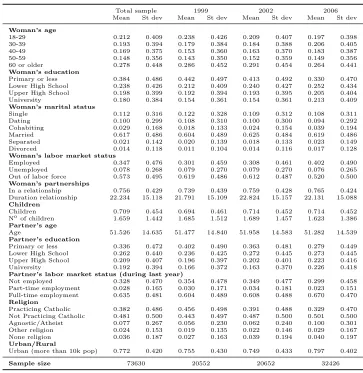
The sample for the analysis of the impact of divorce law on non-extreme abuse consists of the waves of 1999, 2002, and 2006 of the Survey of Violence Against Women. Table 1.1 presents the main descriptives statistics of the data. The number of observations is 20.552 in 1999, 20.652 in 2002, and 32.426 in 2006. Important for the validity of the difference-in-differences approach with repeated cross-sectional data is that samples come from the same population. This seems to be the case when we observe the sample composition in terms of the main observed characteristics (Table 1.1).

It is interesting to see how the different measures of intimate partner abuse relate to each other. As expected, all correlation coefficients are positive and statistically significant. The coefficient for the correlation between self-reported and technical abuse is 0.326. Moreover, according to the correlation between self-reported abuse and the four types of violence in which technical abuse can be decomposed, it is possible to deduce that women who declare to be victims of abuse tend to associate this situa-tion to physical abuse (ρ= 0.464), more than to psychological (emotional) abuse (ρ = 0.374), psychological abuse in the form of control (ρ = 0.322), or sexual abuse (ρ= 0.153).

(51)

insuf-ficient to convincingly prove the validity of the common trend assumption, the evidence available points in that direction.

Extreme Violence: Female Homicide

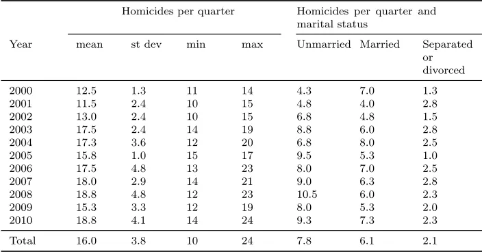
The sample for the analysis of extreme violence includes all 703 female homicides committed by intimate partners between 2000 and 2010 in Spain. During this period, the average number of female homicides per quarter is 16, with a minimum of 10 and a maximum of 24 (Table 1.2). In terms of the female population in Spain between 2000 and 2010, this translates into a quarterly prevalence of 0.88 female homicides per million women, or equivalently, 3.5 female homicides per million women and year.

According to the victim-offender relationship, in a typical quarter between 2000 and 2010, were killed in Spain 7.8 unmarried women, 6.1 married women, and 2.1 separated women.45

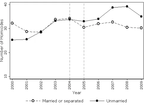
Figure 1.7 provides some evidence in favor of the common trends assump-tion for the difference-in-differences approach employed here. It shows the evolution of the number of intimate partner female homicides by marital group for the period between 2000 and 2010. Both the level and the year-to-year variation of the number of homicides are relatively similar for both treatment and control group, particularly in the years close to the legal change (2002-2004).

45_{As mentioned in Section 1.4, it is not possible to distinguish between separated and}

(52)

1.5 Empirical Results

a Non-Extreme Violence

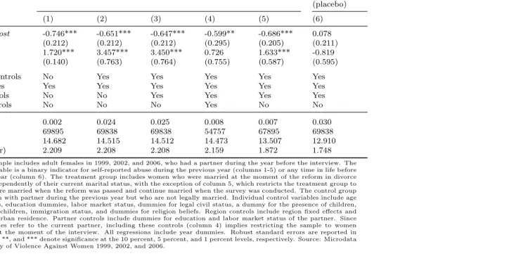
Table 1.3 shows the results of equation 1.4 when the dependent variable is the dummy for self-reported abuse. Column 1 presents the results for a specification with no controls beyond the treatment indicator and year dummies. The difference-in-differences coefficient suggests a decline in self-reported abuse for the treatment group in comparison with the control group after the reform in divorce law by 0.75 percentage points. In column 2, I add individual-level controls -age, education, labor market status, le-gal civil status, presence and number of children, immigration status, and religion beliefs, while in column 3 I also include region fixed effects and a dummy for urban residence. After controlling for individual characteristics and aggregated variables, the estimated coefficient remains negative and statistically significant. In the preferred specification (column 3), easier di-vorce reduces self-reported abuse by 0.65 percentage points (29 percent of the sample mean). If we want to control for partner’s education and labor market status, we need to restrict the sample to women with a partner at the moment of the interview.46 This is reported in column 4, which shows that self-reported abuse decreases by 0.59 percentage points (27 percent of the sample average).

The estimate reported in column 3 reflects the impact of easier divorce on domestic violence through the two possible channels: the dissolution of abusive marriages and the decrease in violence among intact households. In order to capture the change in domestic violence explained by a change in wife’s bargaining position within the household, column 6 reports the results when the treatment group is restricted to women who were already married when the law was passed and continued married at the moment of the survey. The coefficient not only remains negative and precisely

es-46_{While self-reported abuse refers to previous year, partner’s information is only}