Network externalities across financial institutions
Carlos Castro
Juan S. Ordoñez
Sergio Preciado
SERIE DOCUMENTOS DE TRABAJO
No. 184
Network externalities across financial institutions
Carlos Castro, Juan S. Ordo˜
nez, Sergio Preciado
∗Facultad de Econom´ıa, Universidad del Rosario, Colombia
February 28, 2016
Abstract
We propose and estimate a financial distress model that explicitly accounts for the interactions or spill-over effects between financial insti-tutions, through the use of a spatial continuity matrix that is build from financial network data of interbank transactions. Such setup of the finan-cial distress model allows for the empirical validation of the importance of network externalities in determining financial distress, in addition to institution specific and macroeconomic covariates. The relevance of such specification is that it incorporates simultaneously micro-prudential fac-tors (Basel 2) as well as macro-prudential and systemic facfac-tors (Basel 3) as determinants of financial distress. Results indicate network externalities are an important determinant of financial health of a financial institutions. The parameter that measures the effect of network externalities is both economically and statistical significant and its inclusion as a risk factor reduces the importance of the firm specific variables such as the size or degree of leverage of the financial institution. In addition we analyse the policy implications of the network factor model for capital requirements and deposit insurance pricing.
Keywords: systemic risk; network models; spatial econometrics. JEL Classification: C21,C58,G32.
1
Introduction
The 2007-2008 financial crisis has shifted the focus from the assessment of the resilience of individual financial institutions towards a more systemic approach. Hence, macro-prudential supervision and regulation will play a vital role in the new financial architecture, on Banking Supervision (2010). The crisis vividly showed the complex interconnections within the financial system, in particular how problems in some institutions could easily be transmitted to other institu-tions independently of how far from each other they appeared to be. Although, in the last thirty years we have witnessed important efforts toward the standard-ization of financial regulation and supervision around the globe (Basel 1), as well
as the implementation of techniques that made financial institutions more aware of the risk they were facing in their own portfolios (Basel 2), systemic risk was largely overlooked. Basel 2 placed a strong emphasis on how each financial in-stitution was able to integrate their credit and market information, in a timely manner, so as to determine and quantify the level of risk of the portfolio and calibrate the required capital. In general there was a myopic focuss on the micro-prudential side of financial supervision. Financial literature also gave a strong role to the firm specific level determinants (firm size and age, financial ratios, among others) of financial distress along with a set of macroeconomic cyclical components (Ergungor and Thomson (2005); Laeven and Majnoni (2003); Uhde and Heimeshoff (2009)). To a great extent this myopic view has changed due to the financial crisis. Basel 3 strongly advocates financial regulation focused on limiting systemic risk among other issues like defining a liquidity ratio standard and controlling for excessive leverage. The magnitude of systemic risk and the consequences of accumulating such risk, mostly depends on the collective behav-ior of the financial institutions, their interconnections (within the system) and their connections to the rest of the economy. The mapping of such connections is fast becoming an important tool for macro-prudential supervision.
After the Great Depression, policymakers were faced with the daunting task of rethinking the way economic activity was measured. These innovations lead to the development of comprehensive set of national income accounts. Brun-nermeier et al. (2011), argue that we now face a similar task, because during 2007-2008 financial crisis policymakers found themselves without the relevant information about the linkages within the financial sector as well as the linkages to the real economy.
The challenge of building this risk topography has received important method-ological feedback from network and graph theory. This branch of mathematics has provided a set of definitions, tools, techniques that have been extensively applied to analyze financial networks, Newman (2010). Financial network mod-els have been developed both at the theoretical level as well as the empirical or applied level. Theoretical models have focused on identifying how a partic-ular topology of the financial system can channel and amplify shocks affecting a single financial institution. In other words the question has been: How does a particular structure (topological structure) of the financial system provides higher or lower systemic risk and resilliance? Various simple models (Allen and Gale (2000), Babus (2005), Glasserman and Young (2015), Haldane (2009)) have addressed the robust-yet-frigile property of the financial system. This property illustrates a trade-off with respect to the number of interconnections within the system, because connections serve both as shock-absorbers as well as shock-amplifiers. One of the main results and more or less a consensus that has emerged is that, when the network is not too much connected; then the higher the connectivity of the system, the higher risk-sharing and diversifica-tion. However, above a certain connectivity threshold, those connections that before served as mutual insurance against shocks, can now act as factors that aggravate an initial adverse shock to the system.
us-ing data on financial counterparts across and within countries to map existus-ing networks, and in some cases analyze the robustness of financial systems using simulations (see Anand et al. (2009); Boss et al. (2003); Castr´en and Kavo-nius (2009); Bastos and Cont (2010); Cajueiro and Tabak (2007); Degryse and Nguyen (2007); Chan-Lau (2010a,b); Espinosa-Vega and Sole (2010)). Most of these applications use either simple reaction functions based on balance sheet identities or more complex agent-base models, that interact with the observed network maps and through a series of simulations generate different types of indicators of financial stability.
Within the financial network literature there is an emerging literature that use network data and econometric techniques (Jorion and Zhang (2009); Signori and Gencay (2012); Keiler and Eder (2013)). There is a well consolidated literature in social interaction models: Manski (1993); Durlauf and Young (2001), and their respective empirical applications in education Lin (2005), and technology adoption(Case (1992), just to name a few. More recently, the links to these social interaction model and the spatial autoregressive model (SAR) in the spa-tial econometric literature has been well established, Lee (2007, 2004). Beyond financial networks there is an active field of research on the econometrics of network data (see de Paula (2015) for a complete survey). Econometric models related to network data for the moment have the following intentions: a) models where a particular outcome of interest are mediated by predetermined networks (a prime example of this is social interaction models); b) models for network formation and with a possibility of analysing the joint determination of both network formation and outcomes mediated by these evolving networks; or c) measurement issues related to networks and outcomes.
In this paper we introduce the interconnections between financial institu-tions, through the use of a spatial continuity matrix, as predictor of financial distress. The introduction of the interconnections allows us to determine the importance of network externalities after controlling for firm specific effects as well as macroeconomic factors. These network externalities will allow us to de-termine how fragile are the institutions to the complex interconnections that may lay hidden with in the financial system. From a methodological point of view we are interested in how a given observed network determines how fragile is a particular financial institution, that is we are interested on how the exist-ing network configuration has an effect on an outcome variable such a fragility. We estimate the financial distress model using a panel of financial institutions from the colombian financial sector. In addition we explore how such models could potentially be used in a particular policy setting such as the definition of capital requirements or the premiums paid for deposit insurance by financial institutions. Our interest is to introduce a discussion on the use of econometric network models to quantify fragility and potentially illustrate the challenges.
supplier-customer network across firms. Their results indicate that network effects, measured as the leverage of its main customers, are as important as the firms own leverage in its effect over the credit spread. In a recent paper Keiler and Eder (2013) using a methodological approach similar to ours, propose a spatial autoregressive model to estimate a three factor model on CDS spreads for 15 financial institutions in Germany. One of the factors captures the interrelation or distance between the financial institutions. The distance across financial in-stitutions are approximated using a standardized correlation matrix based on the stock market information for the financial institutions.
The results indicate that network externalities are an important factor to de-termine financial health of an institution. Under different sets of specifications and control variables we find that the financial health of institutions that are interconnected has a positive (economically and statistically significant) feed-back effect on the financial health of the institution in question. The result are in line with the macroprudential approach of basel 3 as a complementary tool to microprudential supervision advocated in basel 2. Our framework, the network factor model, provides a way to: a) links macroprudential supervision to standard microprudential factor models, and b) provides a first approach to measure financial fragility across financial institutions.
We provide a discussion on the the policy implications of the results. Al-though the notion and measurement of systemic risk, contagion or network externalities for that matter has always been a relevant issue for regulators and academics, there is still no concrete and well accepted methodology to incor-porate the relevance of these interconnections in a concrete capital requirement formula or in terms of deposit insurance pricing. We survey the exiting literature and find some approaches to introduce interactions across financial institutions, however, there are still many unsolved issued regarding how to do so with capital requirement or deposit insurance pricing principles, and the empirical evidence with regard to the importance of interconnections.
The remainder of the paper is organized as follows. Section 2 presents the fi-nancial network information that we will use to quantify the interconnections across the institutions. In section 3 we introduce a network factor model for credit risk. Section 4 provides a brief discussion of the empirical results. Sec-tion 5 discusses the literature on capital requirements and interconnecSec-tions and deposit insurance pricing. Section 6 concludes.
2
Financial network data and spatial continuity
Definition
A network (graph) G consist of a non-empty set of elements V called vertices, and a list of unordered pairs of these elements called edges E. The set of vertices (nodes) of the network is called a vertex set and the list of edges is called edge list.
An edge is identified by an ordered pair of vertices. In other words, if i and j are vertices of G, then an edge of the form (i,j) is said to joint or connect i and j.
The functions G can take many forms, although the most common are as follows:
G:V XV → {0,1} (1)
such that G(i, j) = 1 if and only if there is an edge between (i, j). In most cases there are no self loops such that G(i, i) = 0 ∀i. This particular form of the functionGonly considers the existence of a link between the edges without taking into account the possible strength of such relationships. Another possible interpretation for the function is that of a distance function between verticesi
andj, Pinksey and Slade (2009), different to the binary measure (1).
G:V XV →R (2)
such thatG(i, j) determines the strength of the relationship between institutions
iandj. In both cases the functionGcan be interpreted as a square (adjacency) matrixW, where G(i, j) =wi,j. Such adjacency matrix is row normalized by
dividing each element by the sum of it entries, ˜wi,j=∑ V j=1wi,j.
The financial network we use is build from the information of a large value payment system administered by the Central Bank of Colombia (Banco de la Republica). The vertices represent the financial institutions and the edges rep-resent (in COP) the value of the transactions that are registered in the payment system. Element wi,j corresponds to the payment from institution i to
insti-tutionj. Each element was expressed as a percentage of the total value of the transaction during the time frame when the transactions are recorded.
3
Network factor model
Most models of financial distress derived their specification from structural credit risk literature (Merton type models). The model we propose incorpo-rates the standard the elements of a financial distress model: a)yi,t a proxy for
the financial health of institutioni at timet, b) a set of institution specific co-variatesXi,t, c) a set r macroeconomic covariatesZt, and d) possible some firm
specific non-observable effects. The fundamental difference is the introduction of the spatial continuity matrixW. In the section 2 we have shown how we can use the information from a financial network model to build a spatial continuity matrix that quantifies the interconnections across the institutions.
whereW yi,t is a standardized measure of the distance to some possible troubled
institutions andεi,t∼(0, σ2). The distance is measured using the observed
in-terbank interactions across the institutions determined by the financial network data. Thereforeρwill indicate the relative importance of the average distress of institutions close (where the measure of closeness is established according to the level of interbank transactions) to institutionsi.
From the supervisors point of view the set of determinants of financial health for a financial institution can be organized into two groups: first, the risk factor factors advocated by the microprudential aspects of Basel 2. Such as firm spe-cific variablesXi,tand state variables (primarily macroeconomic conditions)Zt.
Second, the risk factors advocated by the macroprudential outlook of Basel 3. Mainly, the importance of the interconnections across the financial institutions.
y= ρWy
| {z }
Basel III
+αι+βX+γZ
| {z }
Basel II
+ε (4)
As mentioned previouslyρmeasures the importance of network externalities as a determinant of financial distress, therefore this is our parameter of interest.
From an econometric point of view the financial distress models outlined above are nothing different than spatial autoregressive models (SAR) proposed by Cliff and Ord (1973).
y=ρWy+αι+βX+γZ+ε (5)
whereε∼(0, σ2
In). Anselin (1988); Anselin et al. (2008); Baltagi et al. (2003,
2007); Elhorst (2003); Kapoor et al. (2007); Yu et al. (2008) have extended the use of these method in a panel data setting. Estimation of these models is via maximum likelihood (where the distribution of the error is assumed to be Gaussian) or generalized method of moments (more precisely instrumental vari-ables). As a special case of GMM is an estimation strategy based on two-stage least squares with instrumental variables. Kelejian and Prucha (1998) shows that the estimators from this method are asymptotically efficient as long as the instruments are not correlated with the dependent variable. In the first stage we estimate the average distress of those institutions that have strong ties to finan-cial institution i(expression 3), where (ji,t) = (θ1xi,t, θ2W1xi,t, θ3W1). In the
second stage we use the estimated instrumentW\1yi,t to obtain the parameters
of interest (α, ρ, β, γ).
W1yi,t=θ(ji,t) +ui,t
yi,t=αi+ρW1y\i,t+βXi,t+γZt+εi,t
4
Empirical results
The introduction of the interconnections allows us to determine the impor-tance of network externalities after controlling for firm specific effects as well as macroeconomic factors. These network externalities will allow us to determine how fragile are the institutions to the complex interconnections that may lay hidden with in the financial system. We estimate the financial distress model using a panel of financial institutions from the colombian financial sector. We give a brief description of the financial network data. According to Leon (2013) the literature on financial networks recognizes two main data sources: financial transactions or balance sheet exposures. Financial transaction data is preferred to the later because it is highly detailed since it contains information on the origin and destiny of the transaction, the quantity, the type of transaction, the underlying assets involved, among other things. In addition it can be available in real time if you can monitor the register of transactions. On the other hand balances sheet financial exposures relies on the quality of accounting data and is subject to the strict oversight needs of the regulator, as such it is not provided on timely manner or the cross exposures between institutions might be difficult to identify.
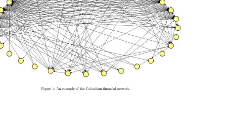
The contiguity matrix that we use for our estimation was constructed from the transaction level data registered in a high value payment system that is adminis-tered by the Central Bank of Colombia. The transactions represent the average conditions for the year 2009. The network, on which the contiguity matrixW
is based, is represented in figure 1 . Each interconection or {i, j} pair in the matrix corresponds to a payment form institutionito institutionj, expressed as a percentaje of the total transactions over the period of analysis for institution
i.
Although in the previous section we define the dependent variableyi,tas an
indicator of the fragility of institutioniat timet, in the empirical application we takeyi,tas the financial health of institutioni. There are different variables
point in time, these indicators are not available for financial institution that are not internationally active or in particular, for our data set are not available for all of the financial institutions that make up our representative sample of the Colombian Financial system. Some authors (Gorton (1990); Flannery and Sorescu (1996)) have tried to substitute the market information for the book value of the firm (in their financial statements), however they still require to make strong assumptions on the volatility of the value of the assets, which ends up driving the results. Because of the unavailability of market data on most financial institutions in Colombia (less than 25% of financial institutions have gone public) we resort to building a balance sheet based indicator on financial health.
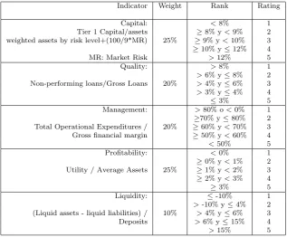
We apply the methodology known as CAMEL (Capital, Assets, Manage-ment, Earnings and Liquidity) to build a synthetic indicator of financial health. The CAMEL measure basically is a weighted average of financial balance sheet ratios. In particular, we use the CAMEL weights that the deposit insurance institution of Colombia (FOGAFIN) uses for pricing deposit insurance.
Table 1 presents the weights and balance sheet ratio that we have used to build the dependent variableyi,t, our proxy of financial health of each
in-stitution. Each of the financial ratios in table 1, is build with the monthly information (for the year 2009) reported by the financial institution supervisor (Superintendencia Financiera de Colombia).
The control variables that are included in the model characterize by expres-sion 3, include a set of firm specific variablesXi,t and macroeconomic variables Zt. The firm specific variables are:
• Leverage: for some time is has been known that highly levered financial institution are more prone to bankruptcy (Merton (1974); Crosbie and Bohn (2003)). The recent financial crisis showed that the most levered institutions were the most fragile and in grater risk of default.
• Size: larger institutions can be better equipped to handle changes in the economic environment or could simply be consider ex-ante too-big to fail. Keiler and Eder (2013) finds evidence that on average larger institutions have lower probabilities of default.
• Indicator variable that identifies whether a financial institution is domestic or foreign owned.
• Indicator variable that identifies if a domestic financial institution belongs to a financial conglomerate or group.
One of the limitations of using a CAMEL base indicator (as oppose to market based indicators like CDS spreads) for financial health is that we cannot intro-duce other firm specific balance sheet based control because they have a close relationship with the variables that are incorporated in the CAMEL measure.
(2009)). We are mainly interested in variables related to GDP (but with monthly frequency), inflation and real interest rates:
• Energy demand.
• 12 month inflation rate.
• average real interest rate.
• lagged unemployment rate.
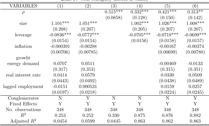
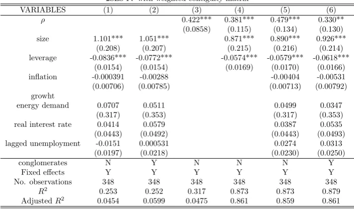
Tables 2 and 3 present the estimation results of expression 3. The difference between the tables is that in the former we use a matrixW obtained from a graph that only considers the existence of a link between the institutions (a matrix of ones and zeros before row standardization); while the later the same matrix is obtained from a graph that considers not only the existence of a trans-action between institution but also the magnitude of the transtrans-action. In other words in table 3 the spatial weights that are represented in W reflect a per-centage of the total value of the transaction during the time frame when the transactions are recorded. In both tables the first two columns do not take into account the network effects, only the fixed effects, the firm level variables and the macroeconomic controls. Columns three, four and five sequentially include the network effects with the firm level variables and the macroeconomic con-trols. Finally column six includes all of the previous variables plus the dummy variables for banking groups. All of the estimation presented include fixed effect for each financial institutions.
The first two columns in both tables represent the Basel 2 specification in expression 4, in the sense that financial health is only determined by firm specific variables and macroeconomic conditions. Both the size and leverage variables are significant and have the expected sign; larger institutions are healthier and more levered institutions have lower health scores. On the other, hand macroe-conomic conditions are not individually significant (they are jointly significant as indicated by joint significance test). The most likely reason for this last result is that the sample only considers one year of data therefore the sample length is not capturing medium term variation in the economic cycle. Column 2 also includes a dummy variable control for the existence of large financial groups in the Colombian financial sector, there is however no particular change in the estimated variables after controlling for this type of capital ownership. Further-more, we find that financial institution belonging to one of the large groups are not on average healthier than those that are not a part of a larger group.
average financial health score of its interconnected institutions; where the av-erage is determine by the existence of such interconnections or the strengths of the interconnections (measures in terms of the value of transactions).
5
Policy implications of network externatilies for
financial institutions
One of the most important concerns regarding the regulatory overhaul that came after the financial crisis was the measurement of systemic risk and how to account for such risk in terms of regulatory capital. Although, how do we measure systemic risk? is still an open question there seems to be a strong con-sensus regarding the importance of visible or hidden interconnections between the financial institutions, as a determinant of the extent of the crisis, in terms of the number of institutions affected and the ripple effects on the real economy1
. With this in mind, the most relevant question in terms of policy recommenda-tions, that can come out of specifying and estimating a network factor model is: how do we account for the relevance of interconnections between institutions for capital requirements (credit risk portfolio models) and deposit insurance pric-ing2
.
Most of the literature concerning default risk models augmented to account for interactions between firms, counterparty risk or contagion, follow the usual dis-tinction in the credit risk literature of structural (Egloff et al. (2007), Neu and Kunh (2004), Hatchett and Kuhn (2006)) or reduced form models (Giesecke and Weber (2004), Giesecke and Baeho (2011)). Our purpose is to establish an analogy between portfolio credit risk models for determining capital require-ments and a similar problem for financial regulators in managing the financial health of individual institutions that make up the financial system. In standard portfolio credit risk models the purpose is to estimate economic capital and al-locate these requirements to the different positions of the portfolio. In a similar vein financial regulators are interested in the possibility that the financial health of each financial institution is not only affected by its own characteristics but also by the financial health of the institutions that are very connected to the institution of interest.
The workhorse of portfolio credit risk models is the so-called Asymptotic risk factor model (Aas (2005), De Servigny and Renault (2004)). In this model changes in the creditworthiness of the positions in the portfolio are driven by a systematic and an idiosyncratic factor. As every position in the portfolio
1
The open question is in fact broader because some proposals to measure systemic risk can actually be measuring the fragility of a financial institution to shocks in other institutions rather than the effect of a particular large or very connected institution on the system as a whole.
2
becomes in relative terms less important (more and more fine-grained) idiosyn-cratic risk is diversified away. In this context, and more general in the Basel II framework, one can show that the portfolio wide capital charge is the sum of the individual capital charges for every position (asymptotic capital additivity). In this framework capital per dollar of exposureCτ(L), at some confidence level τ, depends primarily on the difference between unexpected losses (qτ(L)) and
expected losses (E(L)) from the portfolio.3
.
Cτ(L) =qτ(L)−E(L) (6)
qτ(L) = N
∑
i=1
wisiP(yi<Φ− 1
(pi)) (7)
P(yi<Φ− 1
(pi)) = Φ(
Φ−1(pi) +√ρiΦ−1(α)
√
1−ρi
) (8)
E(L) =
N
∑
i=1
wisipi (9)
where wi is the weight of exposure i, pi is the probability of default, P(yi <
Φ−1(pi)) is the conditional (on the systematic factor) probability of default,si
is the loss given default andρi is the average asset correlation of positioniwith
the other elements in the portfolio.
As we mentioned previously we make an analogy with the problem of the reg-ulator and consider i as an institution, as a position in the portfolio of the regulator. In the context of conterparty credit risk Neu and Kunh (2004) pro-poses an expression for the conditional probability of default 8 that takes into account the interconnections between a network of firms. Following Neu and Kunh (2004) we formulate a conditional probability of default for a financial institution. The difference is that the conditioning variables are the factors in the network factor model 3.
From section 3 yi,t denotes a variable that proxies the financial health of
fi-nancial institution i at time t. As in any structural credit risk model if yi,t
falls below a threshold then the financial institution goes into bankruptcy. Now for simplicity suppose this threshold is an unobserved institution specific factor
αi+ Φ−1(pi) then from expressions 8 and 3 we have,
P(yi<Φ− 1
(pi)) = Φ(
Φ−1(pi) +ρ\W yi,t+βXi,t+γZt
σ ) (10)
In order to satisfy the distributional assumptions we must impose some re-strictions on the loading coefficients of the factors as well asσ. σis usually a function of the loading coefficients of the factor. We do not derive an explicitly formulas imposing some restrictions, however Egloff et al. (2007) derives a re-cursive numerical method to derive such representation for a similar model that
3
accounts for credit contagion using a spatial contiguity matrix that is called the business matrix because it (i, j)−elements indicate the strengths of the business interdependence between counterparties in a network. With this conditional probability of default based on the network factor model we can in theory use the empirical model presented in the previous section to obtain a capital charge. This capital charge will be sensible not only to the specific characteristics of the financial institution and the macroeconomic conditions but will also incorpo-rate the conditions of the institutions that are connected to the institution of interest. However, this capital charge is more related to the concept of fragility rather than systemic importance, Castro and Ferrari (2010). Therefore, such capital charge should probably not be levied on systemically important financial institutions (SIFI’s) but rather the institutions that are at the periphery of the network.
The idea of measuring the fragility of a financial institution could actually make much more sense, not only methodologically but also from the point of view of the regulator and supervisor, in terms of deposit insurance pricing rather a formal capital charge. The main reason is that institutions that are heavily reliant on liquidity provision from the central players in the financial network will also be the institutions that are more fragile during period of widespread bank failure. Hence in the aftermath of their own failure the recovery value on their assets will be probably much lower than for the other institutions in the network (Acharya and Yorulmazer (2010))4
. Ex-ante the actuarially fair deposit insurance premium for more fragile institutions should be larger. If this were the case the network factor model could play the role of accounting for the sensibility of interconnections in the deposit insurance premium. In par-ticular, deposit insurance pricing at many deposit insurance institutions is a function of a proxy of the financial health of the institution such as CAMELS ratings Bloecher et al. (2003). The network factor model and our empirical re-sults provides a risk mapping that includes network externalities, therefore for a given deposit insurance pricing scheme mapped to such CAMELS ratings it would be feasible from our result to account for interconnections across financial institutions.
6
Conclusions
The empirical results from the network factor model indicate the importance of network externalities, quantified through the strength of interconnections be-tween financial institutions. The spatial econometric model provides an statisti-cal methodology that is in line with recent efforts to include network information to explain outcomes of interest, in this case the health or creditworthiness of a financial institution. With this model we are able to confirm that the average
4
financial health of those institutions for whom the institutions of interest shares a sizable relationship have an important and a significant effect on the financial health of an institution of interest. Our results are based on a set of Colombian financial institutions: their balance sheet information, the transactions, and fi-nancial health indicators used for deposit insurance pricing.
With the empirical results at hand we survey the literature an discuss the im-pact of network factor models on the quantification of capital requirements and deposit insurance premiums. We conclude that the network factor model can be used for capital requirements, however such requirements should be levied on the most fragile institutions in the network, that is those institutions whose financial health are heavily affected by the situation of the other (connected) institutions. Therefore, our capital requirement measure is not intended for systemically important institutions (SIFI’s). Following a similar argument the network factor model can also be a tool for pricing deposits insurance under the premise that the expected cost to the deposit insurance provider should not only increase in relation to individual bank failure but also in relation to joint bank failure risk.
Acknowledgements
References
Aas, K. (2005). The basel ii irb approach for credit portfolios: A
survey. Technical report, Norwegian Computing Center.
Acharya, V. V.and Santos, J. and Yorulmazer, T. (2010). Systemic
risk and deposit insurance premiums.
FRBNY Economic Policy
Review
, pages 89–100.
Allen, F. and Gale, D. (2000). Financial contagion.
Journal of
Political Economy
, 108:1–33.
Altman, E. I. (1968). Financial ratios, discriminant analysis and
the prediction of corporate bankruptcy.
The journal of finance
,
23(4):589–609.
Anand, K., Brennan, S., Kapadia, S., Willison, M., and Gai, P.
(2009). Complexity and crises in financial systems.
Anselin, L. (1988).
Spatial econometrics: methods and models
,
vol-ume 4. Springer.
Anselin, L., Le Gallo, J., and Jayet, H. (2008).
Spatial panel
econometrics. In
The econometrics of panel data
, pages 625–660.
Springer.
Babus, A. (2005).
Financial Development, Integration and Stability
,
chapter Contagion risk in financial networks, pages 423–440. UK:
Edward Elgar.
Baltagi, B. H., Egger, P., and Pfaffermayr, M. (2007). A generalized
spatial panel data model with random effects. Technical report,
Working Paper, Syracuse University.
Baltagi, B. H., Song, S. H., and Koh, W. (2003). Testing panel
data regression models with spatial error correlation.
Journal of
econometrics
, 117(1):123–150.
Bastos, E. and Cont, R. (2010). The brazilian interbank network
structure and systemic risk.
Bloecher, E., Seale, G., and Vilim, R. (2003). Options for pricing
Boss, M., Elsinger, H., Summer, M., and Thurner, S. (2003). The
network topology of the interbank market.
Brunnermeier, M. K., Gorton, G., and Krishnamurthy, A. (2011).
Risk topography.
NBER Macroeconomics Annual
, 26(1):149–176.
Cajueiro, D. O. and Tabak, B. M. (2007). The role of banks in the
brazilian interbank market : Does type bank matter?
Case, A. (1992). Neighbourhood influence and technological change.
Regional science and urban economics
, 22:491–508.
Castr´en, O. and Kavonius, I. K. (2009). Balance sheet interlinkages
and macro-financial risk analysis in the euro area.
Castro, C. and Ferrari, S. (2010). Measuring the systemic
impor-tance of financial institutions using market information. Technical
report, Financial stability review National Bank of Belgium.
Chan-Lau, J. A. (2010a). Balance sheet network analysis of
too-connected-to-fail risk in global and domestic banking systems.
IMF Working Papers.
Chan-Lau, J. A. (2010b).
Regulatory capital charges for
too-connected-to-fail institutions: A practical proposal. IMF Working
Papers.
Cliff, A. D. and Ord, J. K. (1973).
Spatial autocorrelation
. London
Pion.
Crosbie, P. and Bohn, J. (2003). Modeling default risk.
de Paula, A. (2015). Econometrics of network models.
De Servigny, A. and Renault, O. (2004).
Measuring and managing
credit risk
. McGrawHill.
Degryse, H. and Nguyen, G. (2007). Interbank exposures: An
empir-ical examination of contagion risk in the belgian banking system.
International Journal of Central Banking
.
Durlauf, S. and Young, H. (2001).
Social Dynamics
, chapter The
new social economics, pages 1–14. MIT: Press.
Egloff, D., Leippold, M., and Vanini, P. (2007). A simple model of
Elhorst, J. P. (2003). Specification and estimation of spatial panel
data models.
International regional science review
, 26(3):244–268.
Ergungor, O. E. and Thomson, J. B. (2005). Systemic banking
crises.
Policy Discussion Papers
, (Feb).
Espinosa-Vega, M. A. and Sole, J. (2010). Cross-border financial
surveillance: A network perspective.
Flannery, M. J. and Sorescu, S. (1996). Evidence of bank market
dis-cipline in subordinated debenture yields: 19831991.
The Journal
of Finance
, 51(4):1347–1377.
Giesecke, K. and Baeho, K. (2011). Systemic risk: What defaults
are telling us.
Management Science
, 57(8):1387–1405.
Giesecke, K. and Weber, S. (2004). Cyclical correlations, credit
contagion and portfolio losses.
Journal of Banking and Finance
,
28:3009–3036.
Glasserman, P. and Young, H. P. (2015). How likely is contagion in
financial networks?
Journal of Banking & Finance
, 50:383–399.
Gorton, G.and Pennacchi, G. (1990). Financial intermediaries and
liquidity creation.
The Journal of Finance
, 45(1):49–71.
Haldane, A. G. (2009). Rethinking the financial network. In
Speech
delivered at the Financial Student Association
.
Hatchett, J. and Kuhn, R. (2006). Effects of economic interactions
on credit risk.
Journal of Physics A: Mathematical and General
,
39:2231–2251.
Jorion, P. and Zhang, G. (2009). Credit contagion from counterparty
risk.
The Journal of Finance
, LXIV:2053.
Kapoor, M., Kelejian, H. H., and Prucha, I. R. (2007). Panel data
models with spatially correlated error components.
Journal of
Econometrics
, 140(1):97–130.
Kelejian, H. and Prucha (1998). A generagener spatspa two-stage
least squares procedure for estimating a spatial autoregrautore
model with autoregrautore disturbances.
The Journal of Real
Es-tate Finance and Economics
, 17(1):99–121.
Laeven (2004). The political economy of deposit insurance.
Journal
of Financial Services Research
, 26(3):201–224.
Laeven, L. and Majnoni, G. (2003). Loan loss provisioning and
economic slowdowns: too much, too late?
Journal of Financial
Intermediation
, 12(2):178–197.
Lee, L. (2004). Asymptotic distributions of quasi-maximun
likeli-hood estimators for spatial econometric models.
Econometrica
,
72:1899–926.
Lee, L. (2007). Identification and estimation of econometric
mod-els with group interactions, contextual factors and fixed effects.
Journal of Econometrics
, 140:333–74.
Leon, C.and Berndsen, R. (2013). Modular scale-free architecture
of colombian financial networks: Evidence and challenges with
financial stability in view. Technical report, Banco de la Republica
de Colombia.
Lin, X. (2005). Peer effects and student academic achivement: an
application of spatial autoregressive model with group
unobserv-ables. Technical report, Ohio State University.
Manski, C. (1993). Identification of endogenous social effects: the
reflection problem.
Review of Economic Studies
, 60:531–42.
Merton, R. C. (1974). On the pricing of corporate debt: The risk
structure of interest rates*.
The Journal of Finance
, 29(2):449–
470.
Neu, P. and Kunh, R. (2004). Credit risk enhancement in a network
of interdependent firms.
Physica A
, 342:639–655.
Newman, M. (2010).
Networks: An Introduction
. Oxford University
Press.
Pinksey, J. and Slade, M. E. (2009). The future of spatial
econo-metrics. Technical report, The Pennsylvania State University.
Signori, D. and Gencay, R. (2012). Economic links and counterparty
risk. Technical report, Simon Fraser University.
Uhde, A. and Heimeshoff, U. (2009). Consolidation in banking and
financial stability in europe: Empirical evidence.
Journal of
Bank-ing & Finance
, 33(7):1299–1311.
Yu, J., de Jong, R., and Lee, L.-f. (2008). Quasi-maximum likelihood
estimators for spatial dynamic panel data with fixed effects when
both¡ i¿ n¡/i¿ and¡ i¿ t¡/i¿ are large.
Journal of Econometrics
,
Indicator Weight Rank Rating
Capital: <8% 1
Tier 1 Capital/assets ≥8% y<9% 2
weighted assets by risk level+(100/9*MR) 25% ≥9% y<10% 3
≥10% y≤12% 4
MR: Market Risk >12% 5
Quality: >8% 1
>6% y≤8% 2
Non-performing loans/Gross Loans 20% >4% y≤6% 3
>3% y≤4% 4
≤3% 5
Management: >80% o<0% 1
≥70% y≤80% 2
Total Operational Expenditures / 20% ≥60% y<70% 3
Gross financial margin ≥50% y<60% 4
<50% 5
Profitability: <0% 1
≥0% y<1% 2
Utility / Average Assets 25% ≥1% y<2% 3
≥2% y<3% 4
≥3% 5
Liquidity: ≤-10% 1
>-10% y≤4% 2
(Liquid assets - liquid liabilities) / 10% >4% y≤6% 3
Deposits >6% y≤15% 4
[image:20.595.147.465.123.385.2]>15% 5
2SLS-IV with contiguity matrix as binary
VARIABLES (1) (2) (3) (4) (5) (6)
ρ 0.515*** 0.332*** 0.421*** 0.313**
(0.0858) (0.128) (0.150) (0.142)
size 1.101*** 1.051*** 1.002*** 1.026*** 1.008***
(0.208) (0.207) (0.205) (0.207) (0.207)
leverage -0.0836*** -0.0772*** -0.0705*** -0.0718*** -0.0699***
(0.0154) (0.0154) (0.0156) (0.0158) (0.0157)
inflation -0.000391 -0.00288 -0.00167 -0.00374
(0.00706) (0.00785) (0.00699) (0.00780)
growht
energy demand 0.0707 0.0511 -0.00469 -0.0133
(0.317) (0.353) (0.315) (0.351)
real interest rate 0.0414 0.0579 0.0330 0.0509
(0.0443) (0.0492) (0.0438) (0.0489)
lagged employment -0.0151 0.000531 0.0159 0.0257
(0.0197) (0.0218) (0.0224) (0.0245)
Conglomerates N Y N N N Y
Fixed Effects Y Y Y Y Y Y
No. observations 348 348 348 348 348 348
R2
0.253 0.252 0.330 0.875 0.876 0.882
AdjustedR2
0.0454 0.0599 0.0445 0.863 0.862 0.863
[image:21.595.136.484.257.467.2]Standard errors in parenthesis *** p<0.01, ** p<0.05, * p<0.1
2SLS-IV with weighted contiguity matrix
VARIABLES (1) (2) (3) (4) (5) (6)
ρ 0.422*** 0.381*** 0.479*** 0.330**
(0.0858) (0.115) (0.134) (0.130)
size 1.101*** 1.051*** 0.871*** 0.890*** 0.926***
(0.208) (0.207) (0.215) (0.216) (0.214)
leverage -0.0836*** -0.0772*** -0.0574*** -0.0579*** -0.0618***
(0.0154) (0.0154) (0.0169) (0.0170) (0.0166)
inflation -0.000391 -0.00288 -0.00404 -0.00531
(0.00706) (0.00785) (0.00713) (0.00792)
growht
energy demand 0.0707 0.0511 0.0499 0.0347
(0.317) (0.353) (0.317) (0.353)
real interest rate 0.0414 0.0579 0.0387 0.0535
(0.0443) (0.0492) (0.0443) (0.0493)
lagged unemployment -0.0151 0.000531 0.0274 0.0313
(0.0197) (0.0218) (0.0230) (0.0250)
conglomerates N Y N N N Y
Fixed effects Y Y Y Y Y Y
No. observations 348 348 348 348 348 348
R2
0.253 0.252 0.317 0.873 0.873 0.879
AdjustedR2
0.0454 0.0599 0.0475 0.861 0.859 0.861
Standard errors in parenthesis *** p<0.01, ** p<0.05, * p<0.1
[image:22.595.136.493.257.467.2]