Comparative Analysis of AI Techniques to Correct the
Inconsistency in the Analytic Hierarchy Process Matrix
Fabián Favret1, Federico Matías Rodríguez1, Marianela Daianna Labat1 1 Department of Engineering and Production Sciences, Universidad Gastón Dachary,
Posadas, Misiones, Argentina,
{fabianfavret@, rfedericomatias@, daiannalabat@} gmail.com
Abstract. The Analytic Hierarchy Process (AHP) is one of the most used techniques for decision making. The complex properties of its structure allow considering the subjectivity in the judgment of the experts but also arising a considerable degree of inconsistency when the pairwise judgments of the alternatives are computed. This research paper makes a comparison between two artificial intelligence methods for diminishing the inconsistency in the AHP pairwise comparison matrixes, the Backpropagation Neural Network (BPN) and Support Vector Machines (SVM).
Keywords: AHP, Multicriteria decisión making systems, SVM, BPN.
1 Introduction
There are a variety of tools that help with de decision making process and that allow to choose an alternative between many, using a diverse of comparative criteria, points of view, features, etc. A method widely used is the Analytic Hierarchy Process (AHP), a powerful tool for valuating available alternatives and differs of the other techniques in that it allows to include all the relevant factors for the decision making process, whether they are measurable, quantifiable o related with the strengths of the preferences, feelings of subjectivities. The results can be classified and ranked, and it is possible to measure the level of consistency of the emitted judgments [1], i.e., if there are errors due to subjectivities arising from pairwise comparisons.
In pairwise comparisons some transitivity errors may arise, assigning erroneous importance values loaded with imprecision, uncertainty or incomplete data [2], causing inconsistencies that are complex to detect and fix when the matrix order is increased [3].
2 Analytic Hierarchy Process (AHP)
AHP is a method based in pairwise comparison that can be used to find the weights of the individual criteria or alternatives. Thomas L. Saaty developed it between the years 1971-1975. Saaty proposed a scale that can be used to measure the intensity between the pairwise comparisons in which each linguistic phrase is mapped to a value in a set of available values, represented by {9, 8, 7, 6, 5, 4, 3, 2, 1, 1/2, 1/3, 1/4, 1/5, 1/6, 1/7, 1/8, 1/9}. The value 9, for example, represents that the evidence favoring a feature over another is of the strongest possible, and the 1 means that both features contribute in the same manner to the objective. These matrices are square ( ) positive, reciprocal and can be defined as follows:
[
]
,
(1)where {9, 8, 7, 6, 5, 4, 3, 2, 1, 1/2, 1/3, 1/4, 1/5, 1/6, 1/7, 1/8, 1/9}, and = 1 when , . The element is a pairwise judgment between two features. According to this equation we have , i.e. for each element of the array exists a related reciprocal [7].
AHP allows for inconsistency because in making judgments people are more likely to be cardinally inconsistent than cardinally consistent because they cannot estimate precisely measurement values even from a known scale and worse when they deal with intangibles (a is preferred to b twice and b to c three times, but a is preferred to c
only five times) and ordinally intransitive (a is preferred to b and b to c but c is
preferred to a). To evaluate this consistency Saaty showed that the major eigenvector is the only plausible candidate to represent the priorities emerging from a near consistent positive reciprocal matrix [8].
The priority vector is the main eigenvector of the matrix; it is obtained by an iterative method called The Power Method that will be not described here. The previously mentioned matrix A can be perfectly consistent if the main eigenvalue is equal to . The Consistency Index (CI) is defined as follows:
, (2)
where is the matrix order. To calculate the Consistency Ratio (CR) the following formula must be used:
, (3)
where the Random Index (RI) is the average value of the CI for random matrixes (using the Saaty Scale), several authors have different RI depending on the method used in the simulations and the number of matrixes involved in the process. The RI table used in this paper is the one that Saaty determined by simulations in the Wharton School of the Universidad de Pennsylvania for matrixes of order 4, 5, 6, 7 and 8 [9].
less than 0.1 so that the matrix can be considered consistent, the smaller the CR is, the better is the matrix consistency [8].
3 Artificial Neural Network (ANN)
The ANN try to emulate the behavior of the biological neurons of the living beings. Briefly, we can establish that the main functional element of an ANN is a neural cell or neuron. The computational model defines the artificial neuron or automata as an element that possess an internal state, called activation level and receive signals that allows, in this case, change of state [10]. In this paper it is used an ANN of the multilayer perceptron, trained with an algorithm called back propagation.
3.1 Multilayer Perceptron (MLP)
The MLP is a generalization of the simple perceptron (created by Frank Rosenblatt in 1957) and arise as a consequence of the limitations of that architecture related to the problem of the nonlinear separability [10]. Several authors demonstrated that the MLP is a universal approximator, in the sense that any continuous function of a compact in can be approximated with and MLP with at least one hidden layer of neurons [11] [12], this places the model as a new class of functions for interpolation of nonlinear relations between input and output data. It has been chosen in this research for comparison because it has shown that positive optimization results can be obtained in the estimation of elements of the AHP pairwise comparison matrices [4] [5].
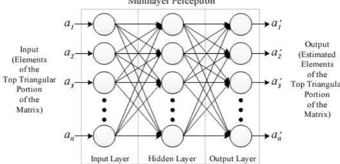
In MLP the neurons are grouped in three different layers, the input layer, the hidden layer and the output layer. The neurons in the input layer are responsible for receiving the signals or patterns from outside and propagate it to the neurons in the next layer. The last layer acts as an output and provides the network with a response to each of the input patterns.
As shown in the figure 1 the connections of the neurons in MLP are directed forward (that’s why it is called a feed forward network). The connections between the neurons are associated with a real number called weight, the weights of the hidden layer are denoted by , and thresholds , are the weights of the output layer, and his threshold [13]. Being the operation of an MLP represented by the following function:
∑ ∑ (∑ ) , (4) The activation function used in this research is the sigmoidal, which has as image a continuous range of values within the interval (0, 1), and is given by the following expression:
3.2 Backpropagation (BPN)
In the proposed method of ANN it is used a training rule denominated BPN. BPN is a mechanism of machine learning in which every parameter of the network is modified and adapted. In the MLP case is a supervised learning algorithm; i.e., the parameter modification is done so that the output of the network is as close as possible to the output provided by the supervisor or desired output. It is called back propagation because the error at the output of the network is propagated backwards becoming an error for each of the hidden neurons in the network [10].
3.3 Proposed Method of BPN
A neural network is built using three layers, the input layer has one neuron for each element of the input vector to be adapted to the different orders of the matrices which we work, these are 4×4, 5×5, 6×6, 7×7 y 8×8. The hidden layer has 80 neurons. In the training algorithm of BPN the learning rate (or alpha) is settled to 0.0001 and the momentum is 0.001. The epochs (or iterations) stop when the error is less than 0.01. Both the number of neurons of the hidden layer and the values of the learning rate and momentum has been chosen based on the experience and the behavior observed during the simulation runs. Each element of the pairwise comparison matrices is associated with a value between 1 and 17, for example: 1 equals to 1/9, 2 to 1/8 and so on, then these values are normalized between 0 and 1 in order to be used in the neural network with the sigmoidal activation function.
Fig. 1. Architecture of the proposed MLP method. The elements are the inputs and are the outputs of the network.
4 Support Vector Machines (SVM)
[image:4.595.126.463.428.591.2]Vladimir Vapnik in 1992 and subsequently optimized in 1995 along with Corinna Cortes in the laboratories of AT & T Bell [14]. In SVM to generalize, we want to choose such that is in some sense to the training examples. To this end a notion of similarity in (the domain) and {±1} (the outputs) is needed.
One of the advantages of the kernel methods is that learning algorithms developed are quite independent of the choice of similarity measure, allowing to adapt the latter to specific problems without the need to reformulate the learning algorithm [6].
4.1 Kernels as Similarity Measures
The role of the kernel then is to implicitly change the representation of the data into another (usually higher-dimensional) feature space. In SVM theory there are several kernels that can be used, in this research the Gaussian kernel has been chosen, its is also called Radial Basis Function (RBF) and can be expressed in the following manner:
‖ ‖ , with a suitable width . (8) RBF has two parameters, and ; they have diverse effects on the behavior of the SVM. Intuitively, the gamma parameter defines how far the influence of a single
training example reaches, with low values meaning ‘far’ and high values meaning ‘close’. The C parameter trades off misclassification of training examples against simplicity of the decision surface (a leads to an SVM of hard margin that allows over fitting). A low C makes the decision surface smooth, while a high C aims at classifying all training examples correctly.
4.3 Support Vector Regression
Instead of dealing with output of type , the estimation regression concerns in estimating functions with real value using . The estimation regression takes the form:
∑ , subject to (9)
where is zero for all the points that are inside the tube ε that is built by the model to enclose the data. Furthermore SVM regression uses a new loss function to calculate the error denominated of the form:
4.3 Proposed Method of SVM
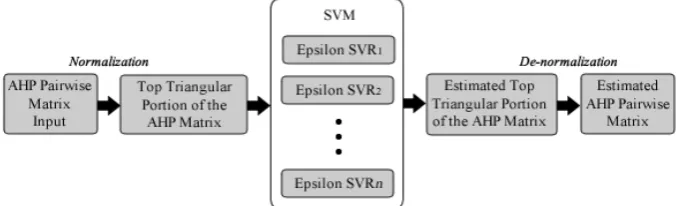
The proposed method in this research paper has the following SVM parameters: the SVM used is called Epsilon Support Vector Regression, because we need to make an estimate of real values. The kernel used is RBF. A SVM is trained for each element of the input vector, i.e. the number of SVM for regression will be (being the order of the AHP matrix). The parameters , of the SVM are chosen in a particular manner according to the behavior observed in the training used in this model, which is why they are applicable only to this domain according to the observations that were made. In the training, this method evaluates in each iteration a combination of and , in the SVM, if the error decrease then it goes to the next iteration, if not keeps trying all the possible combinations until all the possible values had been used; the range for = [1-100] and for = [1-100]. The iterations stop when the error is less than 0.01. In order to use SVM in a correct way the data must be previously normalized between 0 and 1.
Fig. 2. Architecture of the proposed method of multiple SVM for regression. Each
element of the input (1,2,…,n) is associated with an Epsilon SVR1, SVR2… SVRn
5 Description of the Simulations
5.1 AHP Pairwise Matrices
A total of 2000 matrices are taken in account for processing. These matrices are pairwise comparison matrices of the AHP that are normalized for the use in both machine learning methods, i.e., it is used only the superior triangular portion of each one because the main diagonal is always 1 and the inferior triangular portion of each matrix is the reciprocal of the superior. 1000 of those matrices are inconsistent; ergo they have a CR value of more than 0.1 and will be used as an input in the methods, while the other 1000 are consistent and will be used as ideals.
[image:6.595.127.466.335.438.2]5.2 Results Obtained
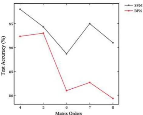
Based on the simulations we can highlight the superiority of SVM to BPN in terms of speed and number of iterations in the training of the model; during the testing phase it hast been observed in BPN a decrease of the precision when the order of the matrices are increased as shown in figure 3, however in SVM the percentage of successes remains homogeneous, except in the order 6, as shown in table 1.
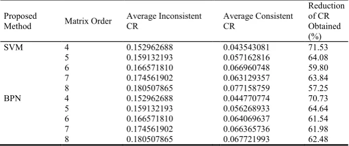
[image:7.595.124.475.353.481.2]In table 2, it is possible to see the average consistency ratio obtained from the output of the models in the test phase, and it is compared to the inconsistency of the original input elements, we can visualize that SVM has managed to play a positive role since the maximum percentage reduction achieved is 71.53% in contrast to BPN that has achieved 70.73%. BPN instead have a more uniform behavior in which the minimum reduction ratio reaches a 61.54% as contrasted with SVM that reached a minimum of 57.25%
Table 1. Summary of the results. The following table summarizes the results obtained using the two methods proposed for estimation.
Proposed Model Matrix Order Input Elements Iteration Number Training Time (sec.) Test Success Test Success Accuracy (%)
BPN 4 6 2957 6.60 277 92.33
5 10 474974 1293.36 279 93.00 6 15 1272121 4342.38 241 80.67 7 21 1573134 6609.38 248 82.67 8 28 1386544 7187.00 238 79.33
SVM 4 6 6 2.45 294 98.00
5 10 10 5.26 283 94.33
6 15 15 8.81 266 88.67
7 21 21 11.80 285 95.00
8 28 28 15.19 273 91.00
Table 2. Average CR values of inconsistence matrices and consistence ones of the test set.
Proposed
Method Matrix Order
Average Inconsistent CR Average Consistent CR Reduction of CR Obtained (%)
SVM 4 0.152962688 0.043543081 71.53
5 0.159132193 0.057162816 64.08 6 0.166571810 0.066960748 59.80 7 0.174561902 0.063129357 63.84 8 0.180507865 0.077158759 57.25
BPN 4 0.152962688 0.044770774 70.73
[image:7.595.121.475.517.665.2]Fig. 3. Accuracy obtained in the Tests, based in the matrices order, of each proposed method.
6 Conclusions
In this research two methods are implemented for correcting the inconsistency of the AHP pairwise comparison matrix, these methods are based on artificial intelligence tools, and are BPN and SVM. First, a BPN using a 3-layer MLP is implemented. Then a SVM for regression with a RBF kernel regression for each element of the input array is defined. Thirdly, simulations are performed, with training, validation and testing to be able to compare both methods. The SVM method has a behavior similar to BPN in CR reduction but with a better accuracy rate in predicting previously unknown inputs that are presented to the network and provides the advantage of a significantly faster convergence speed compared with the training speed of BPN.
Acknowledgments. To the collaborators who made this research possible.
7 References
1. Saaty, R.: The analytic hierarchy process—what it is and how it is used. In : Mathematical Modelling, Issues 3–5, vol. 9, pp.161–176 (1987)
[image:8.595.179.415.151.341.2]Structured tools and techniques. Pearson Education (2004) 1-11
4. Yi-Chung Hu, Jung-Fa Tsai: Backpropagation multi-layer perceptron for incomplete pairwise comparison matrices in analytic hierarchy process. In : Applied Mathematics and Computation, vol. 180, pp.53-62 (2006)
5. Gomez-Ruiz, J., Karanik, M., Peláez, J.: Estimation of missing judgments in AHP pairwise matrices using a neural network-based model. In : Applied Mathematics and Computation, vol. 216, pp.2959–2975 (2010)
6. Schölkopf, B., Smola, A.: Support Vector Machines. In : The Handbook of Brain Theory and Neural Networks. MIT Press, Cambridge, MA (2003) 1119-1125 7. Saaty, T.: How to make a decision: The Analytic Hierarchy Process. In :
European Journal of Operational Research, North-Holland, Nederlands, vol. 48, pp.9-26 (1990)
8. Saaty, T.: Decision-making with the AHP: Why is the principal eigenvector necessary. In : European Journal of Operational Research, Issue 1, vol. 145, pp.85–91 (2003)
9. Saaty, T.: The Analytic Hierarchy Process. McGraw-Hill, New York (1980) 10. Isasi Viñuela, P., Galván León, I.: Redes de Neuronas Artificiales. Un enfoque
práctico. Pearson Educación, Madrid, Spain (2004)
11. Hornik, K., Stinchcombe, M., White, H.: Multilayer feedforward networks are universal approximators. In : Neural Networks, vol. 2, pp.259-366 (1989)
12. Cybenko, G.: Approximation by superposition of a sigmoidal function. In : Mathematics of Control, Signals and Systems, vol. 2, pp.303-314 (1989)
13. Del Brío, M., Sanz, A.: Redes Neuronales Y Sistemas Borrosos. Alfaomega & Ra-Ma, Zaragoza, Spain (2007)
14. Vapnik, V., Cortes, C.: Support-Vector Networks. In : Machine Learning, New Jersey, vol. 20, pp.273-297 (1995)
15. Kecman, V.: Learning and soft computing. MIT Press, Cambridge, MA (2001) 16. Rychetsky, M.: Algorithms and Architectures for Machine Learning Based on