Hybridized Method
Leticia C. Cagnina and Susana C. Esquivel LIDIC (Research Group). Universidad Nacional de San Luis
Ej. de Los Andes 950 - (5700) San Luis, Argentina. {lcagnina,esquivel}@unsl.edu.ar
Abstract. This paper presents a hybrid method to solve hard multi-objective problems. The proposed approach adopts an epsilon-constraint method which uses a Particle Swarm Optimizer to get points near of the true Pareto front. In this approach, only few points will be generated and then, new intermediate points will be calculated using an interpola-tion method, to increase the among of points in the output Pareto front. The proposed approach is validated using two difficult multiobjective test problems and the results are compared with those obtained by a multiobjective evolutionary algorithm representative of the state of the art: NSGA-II.
1
Introduction
A great deal of problems that we find in science, industry and other areas, are a kind of a general optimization problem that involves multiple objectives. A multiobjective optimization problem (MOP) typically is formalized as the min-imization or maxmin-imization of [2]: f(x) = [f1(x), f2(x), . . . , fk(x)]T subject to
x∈X. In other words, we want a single solution xthat optimizes each one of thek different objective functions. The problem is that usually these functions forming a mathematical description of performance criteria, are in conflict with each other.
In MOP the quality ofxis no longer measures as a scalar (single objective op-timization case), but a vector with the values of the k objective functions. We might have that “x is better than y” which means that objective vector of x is better than that of the y in at least one objective, and no worse in all the others. This is named dominance and we say thatx dominates y. In the other hand, we might have a case in which “xis better thanyin some objectives, but yis better thanxin others”. This is namednon dominance and, we say thatx andy areincomparable or arenondominated.
The set of optimal solutions in X generally is denoted as Pareto set, and its image in the objective space as Pareto front. Therefore, the goal of the opti-mization is to find or approximate the Pareto set to obtain the Pareto front (the true) or some front close to it.
on the approximation of the Pareto set.
In the last years, some proposal for extending Particle Swarm Optimization (PSO) algorithms to treat MOPs, have been published [18, 6, 10, 9]. The Par-ticle Swarm strategy for optimization [5] uses a population of parPar-ticles to find solutions through hyperdimensional search space. The change of the particle’s position is based on the social-psychological tendency of individuals, to emulate the success of other individuals. Each particle has associated a velocity vector which drives the optimization process and reflects the socially exchanged infor-mation.
In this paper we propose an alternative algorithm to solve hard multiobjec-tive optimization problems, based on the mathematical programming technique named epsilon-constraint method, which was hybridized with a PSO algorithm to enhance the search process of solutions.
Section 2 presents the epsilon-constraint method and its classification inside the techniques of resolution of multiobjective problems. Section 3 describes our pro-posed algorithm. Section 4 shows the test functions selected for our experiments and the metrics used to evaluate the behavior of our algorithm. In Section 5 the experimental setup and results can be observed. Conclusions and future works are showed in Section 6.
2
Techniques to Solve Multiobjective Problems
In this section, we present a possible classification of methods to solve multiob-jective problems, and then, we focus on one of this methods in particular, the epsilon-constraint technique.
2.1 Classification of Methods
The solution of a MOP can be divided into two different stages: the optimiza-tion of the objective funcoptimiza-tions involved, and the process of deciding what kind of “trade-offs” are appropriated from the perspective of the decision maker. One possible classification of techniques within the Operations Research com-munity is that proposed by Cohon and Marks [3]:
1. Techniques which rely on prior articulation of preferences (non-interactive methods).
2. Techniques which rely on progressive articulation of preferences (interaction with the decision maker).
3. Generating Techniques (a posteriori articulation of preferences).
(because he is involved only in the second phase).
One of the Generating Techniques is the Epsilon-Constraint method. Usually this method is a good alternative to solve difficult multiobjective functions, for which standard multiobjective optimizers can not obtain good solutions in a reasonable time and, with a reasonable computational effort.
2.2 The Epsilon-Constraint Method
Proposed by Haimes et al. [7], the idea of this method is to minimize one objective function at a time, considering the other objectives as constraints bound by some allowable levelǫ. That is, the problem will be:
minimizefselected(x)
subject to:
fl(x)≤ǫl forl= 1,2,· · ·, k withl6=selected
All ǫl define the maximum values that its corresponding objective function can
obtain. Varying the values of epsilon for each objective function and performing a new optimization process along the Pareto front, a new point (of the final Pareto solution set) will be calculated. Each point of the solution can be gener-ated using any single objective optimizer (a new run for a new point).
To improve the velocity of the generation of solutions, the metaheuristics can be used because they generally offer good results with a low computational cost. Particularly, PSO has demonstrated to be efficient in the optimization of con-strained single objective functions [17, 11, 19, 1].
3
Hybridizing the Epsilon-Constraint Method with a
PSO
In this work we propose to use the epsilon-constraint method hybridized with an efficient algorithm presented in [1], which showed a competitive performance in single objective functions optimization. Next, we will explain the main character-istics of the PSO algorithm, the hybridization of the epsilon-constraint method with it and, the final step to obtain a larger Pareto front as solution of our approach.
3.1 The PSO algorithm
algorithm is a PSO extended with a simple mechanism for constraint-handling, a dynamic factor of tolerance (that is used to treat equalities as inequalities), a new mechanism to update velocity and position, a bi-population and, a shake-mechanism to avoid premature convergence.
The dynamic tolerance factor was implemented decreasing the factor value at three different moments during the run. Its goal was to maintain some infeasi-ble solutions at the beginning of the search process to finally converge towards solutions that satisfy the equality constraints with a higher accuracy.
The algorithm uses a different way to update velocity, adding an additional learn-ing factor. The new particle’s positions are calculated uslearn-ing the typical update equation or an update Gaussian equation, depending of a predetermined value of probability.
The bi-population means that the entire swarm is split in 2 sub-populations which evolve independently in parallel. At the end of the search process the best solution of both is reported. With this feature we treat to avoid obtain local optimal (the search space is exploring by 2 sub-populations which are probably guided by different leaders).
Shake-mechanism is a way to change the direction of particles in order to obtain values closer to the optimum reached until a determined moment. For that, it uses a good particle (a pbest) as reference. This mechanism was incorporated due to some stagnation in the search process observed in difficult problems. For more details of G-CPSO algorithm description, see [1].
3.2 The Hybridization Process
In our work, we use real-value 2D objective functions test to optimize. The ǫ values were set using an approximation of the dimension of the Pareto front, and then, we divided it into intervals depending of the number of solution that we wanted. Hence, the ǫj varies from the best to the worst value for objective
functionj. That means that the search must move from the ideal to the nadir vectors. The ideal vector is estimated with the individual optimization of each objective (one at time). The nadir vector it is not easy to calculate [13]. As we are tackling 2 objective problems, there exists a single method named payoff table which provides a good estimation of a nadir vector. We used this method in our approach.
Assuming that the procedure G-CPSO(fl,ǫ,c) is avaliable as a single objective
op-timizer that minimizes the functionfl (the others objectives are the constraints
according to the epsilon-constraint method), with ǫ to determine factibility of constraints, and running during c cycles, the procedure returns the best point found.
But we also need G-CPSO(fl,c), that is, when none constraint is considerated.
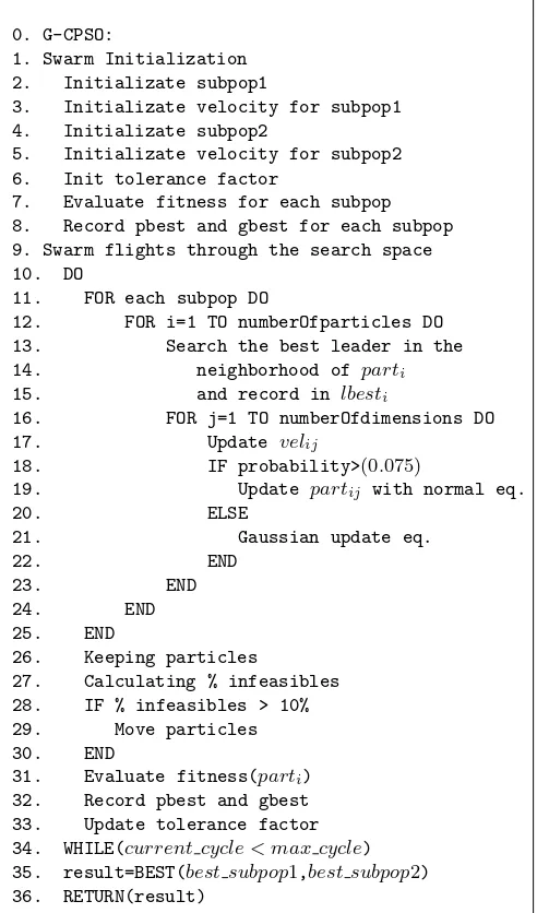
0. G-CPSO:
1. Swarm Initialization 2. Initializate subpop1
3. Initializate velocity for subpop1 4. Initializate subpop2
5. Initializate velocity for subpop2 6. Init tolerance factor
7. Evaluate fitness for each subpop 8. Record pbest and gbest for each subpop 9. Swarm flights through the search space 10. DO
11. FOR each subpop DO
12. FOR i=1 TO numberOfparticles DO 13. Search the best leader in the 14. neighborhood of parti
15. and record in lbesti
16. FOR j=1 TO numberOfdimensions DO 17. Update velij
18. IF probability>(0.075)
19. Update partij with normal eq.
20. ELSE
21. Gaussian update eq.
22. END
23. END
24. END 25. END
26. Keeping particles
27. Calculating % infeasibles 28. IF % infeasibles > 10% 29. Move particles 30. END
31. Evaluate fitness(parti)
[image:5.595.186.432.167.585.2]32. Record pbest and gbest 33. Update tolerance factor 34. WHILE(current cycle < max cycle) 35. result=BEST(best subpop1,best subpop2) 36. RETURN(result)
number of points (Pts) desired in the solution Pareto set. The number of eval-uations is calculated asPts × c × particles. Being particles the number of
particles in the population of the G-CPSO procedure.Solutionis the set with the Pareto front found.
The selection off1orf2 as the first function to be optimized is arbitrary. In our case,f1 was always taken as the objective function to optimize.
0. Epsilon-Constraint with PSO: 1. Solution=∅
2. ub=f2(G-CPSO(f1,c))
3. lb=f2(G-CPSO(f2,c))
4. t=0.05(ub-lb) 5. δ= (ub-lb)/Pts 6. ub=ub+t 7. lb=lb-t 8. ǫ=lb
9. WHILE ǫ≤ ub DO 10. x=G-CPSO(f1,ǫ,c)
11. IF x is nondominated in Solution THEN 12. delete all dominated by x
13. add x to Solution 14. ǫ=ǫ+δ
[image:6.595.190.427.206.402.2]15. RETURN Solution
Fig. 2.Pseudocode of our Epsilon-Constraint Approach.
3.3 Enhancing the Quality of the Pareto front obtained
Solving hard multiobjective functions can result computationally expensive, even using epsilon-constraint method. On the other hand, we believe that Pareto fronts with less of 50 points can not be adequate. For that, we consider that keep the Pts value low is a priority, and propose to use a simple interpolation technique to cover a larger area of the true Pareto front. We interpolate the solution set obtained with the algorithm of Figure 2, with a cubic splines in-terpolation [12]. Finally, we return the set so obtained as final solution of our approach.
4
Test Functions and Metrics
of evaluations is not restricted. For that, we want to test these and conclude if our approach is a viable alternative to solve them.
These two problems were proposed by Okabe [14], referenced as OKA1 and OKA2. They have 2 and 3 variables respectively, and 2 objective functions. The geometry of their optimal sets is nonlinear and strongly biased to the opposite side of the Pareto front.
We selected the following metrics to evaluate the performance of our algorithm: a. Two Set Coverage (CS) metric [20], that is an indicator of how much a set covers or dominates another one. Considering X and Y two Pareto fronts, a value of CS(X,Y)=1 means that all points in X dominate or are equal to those in Y. A CS(X,Y)=0 indicates the opposite. Note that CS(X,Y) it is not the same that CS(Y,X), so both might be calculated.
b. Spread indicator (Spr), a diversity metric that measures the extend of spread achieved among the obtained solutions [4]. A value of Spr=0 indicates that the obtained front has an ideal distribution.
c. The Inverted Generational Distance [15] (IGD), a quality indicator that mea-sures how far the elements are in the Pareto optimal set from those in the set of nondominated vectors found. A IGD=0 indicates that all the generated elements are in the Pareto true front.
5
Experimental Setup
In order to compare the results obtained by our approach, we use the results obtained with NSGA-II [4], which is an algorithm representative of the state of the art in the multiobjective optimization area.
We ran both algorithms for 15,000 and 25,000 fitness function evaluations for OKA1 and OKA2, respectively. We had to increase the evaluation number for OKA2 because is a more hard problem than OKA1. We aimed to obtain a set of 50 points in the final Pareto fronts.
The parameters adopted here are the same proposed in [1] for G-CPSO: 10 parti-cles, size of neighborhood=3, c1=c2=c3=1.8, w=0.8 and flip-probability=0.075. The parameters for NSGA-II were the suggested by the authors: population=50, probability of crossover=0.9, distribution index for crossover=15, probability of mutation=1/number−variables and the distribution index for mutation=20. We executed 30 independent runs with both algorithms. The means (and stan-dard deviations) for each problem are showed in Table 1 and Table 2. Note that our approach is referenced asǫ−G-CPSO.
Table 1.Averaged metric values for OKA1. Means (and standard deviations).
Metric ǫ−G-CPSO NSGA-II
Spread 0.6978(0.2200) 0.7079(0.0630)
IGD 0.0024(0.0006) 0.0043(0.0019)
CS(ǫ−G-CPSO,NSGA-II) 0.5712(0.0861) -CS(NSGA-II,ǫ−G-CPSO) - 0.2356(0.0730)
Table 2.Averaged metric values for OKA2. Means (and standard deviations).
Metric ǫ−G-CPSO NSGA-II
Spread 0.9190(0.2624) 1.1805(0.1285)
IGD 0.0057(0.0025) 0.0116(0.0040)
CS(ǫ−G-CPSO,NSGA-II) 0.6332(0.2980) -CS(NSGA-II,ǫ−G-CPSO) - 0.2287(0.1505)
NSGA-II. The IGD are very small for our approach (many points in our solution are in the true Pareto front) and are better than those obtained by NSGA-II. To illustrate the performance of the algorithms, Figures 3 and 4 show the results of a single run for each problem.
6
Conclusions and Future Work
We have introduced a new proposal to work on hard multiobjective optimization problems using a mathematical technique hybridized with a particle swarm op-timizer. The performance of our approach turned out to be satisfactory in this preliminary study, even more, in both cases tested outperformed the results of NSGA-II algorithm.
Our conclusion is that the results are promising and this fact encourages us to continue working in this address, considering additional hard multiobjective problems with two and three objective functions.
Acknowledgments
[image:8.595.184.432.268.354.2]Fig. 3.Pareto fronts for OKA1.
[image:9.595.141.474.400.635.2]References
1. L. Cagnina, S. Esquivel, and C. Coello Coello. A bi-population pso with a shake-mechanism for solving constrained numerical optimization. In IEEE Congress on Evolutionary Computation - CEC2007, pages 670–676, Singapore, 2007.
2. C. Coello Coello, G. Lamont, and D. Van Veldhuizen.Evolutionary algorithms for solving multi-objective problems. Springer, 2007. ISBN 978-0-387-33254-3. 3. J. L. Cohon and D. H. Marks. A review and evaluation of multiobjective
program-ming techniques. Water Resources Research, 11(2):208–220, 1975.
4. K. Deb, A. Pratap, S. Agrawal, and T. Meyarivan. A fast and elitist multiobjective genetic algorithm: NSGA-II. IEEE Transactions on Evolutionary Computation, 6(2):182–197, 2002.
5. R. Eberhart and J. Kennedy. A new optimizer using particle swarm theory. In Proceedings of the Sixth International Symposium on Micro Machine and Human Science, MHS’95, pages 39–43, Nagoya, Japan, October 1995. IEEE Press. 6. J. Grobler and A. P. Engelbrecht. Hybridizing PSO and DE for improved vector
evaluated multi-objective optimization. E-Commerce Technology, IEEE Interna-tional Conference on, 0:1255–1262, 2009.
7. Y. Y. Haimes, L. S. Lasdon, and D. A. Wismer. On a bicriterion formulation of the problems of integrated system identification and system optimization. IEEE Transaction on Systems, Man, and Cybernetics, 1(3):296–297, 1971.
8. J. Horn. Multicriterion decision making. Handbook of Evolutionary Computation, 1:F1.9:1–F1.9:15, 1997.
9. W. Jingxuan and W. Yuping. Multi-objective fuzzy particle swarm optimization based on elite archiving and its convergence. Journal of Systems Engineering and Electronics, 19(5):1035–1040, 2008.
10. X. Lin and H. Li. Enhanced pareto particle swarm approach for multi-objective optimization of surface grinding process.2007 Workshop on Intelligent Information Technology Applications, 2:618–623, 2008.
11. C. Liu. New dynamic constrained optimization pso algorithm. In ICNC ’08: Proceedings of the 2008 Fourth International Conference on Natural Computation, pages 650–653, Washington, DC, USA, 2008. IEEE Computer Society.
12. S. McKinley and M. Levine. Cubic spline interpolation. Math 45: Linear Algebra. 13. K. M. Miettinen. Nonlinear Multiobjective Optimization. Kluwer Academic
Pub-lishers, 1999. Boston, Massachusetts.
14. T. Okabe. Evolutionary Multi-Objective Optimization - On the Distribution of Offspring in Parameter and Fitness Space. PhD thesis, Bielefeld University, 2004. 15. D. A. Van Veldhuizen and G. B. Lamont. Multiobjective evolutionary algorithm research: A history and analysis. Technical report, Dept. Elec. Comput. Eng., Graduate School of Eng., Air Force Inst. Technol, Wright-Patterson, AFB.OH, 1998. TR-98-03.
16. D. A. Van Veldhuizen and G. B. Lamont. Multiobjective evolutionary algorithms: Analysing the state-of-the-art. Evolutionary Computation, 7(3):1–26, 2000. 17. Y. Wang and Z. Cai. A hybrid multi-swarm particle swarm optimization to solve
constrained optimization problems.Frontiers of Computer Science in China, 2009. 18. Y. Wang and Y. Yang. Particle swarm optimization with preference order ranking
for multi-objective optimization. Inf. Sci., 179(12):1944–1959, 2009.
19. E. Zahara and C. Hu. Solving constrained optimization problems with hybrid particle swarm optimization. Engineering Optimization, 40, 2008.