Parallel ant algorithms for the minimum tardy task problem

Parallel Ant Algorithms for the Minimum Tardy Task Problem

Enrique Alba , Guillermo Leguizam´on

✁

, and Guillermo Ordo˜nez

✁

✂

Universidad de M´alaga,

Complejo Tecnol´ogico - Campus de Teatinos, 29071 M´alaga, Spain

eat@uma.es

✄

Universidad Nacional de San Luis, Ej´ercito de los Andes 950, (5700) San Luis, Argentina

legui@unsl.edu.ar

Abstract. Ant Colony Optimization algorithms are intrinsically distributed algorithms where independent agents are in charge of building solutions.Stigmergyor indirect communication is the way in which each agent learns from the experience of the whole colony. However, explicit communication and parallel models of ACO can be implemented directly on different parallel platforms. We do so, and apply the resulting algorithms to the Minimum Tardy Task Problem (MTTP), a scheduling problem that has been faced with other metaheuristics, e.g., evolutionary algorithms and canonical ant algorithms. The aim of this article is twofold. First, it shows a new instance generator for MTTP to deal with the concept of “problem class”; second, it reports some preliminary results of the implementation of two type of parallel ACO algorithms for solving novel and larger instances of MTTP.

keywords:ant colony optimization, parallel models, minimum tardy task problem

1

Introduction

The ant colony optimization technique (Dorigo et al. [6]) is a new meta-heuristic for hard combina-torial optimization problems. An ant algorithm, that is, an instance of the ant colony optimization meta-heuristic, is basically a multi-agent system where low level interactions among simple agents (calledartificial ants) result in a complex behavior of the whole system. Ant algorithms have been in-spired by colonies of real ants, which deposit a chemical substance (calledpheromone) on the ground. This substance influences the choices they make: the larger the amount of pheromone on a particu-lar path, the particu-larger the probability that an ant selects the path. Artificial ants, in ant algorithms, are stochastic construction procedures that probabilistically build a solution by iteratively adding prob-lem components to partial solutions by taking into account (i) heuristic information from the probprob-lem instances being solved, if available, and (ii) pheromone trails which change dynamically at run-time to reflect the acquired search experience.

Traditional applications of the ACO approach in combinatorial optimization problems include the Traveling Salesperson Problem, the Quadratic Assignment Problem, as well as the Job Shop Schedul-ing, Vehicle RoutSchedul-ing, Graph Coloring and Telecommunication Network Problem [6]. More recently, promising results were reported in [10, 9] from the application of a new version of an Ant System to the Multiple Knapsack and to the Maximum Independent Set Problems, two examples of subset problems with constraints, for which an ant colony algorithm was first applied. Also, the ant approach for subset problems was successfully applied to the Minimum Tardy Task Problem in the past [8].

just summarize some parallel implementations and models found in the literature (not in an exhaustive manner, of course). Additional revisions of this topic for interested readers are [16], [17], and [7].

Up to now, a few papers deal with parallel ACO. Some parallel models can be found in [3] (parallel AS for TSP), or in [4, 5] (sync master-slave models and async distributed AS search). Also, there exist general works on parallel strategies like the one in [21] (independent versus coupled search), and several parallel models targeted to solve a complex application, like references [15], [22] and [11].

This work aims at evaluating the application of two main parallel ant algorithms to the minimum tardy task problem. Some variations on the model and a detailed discussion on the problem instances are used to achieve the main aim of this article.

The paper is organized as follows. Section 2 describes the minimum tardy task problem. The proposed generator of MTTP instances is presented in Section 3 including a brief discussion about the difficulty of the set of instances generated and used here. Section 4 features the main characteristics of the ant algorithms for subset problems, and a small example of the process for building a solution for MTTP. In Section 5 the parallel algorithms implemented for our experiments are described. The experiments and their results are discussed in Section 6. Finally, conclusions and further work are drawn in Section 7.

2

The Minimum Tardy Task Problem (MTTP)

The minimum tardy task problem (MTTP) is an NP-hard task-scheduling problem [13]. It follows a formal definition of MTTP [20]:

Problem instance:

Tasks: 1 2 . . . ☎ ,

✆ ✝

0

Lengths: ✞ ✞

✁

. . . ✞✠✟ , ✞✠✡

✝

0 Deadlines: ☛ ☛

✁

. . . ☛☞✟ , ☛☞✡

✝

0

Weights: ✌ ✌

✁

. . . ✌✍✟ , ✌✍✡

✝

0

Feasible solution: A one-to-one scheduling function ✎ defined on ✏✒✑✔✓ , ✎✖✕✗✏✙✘✛✚ ✜✣✢✥✤✧✦✩★✫✪ that

satisfies the following conditions for all✆✭✬✯✮✱✰

✏ :

1. If ✎✳✲ ✆✯✴✶✵

✎✷✲ ✮✫✴

then ✎✳✲ ✆✸✴✺✹

✞✠✡✼✻✽✎✳✲ ✮✾✴

which insures that a task is not scheduled before the completion of an earlier scheduled one.

2. ✎✳✲ ✆✸✴✷✹

✞✠✡✿✻✒☛☞✡ which ensures that a task is completed within its deadline.

Objective function: The tardy task weight

❀ ❁✔❂

✡❄❃❆❅✗❇✾❈

✌✍✡ , which is the sum of the weights of unscheduled tasks.

Optimal solution: The schedule✏ with the minimum tardy task weight

❀

.

A subset ✏ of ✓ is feasible if and only if the tasks in ✏ can be scheduled in increasing order

by deadline without violating any deadline [20]. If the tasks are not sorted in that order, one needs to perform a previous polynomially executable preprocessing step in which the tasks are ordered in increasing order of deadlines, and renamed such that☛ ✻✒☛

✁

✻❊❉❋❉❋❉●✻✒☛☞✟✾❍

Example: Consider the following problem instance of the minimum tardy task problem:

Tasks: 1 2 3 4 5 6 7 8

Lengths: 2 4 1 7 4 3 5 2

Deadlines: 3 5 6 8 10 15 16 20

Weights: 15 20 16 19 10 25 17 18

a) ✏

❁

✦❏■ ✬▲❑▼✬❖◆✫✬▲P

✪ is a feasible solution and the schedule is given by:✎✳✲◗■ ✴ ❁

★

✬

✎✳✲

❑❘✴ ❁❚❙ ✬

✎✳✲ ◆☞✴ ❁

❑

and✎✳✲ P❘✴

❁❱❯

❍ The objective function value amounts to

❂

✡✠❃❆❅✗❇✾❈ ✌✍✡

❁

✌

✁

✹

✌✍❲

✹

✌❨❳

✹

✌❬❩❭❍

b) ✏❫❪

❁

✦

❙

✬▲❑▼✬✭❴●✬▲P▼✬▲❵

✪ is infeasible. We define✎✳✲

❙

✴

❁

★ , and task 2 finishes at time★

✹

✞

✁

❁

❴

which is within its deadline☛

✁

❁ ◆

❍ We schedule tasks 3 at 4, i.e.✎✳✲

❑☞✴ ❁ ❴

, which finishes at✎✳✲ ❑☞✴❛✹

✞❝❜

❁ ◆

which is within its deadline ☛❏❜

❁ P

. But task 4 cannot be scheduled since✎✳✲ ❴❏✴❞✹

✞❡❲

❁ ◆❬✹ ❯❢❁

■

❙

and will thus finish after its deadline☛❏❲

❁

❵

.

3

A New Generator of MTTP Instances

A serial version of an ant algorithm for subset problems was applied successfully in [8] to several instances of MTTP. These instances have been previously used in the associated literature. This ant algorithm, called ACAsp, showed a very good performance for several instances of different sizes which were generated following the scalable procedure described in [1]. This procedure assigns the respective weight value to each task in a manner that is possible to know the optimal solution in advance. However, the resulting instances could be easily solved by constructive methods3_{guided by}

a subordinate heuristic that takes into account the benefit (given by✌❣✡✐❤❥✞✠✡) of including a task

✆

in the solution under construction.

In order to obtain arbitrarily sized and hard MTTP instances we developed a new problem gener-ator from which it is possible to tune in a controlled manner the size of the feasible search space in comparison to the whole search space4.

The interest in using problem generators in evaluating metaheuristics is of a capital importance nowadays. By using a problem generator, each time the algorithm is run it solves adifferentinstance of the problem (i.e., different numerical values are used given birth to different instances of the same complexity). Using a generator removes the opportunity to hand-tune the algorithms or to bias the results in any way to favor the evaluated algorithm. In addition, because a great deal of instances are solved in any such analysis, the conclusions can be really said to affect the problem class, not to solve individual instances, whatever their difficulty happen to be. As a conclusion, using problem generators is an important step towards a serious evaluation of new algorithms.

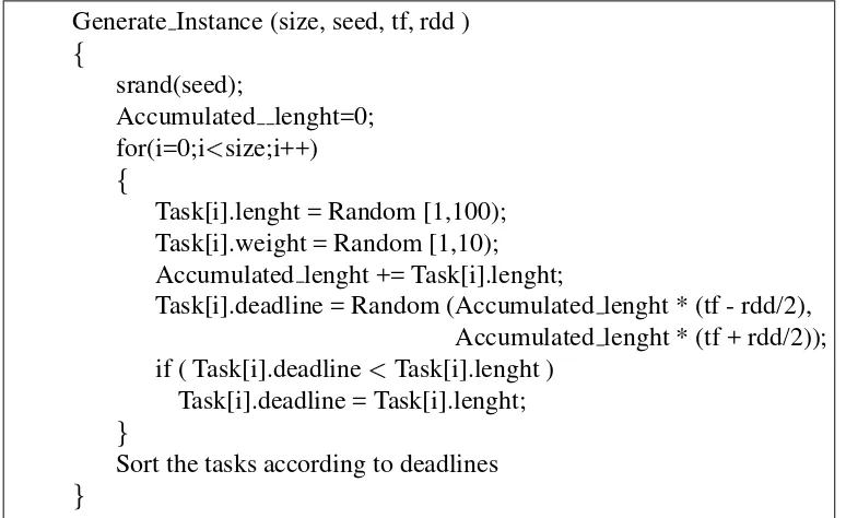
Our proposed procedure (see figure 1) is based on the algorithm used to generate instances of the Weighted Tardiness Problem found in [2]. This procedure needs four parameters: the size of the instance or number of tasks, an integer number to seed the random generator, and two additional parameters to control the tightness of the deadlines. The respective values✞❝✡ (Task[i].lenght) and✌❬✡

(Task[i].weight) are randomly obtained by using a uniform distribution from the continuous intervals

❦

■

✬

■❭★☞★♠❧ and

❦

■

✬

■❋★♠❧ respectively. Similarly, ☛❏✡ (Task[i].deadline) is obtained from the interval

5 ❦♦♥ ✡✺♣

3_{For example, greedy, random-greedy, ACO algorithms, etc.} 4

e.g., the more constrained are the deadlines, the smaller is the feasible search space. 5q✳r

Generate Instance (size, seed, tf, rdd )

✦

srand(seed);

Accumulated lenght=0; for(i=0;i✵

size;i++)

✦

Task[i].lenght = Random [1,100); Task[i].weight = Random [1,10); Accumulated lenght += Task[i].lenght;

Task[i].deadline = Random (Accumulated lenght * (tf - rdd/2), Accumulated lenght * (tf + rdd/2)); if ( Task[i].deadline ✵

Task[i].lenght ) Task[i].deadline = Task[i].lenght;

✪

Sort the tasks according to deadlines

✪

Fig. 1.Procedure ‘Generate Instance()’. Parameters tf and rdd let us control the difficulty of the instance to be generated.

✲❝s✉t✈✘①✇❥☛❏☛

✴

❤

❙ ✬

♥

✡❭♣②✲❝s✉t

✹

✇❥☛❏☛

✴

❤

❙

❧, where

♥

✡

❁ ❂

✡

③✭④

✞

③

, i.e., the accumulated length of the tasks already generated including✞❄✡;s✉t and✇♠☛❏☛ are two parameters of the procedure which represent respectively

the average tardiness factor and the relative ranges of due dates. Parameters✉t is used to calculate the

center of the above interval. More precisely, the center of the interval is

♥

✡❘♣⑤s✉t . Similarly, the interval

size is obtained by using parameter✇✩✇❥☛ in the expression

♥

✡⑥♣⑦✇♠☛✫☛ .

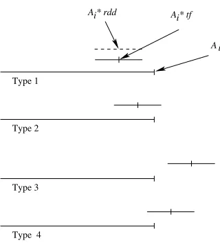
According to the setting of parameterss✉t and ✇♠☛❏☛ , instances of four types can be generated (see

figure 2):

1. s✉t

✹

✲⑧✇♠☛❏☛✾❤

❙

✴⑨✵

■ , i.e., a percentage of tasks can not be scheduled due to the highly constrained

deadlines (the lowers✉t the higher is that percentage);

2. s✉t

✵

■ ands✉t

✹

✲❝✇❥☛❏☛✫❤

❙

✴✈✝

■ , is similar to the first case, however, with a less constrained deadlines;

3. s✉t✣✘✧✲⑧✇♠☛❏☛✫❤

❙ ✴❶⑩

■ , i.e., all tasks can be scheduled since all of them will have a deadline larger than

the respective

♥

✡; and

4. s✉t

✝

■ and s✉t❷✘❸✲❝✇❥☛❏☛✫❤

❙

✴✼✵

■ , this case is similar to case 2 but even less constrained. That is,

almost all tasks can be scheduled before their respective deadlines.

Clearly, the instances of type three are not worthwile to be considered since the search space for these instances will be entirely feasible (trivial solution), i.e., the whole set of tasks can be scheduled for sure.

After✞✠✡,✌✍✡,☛☞✡ have been generated for

✆

❁

■

✬

❍❹❍

✬

☎ , the tasks of the instance are rearranged

accord-ing the increasaccord-ing values of the respective deadlines, i.e.,☛ ✻❺☛

③

✻❻❍❹❍✷✻❊☛☞✟ , where☎ represents the

A * rdd _{A * tf}

A

i i

i

Type 1

Type 2

Type 3

Type 4

Fig. 2.Four cases for deadlines generation according to the setting of parameters❼❝❽ and❾✉❿▲❿ .

3.1 Problem Complexity and Parameterstf-rdd

Since parameters s✉t and ✇♠☛❏☛ control the resulting MTTP instances, we first include a preliminary

analysis of their actual effects in the resulting instance complexity. We evaluate a simple ACO on instances obtained by using different values of such parameters on problems of the same size. The performance is measure by computing the success rate and the number of steps to locate the best known optima.

We created 10 instances by merging different values ofs✉t and✇♠☛✫☛ and performed 20 independent

runs for each one. We used a single value✇❥☛❏☛

❁

★▼❍

❙

and tested ten values of s✉t (0.1, 0.2, 0.3, 0.4,

0.5, 0.6, 0.7, 0.8, 0.9). In figure 3 we plot the results for the effort in solving (best known value as stopping criterion) instances of size 100 and 200.

0 10 20 30 40 50 60 70

0.1 0.2 0.3 0.4 0.5 0.6 0.7 0.8 0.9

Parameter tf

Iterations

100 200

We can notice that small values ofs✉t provoke the hardest instances. This scenario is not that clear

for instances of size 100. A similar conclusion can be drawn when analyzing figure 4. In this figure, the➀ axis represents the complement of the percentage of hits(100% - (#hits)).

0.00 5.00 10.00 15.00 20.00 25.00 30.00 35.00

0.1 0.2 0.3 0.4 0.5 0.6 0.7 0.8 0.9

Parameter tf

100% - (#Hits)%

100 200

Fig. 4.Values of❼❝❽ versus 100% - (#hits)%.

To analyze the influence of✇❥☛❏☛ (0.1, 0.2, 0.4) only three values of s✉t were considered to avoid

the cartesian product explosion of possibilities: (0.1 , 0.2, 0.3). In figure 5 we can see that s✉t

❁

★▼❍❹■

for instances of size 200 provokes easier instances (in terms of number of steps to locate a solution)

as ✇♠☛✫☛ increases, i.e., the larger the interval the easiest the resulting problem instances. A similar

conclusion was drawn for instances of size 100 (not shown here for room constraints).

0 5 10 15 20 25 30 35 40 45 50

0.1 0.2 0.4

Parameter rdd

Iterations

0.1 0.2 0.3

Fig. 5.Values of❾✉❿▲❿ versus effort to locate an optimum.

In summary, the complexity of the generated instances can be tuned by using small values of

s✉t and ✇♠☛❏☛ . If we compare all these instances with respect existing ones (for example see [8]) our

4

Outline of an Ant algorithm for Subset Problems

Our ant colony algorithm for a general subset problem works as follows (see [10, 9, 8] for further details). In each cycle of the algorithm ➁ ants are released to build a new solution. Each ant in the

colony builds a solution independently from the other ants. At this initial stage, all problem compo-nents are feasible6_{. Each new component is selected from the set of feasible components. After that,}

the selected component is incorporated into the solution under construction. At the same time, the set of feasible components is updated in order to eliminate all components that became infeasible after the addition of a new component to the solution. This procedure is repeated until the set of feasible components is empty. The pheromone trail levels are updated accordingly to the type of ant algorithm used.

The Ant System (AS) was the first example of an ant colony optimization algorithm to be pro-posed in the literature. However, AS was not competitive with state-of-the-art algorithms for TSP, the problem to which the original AS was applied. There exist several improvements to the original version of AS, much of them applied to the TSP. The more important improvements are: AS with an

elitist strategyfor updating the pheromone trail levels, AS➂✸➃◗✟❭➄ (a rank-based version of Ant System), ➅➇➆➉➈

-➅➋➊➍➌

Ant System (

➅➇➅

AS), and the Ant Colony System (ACS)7.

For this work we implemented an Ant Colony System (ACS). Basically, an ACS algorithm is an improved version of an AS. The ACS increases the exploitation of the information collected by the ant colony in order to guide the exploration of the search space. There exist two mechanisms to achieve such a goal. The first one uses a strongly elitist strategy to update the trail. The second one changes the original mechanism for item selection (next component to be included in the solution) by using a pseudo-random proportional rule which works as follows: with probability➎➐➏ an ant chooses the next

component✮➑✰➓➒

such as✮

❁

arg max③ ❃→➔

✦❋➣

③

✲✐s

✴

❉❥↔❏↕

③

✲✐s

✴

✪ , otherwise, the next component is chosen

according to eq.1 (similar to that used in Ant Systems).

➙

➄

③

✲✐s

✴

❁ ➣

③

✲❝s

✴

❉❋↔

③

✲❝s

✴

↕

❂✖➛

❃→➔

➣

➛

✲❝s

✴

❉❭↔

➛

✲❝s

✴

↕

(1)

where↔

③

is a heuristic value associated to component✮

;➜ that controls the importance of the above

value in the respective formula, and ➣

③

ensures that preference is given to components (tasks in the case of MTTP) that belong to solutions of high quality.➒

represents the set of feasible components with respect to the problem constraints. When➎❋➏ is close to ■ , the ACS is highly greedy, thus favoring

components which posse the best combination of large pheromone levels and heuristic values. On the other side, setting➎❭➏

❁

★ implies that the ACS behaves similarly to an AS concerning the selection

of the next component. Therefore, the value given to ➎➐➏ determines the balance between a greedy

and a probabilistic selection of the next component. Additionally, there exist local an global rules for updating the pheromone levels. The local rule (which uses a constant value) is executed after each ant makes a selection on the next component, whereas the global one is applied at the end of each iteration by using the objective value of the best solution so far[12].

Let us now present the process by which our ant algorithm builds a solution for MTTP with a particular ant. The instance considered is taken from the example of size ❵

on page 3. Initially

6_{We assume a constrained optimization problem.} 7

✏ and ➟ ✦❏■

✬ ✬▲❑▼✬➠❴▼✬❖◆✾✬▲P▼✬ ✬▲❵

✪ , i.e., the solution under construction and the set of allowed

tasks to schedule next (at the beginning, all tasks are schedulable). Next, the ’repeat’ loop starts: let us suppose that✆ ❁

■

8 _{is the next task}9 _{selected from}

➟ . Then,✏

❁

✏➑✤➡✦❏■❥✪

❁

✦❏■♠✪ ,✎✳✲➢■ ✴ ❁

★ , and

♥ ❁ ✦ ❑▼✬❖◆✾✬➠P▼✬ ❯ ✬▲❵

✪ , since✎✳✲

❙ ✴❛✹ ✞ ✁ ✝ ☛ ✁ ,✎✷✲ ❴❏✴✗✹ ✞✠❲ ✝

☛☞❲ and task ■ is already in the solution. Iteration

two, ✆ ❁ ◆

, ✏ ❁ ✏➤✤➥✦ ◆ ✪ ❁ ✦❏■ ✬▲◆ ✪ , ✎✳✲➢■ ✴ ❁ ★ , ✎✳✲ ◆❥✴ ❁➦❙

, and ➟

❁

✦

❑▼✬➠P▼✬ ❯ ✬▲❵

✪ since

◆

has been selected. Iteration three, ✆ ❁ P

, ✏ ❁ ✏⑦✤➧✦ P ✪ ❁ ✦❏■ ✬❖◆✾✬➠P ✪ , ➟ ❁ ✦ ❑▼✬ ❯ ✬➠❵

✪ , and✎✳✲◗■ ✴ ❁ ★ ✬ ✎✳✲ ◆☞✴ ❁❊❙ , and ✎✳✲ P❘✴ ❁ P

. Iteration four,✆

❁ ❑ , ✏ ❁ ✏➨✤⑦✦ ❑ ✪ ❁ ✦❏■ ✬▲❑▼✬▲◆✾✬▲P

✪ . In this case the number of task selected is

in between tasks■ and

◆

, therefore the values✎✳✲ ✮✾✴

for✮✱✰

✦

◆✾✬➠P

✪ , will change after the re-scheduling

process takes place, thus ✎✷✲◗■ ✴ ❁ ★ ✬ ✎✳✲ ❑❘✴ ❁➩❙ ✬ ✎✳✲ ◆☞✴ ❁ ❑ , ✎✳✲ P☞✴ ❁✽❯

, and ➟

❁

✦

❯ ✬➠❵

✪ . Iteration five,

✆ ❁ ❵ , ✏ ❁ ✏⑦✤➑✦ ❵ ✪ ❁ ✦❏■ ✬▲❑▼✬▲◆✾✬▲P▼✬▲❵ ✪ ,✎✳✲➢■ ✴ ❁ ★ ,✎✳✲ ❑❘✴ ❁❊❙ , ✎✳✲ ◆☞✴✉❑ ,✎✳✲ P❘✴ ❁❊❯ , ✎✳✲ ❵❘✴ ❁

■❋★ , and➟

❁ ✦ ❯ ✪ . Finally,✆ ❁➫❯ , ✏ ❁ ✏⑦✤✧✦❏■ ✬▲❑✾✬❖◆✾✬▲P▼✬ ❯ ✬▲❵ ✪ ,➟ ❁➭➝ ,✎✷✲◗■ ✴ ❁ ★ ✬ ✎✳✲ ❑❘✴ ❁❸❙ ✬ ✎✳✲ ◆☞✴ ❁ ❑▼✬ ✎✳✲ P❘✴ ❁➭❯ ✬ ✎✳✲ ❯ ✴ ❁ ■❋★ , and✎✳✲ ❵☞✴ ❁ ■ ◆ .

The feasible solution obtained is ✏

❁

✦❏■

✬➠❑▼✬❖◆✾✬▲P✾✬

❯

✬▲❵

✪ with an objective value of

❂ ✡❄❃❆❅✗❇✾❈ ✌✍✡ ❁ ✌ ✁ ✹ ✌✍❲ ❁❱❙ ★ ✹ ■❋➯ ❁ ❑

➯ . Solution✏ is equivalent to10101111if represented as a binary string.

5

Parallel Strategies for ACO Metaheuristic

In section 1 we enumerated several parallel implementations of ACO algorithms. Most of them belong to the general purpose parallelization strategies given by Randall et al.[18] according to the level at which the parallelism is exploited. For example, at a large scale, the entire search could be performed concurrently. Alternatively, parallelism can sometimes be used for the evaluation of solution elements, particularly when this evaluation is computationally expensive. However, it must be said that parallel performances can suffer when there is a large communication overhead among the processors.

Randall et al.[18] proposed an interesting classification of parallelization strategies for ACO meta-heuristic. These are: Parallel Independent Ant Colonies,Parallel Interacting Ant Colonies, Parallel Ants, Parallel Evaluation of Solution Elements, andA Combination of the two strategies mentioned above.

For our work we considered the first and second strategies, that are described in the following. Parallel Independent Ant Colonies (Strategy A or ✏❞➲ ) is an approach in which a number a sequential

ACO searches are run across the available set of processors. Each colony is differentiated in the values of key parameters. In this method, no communication is required between processors. Parallel Interacting Ant Colonies (Strategy B or ✏➍➳ ) is similar to the method above, except that an exchange

of information between colonies occurs at preset iterations. Although the description in [18] implies sharing of the pheromone trail structure of the best performing colony among all the colonies, it is possible to exchange in some way the best solutions found in each colony. Therefore, the exchange of solutions between colonies can be considered as a class of interaction between parallel ant colonies.

Strategy✏✷➲ can be easily implemented and no additional explanation is required. However,

strat-egy ✏✷➳ admits different implementations according to a particular parallel model. In this work we

considered theIsland Model, called✏⑥➵ ➳ .

The two parallel strategies studied in this paper for the ACO algorithm, i.e., ✏⑥➲ and ✏❞➵

➳ ; were

implemented using the MALLBA project library which includes two family of classes according

8

The values of➸ are given arbitrarily in order to proceed with the example.

9

to their purpose in the system. They are called provided and required respectively. The provided

classes conform the skeleton of the ACO metaheuristic, i.e., those classes that are independent of the problem at hands. On the other hand, therequired classes are specific for a particular problem (e.g., the heuristic value↔ ).

5.1 Strategy➺➼➻ ➽

This strategy is implemented by using the unidirectional ring topology for communications of the best-so-far solution which is used in MALLBA for many other EAs implemented under the island model (see figure 6). This kind of communications let us reuse many object classes already defined in MALLBA regarding a particular similarity between evolutionary and ant algorithms: they are two population based techniques.

In this island approach, the whole colony is split into ☎ sub-colonies which are distributed onto

the processors available in the network. Each sub-colony searches for solutions independently of the remaining sub-colonies by using a local pheromone trail structure. The interaction among the colonies comprises the migrations of some partial solutions in order to share the learning experience with the other sub-colonies. Although EAs and ACO metaheuristic are population based techniques, EAs

pro-0

3 2

n−1 1

Statistics

Fig. 6.Topology of communication between the sub-colonies. Additionally, there exists a node in charge of collecting the results from each sub-colony.

cess a population of solutions, whereas ant algorithms deal with a population of agents (ants) headed to build solutions. In this sense EAs are instance oriented approaches, while ant algorithms exhibit a model oriented approach[14]. Consequently, the solutions arriving to a target sub-colony are used in the local trail updating process under certain conditions, or they would be ignored. The rationale behind this mechanism is that the pheromone trail is the main building block of ACO algorithms. Therefore, the sub-colonies influence the local trail of a particular sub-colony by sending their best-so-far solutions. The migrations of solutions can be synchronous or asynchronous (both approaches can be used inside the MALLBA library). More precisely, according to the ring topology, sub-colony

✆

tries to influence the respective pheromone trail levels of the sub-colony ✲ ✆❞✹

■

✴

mod ☎ by sending

its best solutions (☎ is the number of sub-colonies in the network).

6

Experimental Evaluation of the Proposed Parallel Ant Algorithms

➶

❼❝❽➘➹✐❾➢❿▲❿→➴ Greedy %hits BestIt➷

➪♠➬❡➮❡➱❐✃⑧➱

%hits BestIt➷ ➪✩➬❡➮❡➱❒✃❝➱

(0.1,0.1) 11.51% 100.00 25.54 65.50 99.50 19.80 49.57 (0.1,0.2) 11.21% 90.50 5.28 29.76 90.00 2.96 5.92 (0.2,0.1) 19.11% 100.00 5.02 18.16 100.00 6.09 24.21 (0.2,0.2) 22.25% 100.00 13.83 45.12 100.00 19.47 60.17

Table 1.Instances of size 100.

one with 16 agents performing the corresponding cycle of the ant algorithm in parallel. Strategy ✏❫➳

includes a migration operation which will occur in a unidirectional ring topology, sending the best local solution to the neighboring sub-colony. The target sub-colony uses all the incoming solutions arrived so far plus the current local solutions for updating the pheromone trail structure. After this updating step, all the immigrants solutions are deleted.

The migration step is asynchronously performed every 5 cycles of the algorithm running on every island. We are using a network of Pentium IV processors at 2,6 GHz linked by a Fast Ether network at 100 Mbps.

Tables 1 and 2 display the results for strategies ✏❞➲ and ✏✷➳ on instances of size ■❋★☞★ and

❙

★❥★ ,

respectively. Columns #hits, BestIt, and ❮✛➳❛❰✯Ï❝ÐÒÑ◗Ð indicate (respectively) the average of the percentage

of hits over all runs, the minimum number of iteration to obtain the best value, and the associated standard deviation. Additionally, we included a column (named Greedy) which indicates the average of percentile distance from the best found, that is ✲ÔÓ①Õ❏✞✐ÖØ×♠Ù▼➂✸❰Ú❰ÔÛ✸Ü❬✘ÞÝ②×➐ß➘s✉ÓàÕ❏✞✐Ö✛×❭➲▼á❛â

✴

❤❥Ýà×➐ß❭s✉Ó①Õ✫✞✐ÖØ×❭➲●á❛â .

Clearly, the values obtained by the greedy heuristic are far from the corresponding best values from the two strategies considered. However, this preliminary results do not show any statistically significant difference between ✏✷➲ and ✏✷➳ , i.e., without and with migration, respectively. A future study should

be devoted to locate what are the exact differences between these two approaches, if any.

➾ ➚ ➾ ➪

➶

❼❝❽➘➹✐❾➢❿▲❿→➴ Greedy %hits BestIt➷

➪♠➬❡➮❡➱❐✃⑧➱

%hits BestIt➷ ➪✩➬❡➮❡➱❒✃❝➱

(0.1,0.1) 12.15% 90.50 8.35 14.65 90.00 7.33 12.56 (0.1,0.2) 12.78% 70.50 50.76 99.17 75.50 66.38 116.10 (0.2,0.1) 22.05% 94.00 35.10 81.78 93.00 38.15 96.24 (0.2,0.2) 23.37% 90.50 38.86 94.35 88.50 35.16 87.21

Table 2.Instances of size 200.

We carried out an additional experiment by changing the way in which the updating process of pheromone trail is achieved in ✏➍➳ . In this case, the only incoming solutions that are included in the

An additional experiment is also analyzed in which we launched a smaller number of ants on each sub-colony. In this case, we changed the size of the sub-colony from ❵

to ❴

. Figure 7 shows the behavior of strategies ✏✷➲ and ✏✷➳ under this condition, and some variations: ✏❞➲ , ✏✷➳ , and ✏❞➳

✁

. This figure shows the complementary percentage of hits (averaged on all instances tested of size 100 and 200). ✏✷➲ is similar to ✏✷➲ except in that the size of each sub-colony is

❴

; ✏➍➳ (

❵

ants for each sub-colony) and✏➍➳

✁

(❴

ants for each sub-colony) are the versions of✏⑥➳ in which are only considered

in the updating process the incoming solutions that are better than the best so far local solution.

9.25

9.1875 9.1875

8.875

8.4375

8 8.2 8.4 8.6 8.8 9 9.2 9.4

SA SA1 SB SB1 SB2

Experiments

100% - (#Hits)%

Fig. 7.Comparison of strategies

➾✩➚

and

➾✩➪

, and some variations of them.

When comparing✏✷➲ against✏✷➲ we can observe a slight increment in the number of hits. On the

other hand, strategies✏➍➳ and✏✷➳

✁

performed more efficiently than✏➍➳ due to the change in the policy

in which we only use incoming solutions if they are better than the best local ones (elitism is worth while in replacement). Additionally, it can be observed a further improvement when comparing ✏ã➳

✁

against✏✷➳ , i.e., when the number of ants in each sub-colony is reduced.

7

Conclusions

In this article we have included a detailed study of a problem generator for the MTTP scheduling problem as well as we analyzed several strategies for developing new parallel models of search with ACO algorithms. Our conclusions show that the resulting complexity of instances can be tuned at will, what allows us to perform meaningful tests on the class family of problems like MTTP. We have explained and modelled the behavior of the generator in terms of two parameters to clearly guide future research in this field.

Future works will surely include a more detailed analysis of the new instances generator, as well as characterizing the behavior of the parallel strategies already implemented here. Also, new parallel models such as a Master/Slave algorithm is of interest in the quest for more efficient optimization tools for complex problems.

References

1. E. Alba and S. Khuri. Applying evolutionary algorithms to combinatorial optimization problems. volume I, Part II ofLecture Notes in Computer Science, pages 689–700. Springer-Verlag, Berlin, Heidelberg, 2001.

2. J. E. Beasley. OR-Library: Distributing test problems by electronic mail. Journal of the Operational Research Society, 41(11):1069–1072, 1990.

3. M. Bolondi and M. Bondaza. Parallelizzazione di un Algoritmo per la Risoluzione del Problema del Commesso Viaggiatore. Master’s thesis, Politecnico di Milano, Dipartamento di Elettronica e Informazione, 1993.

4. B. Bullnheimer, G. Kotsis, and C. Strauß. Parallelization Strategies for the Ant System. Technical Report 8, Unervisty of Viena, October 1997.

5. B. Bullnheimer, G. Kotsis, and C. Strauß. Parallelization Strategies for the Ant System. In R. De Leone, A. Murli, P. Pardalos, and G. Toraldo, editors,High Performance Algorithms and Software in Nonlinear Oprimization, volume 24 ofApplied Optimization, pages 87–100. Kluwer, 1998.

6. F. Glover D. Corne, M. Dorigo.New Ideas in Optimization. McGrawHill, 1999.

7. M. Dorigo and T. St¨utzle. Handbook of Metaheuristics, volume 57 ofInternational Series In Operations Research and Manage-ment Science, chapter 9.-The Ant Colony Optimization Metaheuristic: Algorithms, Applications, and Advances, pages 251–285. Kluwer Academic Publisher, 2003.

8. G. Ordo˜nez E. Alba, G. Leguizam´on. Evolutionary algorithms for the minimum tardy task problem. InProceedings of the International Conference on Computer Science, Software Engineering, Information Technology, e-Business, and Applications, pages 401–413, Rio de Janeiro, Brasil, 2003.

9. M. Sch¨utz G. Leguizam´on, Z. Michalewicz. An ant system for the maximum independent set problem. InProceedings of the 2001 Argentinian Congress on Computer Science, pages 1027–1040, El Calafate, Argentina,, 2001.

10. Z. Michalewicz G. Leguizam´on. New version of ant system for subset problems. InProceedings of the 1999 Congress on Evolutionary Computation, pages 1459–1464, Piscataway, NJ., 1999. IEEE Press.

11. L. M. Gambardella, ´E. D. Taillard, and G. Agazzi. MACS-VRPTW: A Multiple Ant Colony System for Vehicle Routing Problems with Time Windows. In D. Corne, M. Dorigo, and F. Glover, editors,New Ideas in Optimization, pages 63–76. McGraw-Hill, 1999.

12. T. St¨utzle M. Dorigo. The ant colony optimization metaheuristic: Algorithms, applications, and advances. Technical Report IRIDIA/2000-32, IRIDIA Universite Libre de Bruxells, Belgium, 2000.

13. D. S. Johnson M. R. Garey. W. H. Freeman and Co., San Francisco, CA, 1979.

14. N. Meuleau M. Zlochin, M. Birattari and M. Dorigo. Model-based search for combinatorial optimization. Technical report, TR/IRIDIA/2001-15, 2001.

15. R. Michel and M. Middendorf. An Island Model Based Ant System with Lookahead for the Shortest Supersequence Problem. In A. E. Eiben, T. Back, M. Schoenauer, and H.-P. Schwefel, editors,Fifth International Conference on Parallel Problem Solving from Nature (PPSN-V), volume 1498 ofLecture Notes in Computer Science, pages 692–701. Springer-Verlag, 1998.

16. M. Middendorf, F. Reischle, and H. Schmeck. Information Exchange in Multi Colony Ant Algorithms. In J. Rolim et al., editor,

Fifteenth IPDPS Workshops, volume 1800 ofLecture Notes in Computer Science, pages 645–652. Springer-Verlag, 2000. 17. M. Middendorf, F. Reischle, and H. Schmeck. Multi Colony Ant Algorithms.Journal of Heuristic, 8:305–320, 2002.

18. M. Randall and A. Lewis. A parallel implementation of ant colony optimization. Jounal of Parallel and Distributed Computing, 62:1421–1432, 2002.

19. T. B¨ack S. Khuri and J. Heitk¨otter. An evolutionary approach to combinatorial optimization problems. InProceedings of the 22nd Annual ACM Computer Science Conference, pages 66–73. ACM Press, NY., 1994.

20. D.R. Stinson. An Introduction to the Design and Analysis of Algorithms. The Charles Babbage Research Center,, Winnipeg, Manitoba, Canada, 2nd edition edition, 1987.

21. T. St¨utzle. Parallelization Strategies for Ant Colony Optimization. In R. De Leone, A. Murli, P. Pardalos, and G. Toraldo, editors,High Performance Algorithms and Software in Nonlinear Oprimization, volume 24 ofApplied Optimization, pages 87– 100. Kluwer, 1998.