A combination of spatiotemporal ica and euclidean features for face recognition

A Combination of Spatiotemporal ICA and Euclidean Features for

Face Recognition

Jiajin Lei, Tim Lay, Chris Weiland and Chao Lu

Department of Computer and Information Sciences, Towson University 8000 York Road Towson, MD 21252, USA

Email: clu@towson.edu

Abstract

ICA decomposes a set of features into a basis whose components are statistically independent. It minimizes the statistical dependence between basis functions and searches for a linear transformation to express a set of features as a linear combination of statistically independent basis functions. Though ICA has found its application in face recognition, mostly spatial ICA was employed. Recently, we studied a joint spatial and temporal ICA method, and compared the performance of different ICA approaches by using our special face database collected by AcSys FRS Discovery system.In our study, we have found that spatiotemporal ICA apparently outperforms spatial ICA, and it can be much more robust with better performance than spatial ICA. These findings justify the promise of spatiotemporal ICA for face recognition.In this paper we report our progress and explore the possible combination of the Euclidean distance features and the ICA features to maximize the success rate of face recognition.

Keywords

:

1.

INTRUDUCTION

Face recognition is one of the most successful applications of image processing and analysis, and it has become one of the major topics in the research areas of machine vision and pattern recognition in the recent years. The applications can be seen in, but not limited to, the following areas: access control, advanced human-computer interaction, video surveillance, automatic indexing of images, video database and etc. In reality the process of face recognition is performed in two steps: (1) feature extraction and selection; and (2) classification of objects. These two steps are mutually related. Although the performance of classifier is crucial, a successful face recognition methodology may also depend heavily on the particular choice of features used by the classifier. So as far as face recognition is concerned, much effort has been put on how to extract and select the representative features [1]. Feature extraction and selection involve the derivation of salient features from the raw input data for classification and provide enhanced discriminatory power. Various kinds of methods have been proposed in the literatures [1]. Among them statistical techniques, such as principle component analysis (PCA), independent component analysis (ICA), have been widely used for face recognition. These techniques represent a face as a linear combination of low rank basis images. They employ feature vectors consisting of coefficients that are obtained by simply projecting facial images onto a set of basis images [2]. The practice proved that statistical method offers much more robustness and flexibility in terms of handling variations in image intensity and feature shapes. PCA uses eigenvectors with the largest eigenvalues to obtain a set of basis functions such that the original function can be represented by a linear combination of these basis functions [3]. The basis functions found by the PCA are uncorrelated, i.e. they cannot be linearly predicted from each other. However, higher order dependencies still exist in the PCA and, therefore, the basis functions are not properly separated [4]. ICA is a method that is sensitive to high-order relationship [5, 6]. By using ICA we can explore the important information hidden in high-order relationship among the basis functions. On the other hand Euclidean features are extracted from distances between certain important points on the face. This technique takes the advantage of the fact that different people have different face shape. But how to precisely locate the face organs is a big challenge.

movements. In this study a comparison of performances among different face recognition approaches has been made. And we also explore the possible combination of the Euclidean distance features and the spatiotemporal ICA features to maximize the success rate of face recognition.

2.

THE FACE ORGAN LOCALIZATION AND EUCLIDEAN FEATURE

COMPUTATION

Feature based face recognition seeks to extract, from a face image, a set of numerical characteristics that can uniquely identify that face. Our proposed feature set is based upon the physical distances between common points of the face. In our study two features were chosen. The first feature was calculated by obtaining the distance between the centers of the eyes and the distance from the center of the left eye to the center of the mouth. These two values were then used to form a ratio in order to normalize for variance in the scaling of each image. The second feature was determined symmetrically with the center of the right eye. The third feature was extracted by making a ratio of the distance between two eyes and distance from the mouth to the middle point of two eyes.

To obtain the centers of the eyes and the mouth, a number of image processing methods were employed. In order to find the eyes, pattern matching was used to locally identify possible eyes. Specifically, the light to dark to light contrast of the pupils and eyelashes was looked for in the original grayscale image. All areas exuding this appearance were highlighted for closer scrutiny in a more global pattern-matching scheme after all potential eyes within a certain area were highlighted.

Figure 1. Identify eyes on a face

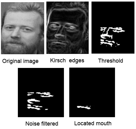
Kirsch edges Threshold Original image

Located mouth Noise filtered

Figure 2. Finding the month on a face

the same level. These two points were chosen as the approximate center of the eye, and everything not within a short distance of these areas was erased from the image. The procedures can be seen from Figure 1.

To find the mouth, a kirsch edge detection [8] filter was applied to the preprocessed grayscale image. The image had its edges removed and was then threshed based on the distribution of its histogram. The threshold value was set at the 80th percentile of the gray distribution. The mouth is one of the most contrasting features of the face, and thus with kirsch edge detection, it is featured more brightly than most parts of the face. The image was divided into small blocks in order to search for thin vertical lines and remove them as noise. The next step was to search through the binary image and obtain the characteristics of each cohesive group of remaining pixels. Objects were matched to a predefined notion of what a mouth could be, based on height verse width and area. The best matching group of pixels was taken as the mouth. The procedures of finding the month on a face are illustrated in Figure 2.

Obviously the above algorithms have their own problems and weaknesses. These revolve around alterations to the face and large variances in lighting. Dark framed glasses or glasses with any significant glare resulted in erroneous measurements. Asymmetrical facial expressions also resulted in off measurements, especially when the center of the mouth was shifted. Mustaches extending over the mouth also resulted in errors finding and reading the whole of the mouth. When part of the face was cast in a heavy shadow, unsatisfactory features were obtained. Because of these problems it is hard to use these features exclusively for classification. Combination with other features is necessary.

3.

SPATIAL ICA AND SPATIOTEMPORAL ICA FOR FACE RECOGNITION

ICA is a statistical data processing technique to de-correlate the high order relationship of input. It was originally used for blind source separation (BSS). The basic ideal behind is to represent a set of random variables using basic functions, where the components (basic functions) are statistically as independent as possible. The observed random data (signal) X= (x1, x2, ..., xm)T can be linear combination of independent components (signals) S = (s1, s2, ..., sn)T. We

may express the model as

X = AS, (1) where A is an unknown constant matrix, called the mixing matrix. In feature extraction the columns of A represent features, and si is the coefficient of the ith feature in the data vector X. Several methods for estimation of this model

have been proposed [9, 10]. Here we used fixed-point fast ICA algorithm for independent components (ICs) estimation [11].

3.1 Spatial ICA

If we concatenate a 2-D face image column-wisely, it can be represented as a 1-D signal (space-varying signal) as shown in Figure 3. Thus, a single face image becomes one entry in matrix X of (1). In face recognition, the first step is to find the ICs as well as A or its inverse W as in (2) from X by using an ICA algorithm. Each IC component can also be represented by an image. Figure 4 illustrates the procedure, and Figure 5 shows some samples of ICs.

(2)

X, * W C~ I =

(A) (B)

IC

~ X

W

IC = W * X ~

Face images Learned

weights Outputs

Figure 4. Estimate a set of ICs using ICA algorithm Figure 5. Some examples of spatial ICs

After ICs have been obtained, any observed new face image can be represented by linear combination of these ICs with a coefficient vector A as illustrated in Figure 6, and expressed in (3):

) 3 (

1 ( , ),

) ,

( ∑

=

= N

n AnICn x y y

x k X

where (A1, A2, ..., An)= A. The vector A is the desirable feature set of the observed image and will be used for classification.

3.2 Spatiotemporal ICA

Basically, spatiotemporal ICA shares the similar ideal with spatial ICA, but using an image sequence instead of a single image as operating unit. The face image sequence contains the features in both the space-domain and the time-domain. The goal of the spatiotemporal approach is to add time-domain feature into spatial 2-D feature set. So an entry in the X contains multiple images. A typical temporal image sequence is presented in Figure 7.

Figure 7. A sample of a face image sequence Figure 6. Representation of observed image with ICs

Figure 9. Representation of observed image sequence

with spatiotemporal ICs

Similar to the spatial ICA, spatiotemporal ICs can be obtained by using joint spatial and temporal algorithm. That is the entries of X in (1) are image sequences. Spatiotemporal ICs are also sequences. Figure 8 illustrates an example of spatiotemporal ICs, where each sequence consists of 12 images.

Observed face image sequences can be represented by the spatiotemporal ICs as illustrated in Figure 9 and expressed with

) 4 (

1 ( , , ),

) , ,

( ∑

=

= N

n AnICn x y t t

y x k X

where (A1, A2, ..., An)= A. Notice in (4) that the time feature has been included, which means more information is added in this model with respect to spatial ICA.

4.

LOCALIED ICA

With respect to PCA, ICA is spatially more localized [2, 6]. But it does not display perfectly the local characteristics and still uses the whole face information for operation if the input is with entire face images. Actually to recognize a person, ICA only bases on the important and valuable part of face information, such as eyes, mouth, and nose. If the whole face information is used, it may not add any more help. On the other hand, it may “dilute” the essential ones and makes performance deteriorated. So additional localization constraints should be imposed on ICA for better performance. For this purpose we take the advantage of the fact that eyes and mouth can be localized by the algorithm established in section 2. After positions of eyes and mouth have been found, a certain size of patches around eyes and mouth are respectively dug out. These two patches are concatenated together into a vector as the operation unit for matrix X of (1).

5.

AcSys FRS DISCOVERY SYSTEM AND FACIAL DATABASE PREPARATION

Face database used in this work was produced by AcSys FRS Discovery System, which is powered by HNet technology and developed by AcSys Biometrics Corp., Canada. The System, which is not just a video camera, can track precisely the human face and store a sequence of face images in real time. The purpose of our study is to consider complicated situations, such as different face expressions, face side movements, and other variations (such as with glasses) in the image sequences. The AcSys FRS system can help us to achieve this goal, while other commercially available database cannot. Figure 10 shows the main display screen of the system. Using the functions provided by the system, we can customize and take the sequential face images for different purposes. In this study, two facial datasets have been collected, one with less variation (dataset 1), and the other one with more changes in terms of face expressions and head side movements (dataset 2). For each person 200 face images were sequentially recorded for each dataset. Every face image was manually cropped to 112-by-92 pixel size.

Figure 10. FRS main screen

6.

THE EXPERIMENTS

image signal vector can become 12x112x92=123648, which is impracticable in terms of computational speed. To reduce the dimension we resized all the face images to 31-by-21 pixels. For each person 12 image sequences were produced in the following way. In the 200 image long sequence, we randomly choose a starting point, and took the following 12 images as an image sequence like given in Figure 7. For experiments of spatial ICA, localized ICA, and Euclidean features, 20 facial images were randomly picked from 200 images for each individual. In localized ICA, the patch sizes are 20-by-40 for eyes and 20-by-20 for month. For each experiment, we used half of the dataset (6 sequences for spatiotemporal ICA, 10 images for the others) for training and the remaining half for testing.

As mentioned earlier, in order to apply ICA algorithms to 2-D images, we concatenate rows of a 2-D image into a vector. The concatenated face image (space-varying) shares the same syntactic characteristics to regular time-varying signal (see Figure 3). This ensures that ICA can be applied to face image data [12]. After matrix X has been constructed with multi-image vectors, we also apply data normalization to eliminate the variation of images. Independent components (ICs) were estimated using training dataset. With the estimated ICs each observed new face image (sequence) can be represented by variant linear combination of ICs as building blocks. The variation is reflected in the amplitudes of coefficients of ICs (that is rows of matrix A), which can be found by

A = X * ICs-1 , (5)

where X is the new image (sequence) matrix (multi-images or image sequences). This matrix A contains representing features of the images (or image sequence). We used it as input data set for classification. For the purpose of performance evaluation, the numbers of ICs (features) from 2 to 200 with 10 as steps were respectively estimated. Classification was done on all of these numbers of features respectively. We calculated 3 Euclidean features for each image. Classification was conducted only once for this experiment.

We also explored performance of feature set combined from ICA features and Euclidean features. For this purpose we just appended Euclidean features to ICA feature space and repeated the above procedures. It must be noted all the experiments were conducted on both dataset1 and dataset2 parallelly.

In our experiments, linear Bayes normal classifier (LDC) and k-nearest neighbor (KNN) classifier [13] were used.

7.

RESULTS AND DISCUSSION

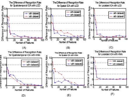
The face recognition rates with respect to different numbers of features for different approaches are shown in Figure 11. The highest values are listed in the Table 1. The results show that spatiotemporal ICA outperforms any other approaches. This gracefully conforms to our expectation. In addition, all approaches perform better using dataset 1 than using dataset 2. This is not surprising since dataset 1 represents more stable condition. What worth noticing at this point are the disparities of performances between using different datasets within the same approach. Even though in Figure 11 (D) we see two performance curves apart in the middle part of the figure, they tend to converge at the end. Especially in Figure 11 (A) two curves get very close. For the other methods the two performance curves are consistently separated. This observation proofs that spatiotemporal ICA is less affected by variations of face expression and other factors. That is spatiotemporal ICA should be more robust than other methods. These findings justify the promise of spatiotemporal ICA for face recognition.

Table 1 The highest recognition rate for each experiment

Spatial ICA Spatiotemporal ICA Localized ICA Euclidean

Classifier

Dataset 1 Dataset 2 Dataset 1 Dataset 2 Dataset 1 Dataset 2 Dataset 1 Dataset 2

LDC 0.6823 0.6212 0.9724 0.9615 0.7616 0.7043 0.4016 0.3143 Highest

Correct

Rate _{K-NN 0.7002 0.6389 0.8954 0.7979 0.7530 0.7028 0.4021 0.3087}

The recognition rate of spatial ICA itself is not good. But after the features were localized the performance was apparently improved (see Figure 11 (B), (C), (E) and (F)). So localization of face images before conducting ICA is a choice for improvement. It is worth for further investigation.

the Euclidean distance features with ICA features. Figure 12 displays the changes of recognition rates after Euclidean distance features have been added to ICA feature spaces. It seems that when the size of ICA feature space is small, Euclidean distance features put great weight for the performance improvement. But when the number of ICA features gets large the weight of Euclidean features in the total feature space dies away dramatically. This means Euclidean features only helps when the ICA performance is not good enough.

0 50 100 150 200 250

0.4 0.5 0.6 0.7 0.8

Number of Features

R e c o g n it io n R a te

Spatial ICA (with K-NN as classifier)

with dataset2 with dataset2 with dataset1 with dataset1 0 50 100 150 200 250

0 0.2 0.4 0.6 0.8 1

Number of ures

R e c o g n it io n R a te

Spatiotemporal ICA (with LCD as classifier)

with dataset2 with dataset2

with dataset1 with dataset1

0 50 100 150 200 250

0 0.2 0.4 0.6 0.8

Number of Features

Re c o g n it io n Ra te

Spatial ICA (with LCD as classifier)

with dataset1 with dataset1 with dataset2 with dataset2

0 50 100 150 200 250 0.2

0.4 0.6 0.8 1

Number of atures

Re c o g n it io n Ra te

Spatiotemporal ICA (with K-NN as classifier)

with dataset2 with dataset2 with dataset1 with dataset1

0 50 100 150 200

0 0.2 0.4 0.6 0.8

Number of Features

R e c o gn it io n R a te

Localized ICA (with LCD as classifier)

with dataset2 with dataset2 with dataset1 with dataset1

0 50 100 150 200

0 0.2 0.4 0.6 0.8

Number of Features

R e c ognit ion R a te

Localized ICA (with KNN as classifier)

with dataset1 with dataset1 with dataset2 with dataset2 Feat

(A) (B) (C)

Fe

(D) (E) (F)

0 20 40 60 80 100 -0.1 0 0.1 0.2 0.3 0.4

Number of Features

D if fe ren c e o f R e c o g n it ion R a te

The Difference of Recognition Rate for Localized ICA with KNN

With dataset1 with dataset2

0 20 40 60 80 100 0

0.1 0.2 0.3 0.4

Number of Features

D if ferenc e of R e c o g n it io n R a te

The Difference of Recognition Rate for Localized ICA with LCD

with dataset2 with dataset1

0 20 40 60 80 100

0 0.1 0.2 0.3 0.4

Number of Features

D if fer enc e of R e c o g n it ion R a te

The Difference of Recognition Rate for Spatiotemporal ICA with LCD

with dataset2 with dataset1

0 20 40 60 80 100 0

0.1 0.2 0.3 0.4

Number of Features

D if fe re nc e of R e c o g n it io n R a te

The Difference of Recognition Rate for Spatial ICA with LCD

with dataset1 with dataset2

0 20 40 60 80 100 0

0.05 0.1 0.15 0.2

Number of Features

D if ferenc e o f R e c o g n it ion R a te

The Difference of Recognition Rate for Spatiotemporal ICA with KNN

with dataset1 with dataset2

0 20 40 60 80 100 0

0.05 0.1 0.15 0.2

Number of Features

D if fe renc e o f R e c o g n it io n R a te

The Difference of Recognition Rate for Spatial ICA with KNN

with dataset1 with dataset2 (B) (C) (A) (F) (E) (D)

Figure 12. The Differences of recognition rates between before and after combining Euclidean features

Acknowledgements

We would like to thank Dr. Victor C. Chen of NRL, who has made many suggestions and provided support and advice.

References

[1] W. Zhao, R. Chellappa, P. J. Phillips, and A. Rosenfeld, Face Recognition: A Literature Survey, ACM Computing Surveys, Vol.35, No. 4, 399-458, December, 2003.

[2] Jongsun Kim, Jongmoo Choi, Juneho Yi, and Matthew Turk, Effective Representation Using ICA for Face Recognition Robust to Local Distortion and partial Occlusion, IEEE Transactions on Pattern Analysis and Machine Intelligence, Vol. 27, No. 12, 2005, 1977-1981.

[3] M. Turk, A. Pentland, Eigenfaces for Recognition, Journal of Cognitive Neuroscience 3(1), 71-86, 1991.

[4] R. Brunell and T. Poggio, Face Recognition: Features vs. Templates, IEEE Trans. Pattern Analysis and Machine Intelligence, 15(10):1042-1053, 1993.

[5] Chengjun Liu and Harry Wechsler, Comparative Assessment of Independent Component Analysis (ICA) for Face Recognition, In: the 2nd International Conference on Audio- and Video-Based Biometric Person Authentication, AVBPA’99, Washington D.C. USA, March 22-24,1999.

[7] Victor C. Chen, “Spatial and Temporal Independent Component Analysis of Micro-Doppler Features” In: 2005 IEEE International Radar Conference Record, 348 – 353, 9 – 12 May 2005, Arlington, VA, USA.

[8] Umbaugh, Scott E. Computer Imaging: Digital Image Analysis and Processing. New York, Taylor & Francis,2005.

[9] Bruce A. Draper, Kyungim Baek, Marian S. Bartlett, and J. Ross Beveridge, Recognizing Faces with PCA and ICA, http://www.face-rec.org/algorithms/Comparisons/draper_cviu.pdf

[10] Andreas Jung, An Introduction to a New Data Analysis Tool: Independent Component Analysis,

http://andreas.welcomes-you.com/research/paper/Jung_Intro_ICA_2002.pdf.

[11] FastICA MATLAB package: http://www.cis.hut.fi/projects/ica/fastica

[12] James V. Stone, Independent Component Analysis: A Tutorial Introduction, Bradford Book, 2004.