Multiobjective multicast routing with Ant Colony Optimization

with Ant Colony Optimization

Polytechnical School, National University of Asunción P.O. Box CC 2111 - Paraguay

{dpinto,bbaran}@pol.una.py http://www.fpuna.edu.py/

Abstract. This work presents a multiobjective algorithm for multicast traffic engineering. The proposed algorithm is a new version of MultiObjective Ant Colony System (MOACS), based on Ant Colony Optimization (ACO). The proposed MOACS simultaneously optimizes the maximum link utilization, the cost of the multicast tree, the averages delay and the maximum end-to-end delay. In this way, a set of optimal solutions, known as Pareto set is calculated in only one run of the algorithm, without a priori restrictions. Experimental results obtained with the proposed MOACS were compared to a recently published Multiobjective Multicast Algorithm (MMA), showing a promising performance advantage for multicast traffic engineering.

1

Introduction

Multicast consists of simultaneous data transmission from a source node to a subset of destination nodes in a computer network [1]. Multicast routing algorithms have recently received great attention due to the increased use of recent point-to-multipoint applications, such as radio and TV transmission, on-demand video, teleconferences and so on. Such applications generally require optimization of

several quality-of service (QoS) parameters such as maximum end-to-end delay and

minimum use of bandwidth resources in a context of traffic engineering.

When a dynamic multicast problem considers several traffic requests, not only

QoS parameters must be considered, but also load balancing and network resources

presents a new MultiObjective Ant Optimization System (MOACS) [4], which finds a set of optimal solutions by simultaneously minimizing the maximum link utilization, the cost of the tree, the maximum end-to-end delay and the average delay. In this way, a whole Pareto set of optimal solutions can be obtained in only one run of the proposed algorithm.

The remainder of this paper is organized as follows. Section 2 describes related works. A general definition of an Optimization Multiobjective Problem is presented in Section 3. The problem formulation and the objective functions are given in Section 4. The proposed algorithm is explained in Section 5 while a brief description of MMA algorithm is given in Section 6. The experimental environment is shown in Section 7 and experimental results are present in Section 8. Finally, conclusions and future works are presented in Section 9.

2

Related work

Several algorithms based on ACO consider multicast routing as a mono-objective problem, minimizing the cost of the tree under multiple constrains. In [5] Liu and Wu proposed the construction of a multicast tree, where only the cost of the tree is minimized using degree constrains. On the other hand, Gu et al. considered multiple parameters of QoS as constrains, minimizing just the cost of the tree [6]. It can be clearly noticed that previous algorithms treated the Traffic Engineering Multicast problem as a mono-objective problem with several constrains. The main

disadvantage of this approach is the necessity of an a priori predefined upper bound

that can exclude good trees from the final solution. In [3], Donoso et al. proposed a multi-tree traffic-engineering scheme using multiple trees for each multicast group.

They took into account four metrics: (i) maximum link utilization α, (ii) hop count,

(iii) bandwidth consumption and (iv) total end-to-end delay. The method minimizes a weighted sum function composed of the above four metrics. Considering the problem is NP-hard, the authors proposed a heuristic algorithm consisting of two steps: (1) obtaining a modified graph, where all possible paths between the source node and every destination node are looked for, and (2) finding out the trees based on the distance values and the available capacity of the paths, in the modified graph. Crichigno and Barán [7] have proposed a Multiobjective Multicast Algorithm (MMA), based on the Strength Pareto Evolutionary Algorithm (SPEA) [8], which simultaneously optimizes the maximum link utilization, the cost of the tree, the maximum end-to-end delay and the average delay. This MMA algorithm finds a set of optimal solutions, which is calculated in only one run, without a priori

3

Multiobjective Optimization Problem

A general Multiobjective Optimization Problem (MOP) [9] includes a set of n

decision variables, k objective functions, and m restrictions. Objective functions and

restrictions are functions of decision variables. This can be expressed as:

Optimize y = f(x) = (f1(x), f2(x) ..., fk(x)).

Subject to e(x) = (e1(x), e2(x), ... ,em(x))≥0,

where x = (x1, x2, ..., xn) ∈ X is the decision vector,

and y = (y1, y2, ... , yk) ∈Y is the objective vector.

(1)

X denotes the decision space while the objective space is denoted by Y. Depending

on the kind of the problem, “optimize” could mean minimize or maximize. The set of

restrictions e(x)≥0 determines the set of feasible solutions Xf ⊆ X and its

corresponding set of objective vectors Yf ⊆ Y. The problem consists in finding x that

optimizes f(x). In general, there is no unique “best” solution but a set of solutions,

none of which can be considered better than the others when all objectives are considered at the same time. This derives from the fact that there can be conflicting objectives. Thus, a new concept of optimality should be established for MOPs.

Given two decision vectors u, v ∈Xf:

f(u) = f(v) iff: ∀i∈{1,2,...,k}: fi(u) = fi(v) f(u) ≤ f(v) iff: ∀i∈{1,2,...,k}: fi(u) ≤ fi(v) f(u) < f(v) iff: f(u) ≤ f(v) ∧ f(u) ≠ f(v)

(2)

Then, in a minimization context, u and v comply with one and only one of the

following three possible conditions:

u ≻v (u dominates v), iff: f(u)<f(v)

v ≻u (v dominates u), iff: f(v)<f(u)

u ~ v (u and v are non-comparable), iff: f(u)≮f(v)∧f(v)≮f(u)

(3)

Alternatively, for the rest of this work, u⊲v will denote that u≻v or u~v. A decision

vector x∈Xfis non-dominated with respect to a set Q⊆Xfiff: x⊲v, ∀v∈Q. When x is

non-dominated with respect to the whole set Xf, it is called an optimal Pareto

solution; therefore, the Optimal Pareto set Xtruemay be formally defined as:

Xtrue={x∈Xf| x is non-dominated with respect to Xf} (4)

The corresponding set of objective vectors Ytrue=f(Xtrue) constitutes the Optimal

Pareto Front.

4 Problem Formulations

For this work, a network is modeled as a direct graph G= (V, E), where V is the set of

nodes and E is the set of links. Let:

cij ∈ ℜ+ : cost of link (i,j).

dij ∈ ℜ+ : delay of link (i,j), in ms.

zij ∈ ℜ+ : capacity of link (i,j), in Mbps.

tij ∈ ℜ+ : current traffic of link (i,j), in Mbps.

φ ∈ ℜ+ : traffic demand, in Mbps.

s ∈ V : source node of a multicast group.

Nr⊆ V-{s}: set of destinations of a multicast group.

T : multicast tree with source in s and set of destinations Nr.

Also, let p(s,n)⊆T be the path that connects the source node s with a destination node

n∈Nr. Finally, let dp(s,n) represent the delay of the path p(s,n), given by the sum of the

link delays that conform the path, i.e.:

d

=

∑

i , j∈ps , n

d

Using the above definitions, a multicast routing problem for Traffic Engineering

may be stated as a MOP that tries to find the multicast tree T that simultaneously

minimizes the following objective functions: 1- Maximum link utilization of the tree:

α

=

Max

i , j∈T

{

α

}

where

α

=

φ



t

/

z

2- Cost of the multicast tree:

C

=

φ

∗

∑

i , j∈T

c

3- Maximum end-to-end delay of the multicast tree:

d

¿

¿

D

=

Max

n∈N_r

¿

¿

(8)

4- Average delay of the multicast tree:

D

=

∣Nr∣

∗

∑

n∈N_r

d

where |Nr| denotes the cardinality of Nr.

The problem is subject to a link capacity constraint:

α

≤1

A simple example follows to clarify the above notation.

Example 1. Given the NSF network topology of Fig. 1 [7], the number over each link

(i,j) denotes dijin ms, cij, and tijat a given time (in Mbps). NSF network consist of 14

=0.2 Mbps, s=5, and Nr= {0, 2, 6, 13}. Fig. 1 shows a multicast tree (T) while Table 1

presents the objective functions calculated for this tree.

Fig. 1. The NSF Net. αm=0.73; C=6.4; Dm=23; Da=16.5.

Table 1. Objective Functions Calculated for Example 1.

Tree

(i,j) (5,4) (4,2) (2,0) (5,6) (6,9) (9,13)

dij 7 7 9 7 7 8

cij 6 4 2 1 10 9

tij 0.1 0.1 0.9 0.6 0.7 0.8

zij 1.5 1.5 1.5 1.5 1.5 1.5

αij 0.2 0.2 0.73 0.53 0.6 0.53

Delay paths

dp(5,2) d5,4+ d4,2 =7+7= 14

dp(5,0) d5,4+d4,2+d2,0=7+7+9= 23

dp(5,6) d5,6 = 7

dp(5,13) d5,6+d6,9+d9,13=7+7+8= 22

Metrics of the solution Tree

αm α2,0 = 0.73

C φ*(c5,4 + c4,2 + c2,0 + c5,6 + c6,9 + c9,13) = 0.2*(6+4+2+1+10+9) =

6.4

Dm dp(5,0) = 23

Da (dp(5,2)+ dp(5,0)+ dp(5,6)+ dp(5,13)) / |Nr| = (14+23+7+22) / 4 = 16.5

For the same example, Figure 2 presents in (a), (b) and (c) three different alternative solutions, for the same multicast group, to clarify the concept of non-dominance. Notice that each tree is better than any other in at least one objective.

through a linear combination (as weighted sum) nor are any of them treated as a restriction. This way, using the concept of dominance, a whole set of optimal Pareto solutions is calculated.

Table 2. “Optimal Pareto Set” and “Optimal Pareto Front” for Example 1.

Optimal Pareto Set (Trees)

Optimal Pareto Front (Objective Vectors)

αm C Dm Da

S1 (5,6),(5,4),(4,2),(4,10),(2,0),(10,12),(12,13) 0.73 5 20 36

S2 (5,6),(5,4),(6,1),(6,9),(4,2),(1,0),(9,8),(8,12),(12,13) 0.6 8.6 21.75 36

S3 (5,6),(5,4),(6,1),(6,9),(4,2),(1,0),(9,13) 0.67 7.6 19.75 36

S4 (5,6),(5,4),(6,9),(4,2),(9,13),(2,0) 0.73 6.4 16.50 23

S5 (5,6),(5,4),(6,1),(4,2),(4,10),(1,0),(10,12),(12,13) 0.73 4 26.75 63

S6 (5,6),(5,4),(6,1),(4,2),(4,10),(1,0),(10,12),(12,13) 0.6 6.2 23.25 36

S7 (5,6),(6,1),(1,0),(0,3),(0,2),(3,10),(10,12),(12,13) 0.73 3.6 41 76

S8 (5,6),(5,4),(6,1),(4,2),(1,0),(2,7),(7,13) 0.53 7 23.75 38

S9 (5,6),(5,4),(4,2),(4,10),(10,12),(10,3),(12,13),(3,0) 0.6 5.2 24.25 4

S10 (5,6),(5,4),(4,10),(10,3),(10,12),(3,0),(12,13),(0,2) 0.73 4.8 33 49

(b)

(c)

Fig. 2. The NSF Net. (a) to (c) show different Pareto solutions for the same multicast group of example 1.

For the presented example, the set of optimal Pareto set and corresponding objective functions are shown in Table 2. Notice that solution S1 corresponds to

Figure 2(a), S2 corresponds to Figure 2(b) and S3 corresponds to Figure 3(c).

5

Ant Colony Optimization Approach

Ant Colony Optimization (ACO) is a metaheuristic inspired by the behavior of natural ant colonies [10]. In the last few years, ACO has received increased attention by the scientific community as can be seen by the growing number of publications and different application fields [4]. Even though, there are several ACO variants that can be considered, a standard approach is next presented [11].

5.1 Standard Approach

ACO uses a pheromone matrix τ = {τij} for the construction of potential good

solutions. The initial values of τare set as τij= τ0∀(i, j), where τ0 > 0. It also takes

advantage of heuristic information (known as visibility) using ηij= 1/dij. Parameters

α and β define the relative influence between the heuristic information and the

pheromone levels [10]. While visiting node i, Nirepresents the set of neighbor nodes

that are not yet visited. The probability (pij) of choosing a next node j, while visiting

node i, is defined by equation (11). At every iteration of the algorithm, each ant of a

colony constructs a complete solution T using (11), starting at source node s. Pheromone evaporation is applied for all (i, j) of τ, according to τij= (1 - ρ) •τij, where

parameter ρ∈(0;1] determines the evaporation rate. Considering an elitist strategy,

the best solution found so far Tbest updates τaccording to τij= τij+∆τ, where ∆τ=

1/l(Tbest) if (i, j) ∈ Tbestand ∆τ= 0 otherwise. Where l(Tbest) represents and objective

τ_ijα

¿

∑

τ_igα

¿

if j

∈

N

0

otherwise

¿

p

=

¿

{

¿ ¿ ¿

¿

(11)

5.2 Proposed Algorithm

Following the MultiObjective Ant Colony Optimization Algorithm (MOACS) scheme

[4], which is a generalization of the ACS [10], the proposed algorithm uses a colony

of ants (or agents) for the construction of m solutions T at every generation. Then, a

known Pareto Front Yknow [9] is updated including the best non-dominate solutions

that have been calculated so far. Finally, the gathered information is saved updating a pheromone matrix τij. Fig. 3 (a) presents the general procedure of MOACS. In

general, if the state of Yknowwas changed, the pheromone matrix τijis re-initialized

(τij= τ0 ∀(i,j)∈V) to improve exploration in the decision space Xf. Otherwise, τij

is globally updated using the solutions of Yknow to exploit the knowledge of the best

known solutions. Note that only the links of found solutions T in Yknow are used to

update the pheromone matrix τij. To construct a solution, an ant begins its job in the

source node s. A non-visited node is pseudo-randomly [4] selected at each step. This

process continues until all destination nodes of the multicast group are reached.

Considering R as the list of starting nodes, Kias the list of feasible neighboring nodes

to the node i, Dras the set of destination nodes already reached, the procedure to find

a solution T is summarized in Fig. 3 (b).

Begin MOACS

read G, (s,Nr), φ and tij initialize τij with τ0

while (stops criterion is not verified)

repeat (m times)

T=Build Solution

if (T {T⊀ y|Ty∈Yknow}) then

Yknow=Yknow∪T-{Tz|T T≻ z} ∀Tz∈Yknow end if

end repeat

if (Yknow was changed) then

Initialize τij with τ0 else

repeat (for every T∈Yknow)

τij=(1-ρ).τij+ρ.∆τ ∀(i,j) ∈T end repeat

end while return Yknow

end MOACS

(a)

Begin Build Solution

T = {∅}; Dr = {∅}; R = R ∪ s repeat (until R = {∅} or Dr = Nr)

select node i of R and build set Ki if (Ki = {∅}) then

R = R – i /*erase node without feasible neighbor*/ else

select node j of Ki /*pseudo-random rule*/ T = T ∪ (i,j) /*constructions of tree T*/

R = R ∪ j /*constructions list of starting nodes*/ if (j ∈ Nr) then

Dr = Dr∪ j /*node j is node destination*/ end if

τij=(1-ρ).τij+ρ.τ0 /*update pheromone*/ end if

end repeat

Prune Tree T /*eliminate nor used links*/ return T /*return solution*/ end Build Solution

(b)

Fig. 3. (a) General Procedure of MOACS and (b) Procedure to Build Solution.

where:

Δτ

=

1

∑

∀T∈Y

know



α

∗

C

∗

D

∗

D



and ρ ∈ (0, 1] represents trail persistence.

6

Multiobjective Multicast Algorithm

Multiobjective Multicast Algorithm (MMA), recently proposed in [7], is based on the

Strength Pareto Evolutionary Algorithm (SPEA) [8]. MMA holds an evolutionary population P and an external Pareto solution set Pnd. Starting with a random

population P of solutions, the individuals evolve to Pareto optimal solutions to be

included in Pnd. The pseudo-code of the main MMA algorithm is shown in Fig. 4(a),

while its codification is represented in Fig. 4(b).

Begin MMA

Read G, (s,Nr), φ and tij

Initialize P

Do {

Discard individuals Evaluate individuals

Update non-dominated set Pnd

Compute fitness Selection

Crossover and Mutation

} while stop criterion is not verified

endMMA

(a)

(b)

Fig. 4. (a) Pseudo-code of main MMA algorithm (b) Relationship between a chromosome, genes and routing tables for a tree with s=0 and Nr={2, 3}.

The MMA algorithm begins reading the variables of the problem and basically proceeds as follows (see pseudo-code in Fig. 4(a)):

Build routing tables: For each ni∈ Nr, a routing table is built. It consists of the ψ

shortest and ψ cheapest paths. ψ is a parameter of the algorithm. A chromosome is

represented by a string of length |Nr| in which each element (gene) gi represents a

path between s and ni. See Fig. 4(b) to see a chromosome that represents the tree in

Fig. 4(b).

Discard individuals: In P, there may be duplicated chromosomes. Thus, new randomly generated individuals replace duplicated chromosomes.

Evaluate individuals: The individuals of P are evaluated using the objective

functions. Then, non-dominated individuals of P are compared with the individuals

in Pnd to update the non-dominated set, removing from Pnd dominated individuals.

Compute fitness: Fitness is computed for each individual, using SPEA procedure [8].

Selection: Traditional tournament or roulette methods may be used [8]. In this works,

a roulette selection operator is applied over the set Pnd ∪ P to generate the next

Crossover and Mutation: MMA uses two-point crossover operator over selected pair of individuals. Then, some genes in each chromosome of the new population are randomly changed (mutated), obtaining a new solution. The process continues until a stop criterion, as a maximum number of generations, is satisfied.

7 Experimental Environments

MOACS and MMA have been implemented on a 350 MHz AMD Athlon computer with a 128 MB of RAM. The compiler used was Borland C++ V 5.02.

In order to evaluate the proposed MOACS approach to a recently published algorithm as MMA [7], several test problems were used, but only two will be presented. Each test was divided into four sub-tests (or scenarios) where the networks are under different load level:

• low (0 ≤ αij ≤ 0.4),

• medium (0.4 ≤ αij ≤ 0.7),

• high (0.7 ≤ αij ≤ 0.9), and

• saturation (0.9 ≤ αij ≤ 1).

MMA parameters were: 40 chromosomes and mutation probability of 0.3, suggested in [7], while MOACS parameters were: 40 ant, 0.95 pseudo-random probability, 0.95 trail persistence. The runs stopped after 2000 generations.

For each sub-test an approximation of the Pareto Front corresponding to each multicast group is obtained using a procedure with the following three steps:

1) Each algorithm (MOACS & MMA) was run ten times to calculate average

values.

2) A set solutions “Y” conformed by all solutions of both algorithms was calculated.

3) The dominated solutions were eliminated from “Y”, and an approximation of

“Ytrue” was created.

7.1 Test Problem 1

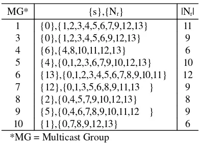
The first test problem was the NSF network of Example 1, with ten multicast groups (MG) shown in Table 3.

The number of optimal solutions of the approximated Pareto Front Ytrue is

presented in Table 4, for each multicast group and load level.

Table 3. Multicast Groups for Test Problem 1.

MG* {s},{Nr} |Nr|

1 {0},{1,2,3,4,5,6,7,9,12,13} 11

MG* {s},{Nr} |Nr|

1 {0},{1,2,3,4,5,6,7,9,12,13} 11

3 {0},{1,2,3,4,5,6,9,12,13} 9

4 {6},{4,8,10,11,12,13} 6

5 {4},{0,1,2,3,6,7,9,10,12,13} 10

6 {13},{0,1,2,3,4,5,6,7,8,9,10,11} 12

7 {12},{0,1,3,5,6,8,9,11,13 } 9

8 {2},{0,4,5,7,9,10,12,13} 8

9 {5},{0,4,6,7,8,9,10,11,12 } 9

10 {1},{0,7,8,9,12,13} 6

*MG = Multicast Group

Table 4. Number of Optimal Solutions in Ytrue for each MG and load level for Test Problem 1.

MG

|Ytrue|

Lo w

Hal f

Hig h

Saturatio n

1 62 51 62 26

2 33 21 32 23

3 19 25 25 13

4 11 14 10 10

5 20 15 9 17

6 45 29 31 18

7 20 19 13 13

8 14 16 14 5

9 18 16 19 15

10 11 9 13 7

7.2 Test Problem 2

The second test was carried out using the NTT network topology [7] of Fig. 5, where

a delay dij over each link (i,j) is shown. NTT network consists of 55 nodes and 144

links.

Multicast groups used in this test are shown in Table 5 and the number of optimal

Fig. 5. NTT network used in test problem 2. Numbers over links represent propagation delay in ms.

Table 5. Multicast Groups for Test Problem 2.

MG {s},{Nr}

| N

r|

1 {51},{0,3,4,8,13,15,16,22,30,31,40,41,44,47,50,54} 1

6

2 {48},{2,3,5,6,7,8,9,10,11,12,14,15,16,20,24,25,28,29,30,31,33,34,40,43,4

4,46,49,50,51,52,54}

3 1

3 {46},{0,3,5,6,7,12,14,15,16,17,20,23,24,26,28,29,31,32,34,35,37,39,47,48

,50}

2 5

4

{26},{0,1,2,3,4,5,6,7,8,9,10,11,12,13,14,15,16,17,18,19,20,22,23,24,25,27, 28,29,30,31,32,3334,35,36,37,38,39,40,41,42,43,44,45,46,47,49,50,51,52 ,53,54}

5 2

5 {36},{1,7,8,12,14,16,18,20,21,25,26,28,30,32,33,34,35,37,39,41,43,44,45,

46,48,49,50,51,52,53,54}

3 1

6 {30},{0,5,10,12,15,25,29,31,36,42,44,46} 1

2

7 {13},{4,6,10,11,14,17,18,19,23,28,30,34,37,38,42,44,53} 1

7

8 {21},{0,1,3,4,5,6,7,8,9,10,11,12,13,14,15,17,18,19,20,22,23,24,25,26,27,28

9 {51},{1,3,7,11,15,16,17,18,26,27,30,37,42,43,46,50,52} 1 7

10 {11},{1,4,5,6,9,10,12,15,16,17,19,20,22,23,27,29,30,31,32,34,35,36,37,38,

39,40,42,43,45,4647,48,49,50,51,52,54}

3 7

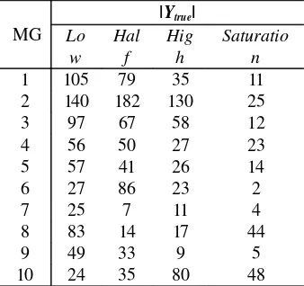
Table 6. Numbers of Optimal Solutions Ytrue for each MG and load level, for Test Problem 2.

MG

|Ytrue|

Lo w

Hal f

Hig h

Saturatio n

1 105 79 35 11

2 140 182 130 25

3 97 67 58 12

4 56 50 27 23

5 57 41 26 14

6 27 86 23 2

7 25 7 11 4

8 83 14 17 44

9 49 33 9 5

10 24 35 80 48

8

Experimental Results

Next, the experimental results for each test problem and different load levels are presented separately, comparing the results using the proposed MOACS to the corresponding results using MMA.

8.1 Test Problem 1

In these tests using the NSF network with 14 nodes and 42 links, it can be easily seen that in general MOACS outperforms MMA finding a larger number of Pareto solutions (see averages in Table 7). Only in column “Average for each MG” for multicast groups 4 (42 %) and 9 (49.25%) MMA may seem better than MOACS, but in the rest of the tests, MOACS is widely superior.

Table 7. Comparison of solutions in Ytrue for each MG and load level, for Test

Problem 1.

MG Low Medium High Saturation

Average for each MG

MOACS MMA MOACS MMA MOACS MMA MOACS MMA MOACS MMA

1 80 % 1 % 96 % 0 % 86 % 0 % 100 % 0 % 90.50 % 0.25%

3 95 % 1 % 96 % 0 % 88 % 2 % 94 % 0 % 93.25 % 0.75%

4 36 % 41 % 21 % 43 % 10 % 34 % 50 % 50 % 29.25 % 42%

5 82 % 2 % 87 % 1 % 68 % 7 % 58 % 29 % 73.75 % 9.75%

6 76 % 0 % 59 % 2 % 87 % 0 % 91 % 0 % 78.25 % 0.50%

7 20 % 28 % 40 % 22 % 15 % 32 % 100 % 0 % 43.75 % 20.50%

8 100 % 0 % 91 % 4 % 93 % 1 % 100 % 0 % 96 % 1.25%

9 28 % 37 % 12 % 76 % 16 % 51 % 65 % 33 % 30.25 % 49.25%

10 55 % 19 % 89 % 11 % 77 % 16 % 57 % 43 % 69.50 % 22.25%

Average for each Load Level Global Average

60% 16% 62% 18% 54% 19% 82% 15% 64.4% 17.1%

8.2 Test Problem 2

In this seconds test, MOACS again demonstrates the best performance (see averages

in Table 8). See in Table 8 column “Average for each MG”, that only for multicast

group 5 (15 %) MMA is superior. Also notice that in the “Global Average” MOACS

calculated 40 % of Ytrue solutions while MMA only found 3 %. Even more,

considering “Global Average,” MOACS achieved 67.2 % of Ytrue solutions while

MMA only reached 17.1 %.

Table 8. Comparison of Solutions with Ytrue for each Multicast group and level load

for test problem 2

MG Low Medium High Saturation

Average for each MG

MOACS MMA MOACS MMA MOACS MMA MOACS MMA MOACS MMA

1 42 % 5 % 46 % 1 % 59 % 5 % 89 % 0 % 59 % 3 %

2 10 % 3 % 10 % 0 % 11 % 0 % 58 % 0 % 22 % 1 %

3 27 % 0 % 25 % 0 % 27 % 0 % 65 % 0 % 36 % 0 %

4 9 % 1 % 8 % 2 % 10 % 1 % 68 % 0 % 24 % 1 %

5 7 % 6 % 2 % 14 % 3 % 7 % 4 % 34 % 4 % 15 %

6 96 % 0 % 64 % 0 % 86 % 0 % 100 % 0 % 87 % 0 %

7 70 % 1 % 36 % 7 % 60 % 1 % 75 % 25 % 60 % 9 %

8 10 % 0 % 10 % 1 % 8 % 2 % 40 % 0 % 17 % 1 %

9 64 % 0 % 85 % 0 % 42 % 7 % 100 % 0 % 73 % 2 %

10 10 % 0 % 10 % 0 % 9 % 1 % 52 % 0 % 20 % 0 %

Average for Load Level Global Average

35 % 2 % 30 % 3 % 32 % 2 % 65 % 6 % 40 % 3 %

It can be concluded from Tables 7 and 8 that MOACS outperforms MMA for this type of MOP, finding a larger number of Pareto solutions.

From these experimental results, the following conjecture can be stated. ACO algorithms as MOACS build relatively good solutions using heuristic information (visibility) and avoiding not feasible solutions; therefore, in general, ACO algorithms

are better suited for constructing good solution, compared to Multiobjective

are probabilistic; thus, MMA may eventually outperform MOACS, as shown in Table

8 (row 5 and column Average for each MG).

9

Conclusions

This paper introduces a new approach based on MOACS to solve the multicast routing problem. The proposed MOACS is able to optimize simultaneously four objective functions, such as, (1) maximum link utilization (αm), (2) cost of the

routing tree (C), (3) maximum end-to-end delay (Dm) and (4) average delay (Da). This

new proposal is able to solve a multicast routing problem in a truly multiobjective context, considering all four objectives at the same time, for the first time using an algorithm based on Ant Colony Optimization. The new approach calculates not only one possible solution, but a whole set of optimal Pareto solutions in only one run. This last feature is especially important since the most adequate solution can be chosen for each particular case without a priori restrictions that may eliminate otherwise good solutions. To validate the new approach, MOACS was compared to the MMA, a representative algorithm for solving the multicast routing problem in a truly multiobjective context, for Traffic Engineering. The experimental results showed that MOACS is able to find a larger number of Pareto solutions than MMA for different network topologies, different load level and various multicast groups, i.e.

MOACS found better solutions in average than MMA.

As a future work, the authors will perform more tests over other network topologies and other metrics will be also considered to make sure that algorithms based on Ant Colonies are a promising approach for traffic engineering. At the same time, authors consider the study of convergence time for the proposed algorithm, as well as the control traffic load it causes.

References

1. A. Tanenbaum, Computer Networks, Prentice Hall 4º Edition, 2003.

2. Y. Seok, Y. Lee, Y. Choi, and C. Kim, “Explicit multicast routing algorithm for

constrained traffic engineering”, IEEE 7th International Symposium on Computer

and Communications (ISCC’02). Italy, 2002.

3. Y. Donoso, R. Fabregat, and J. Marzo, “Multiobjective optimization algorithm for

multicast routing with traffic engineering”, IEEE 3rd_{International Conference on}

Networking (ICN’2004), Guadalupe, French Caribbean, March – 2004.

4. M. Schaerer, and B. Barán. “A Multiobjective Ant Colony System For Vehicle

Routing Problem With Time Windows”, IASTED International Conference on

Applied Informatics, Innsbruck, Austria, 2003.

5. Y. Liu, and J. Wu. “The degree-constrained multicasting algorithm using ant

6. J. Gu, C. Chu, X. Hou, and Q. Gu. “A heuristic ant algorithm for solving QoS multicast routing problem” Evolutionary Computation, 2002. CEC '02. Volume 2, pp 1630-1635.

7. J. Crichigno, and B. Barán. “Multi-objective Multicast Routing Algorithm for Traffic Engineering” ICCCN’2004, California, USA, 2004.

8. E. Zitzler, and L. Thiele, “Multiobjective Evolutionary Algorithms: A comparative Case Study and the Strength Pareto Approach”, IEEE Trans. Evolutionary Computation, Volume 3, No. 4, 1999, pp 257-271.

9. D. A. Van Veldhuizen. “Multiobjective Evolutionary Algorithms: Classifications, Analysis, and New Innovations”, Ph.D Thesis, Graduated School of Engineering of the Air Force Institute of Technology, Air University, 1999.

10. M. Dorigo, and L. M. Gambardella. “Ant Colony System: A cooperative learning approach to the traveling salesman problem” IEEE Transactions on Evolutionary Computation, 1: 1, pp 53-66, 1997.

11. M. Guntsch and M. Middendorf. “A Population Based Approach for ACO”. In

Stefano Cagnoni, Jens Gottlieb, Emma Hart, Martin Middendorf, and Günther

Raidl, Applications of Evolutionary Computing, Proceedings of