Evolutionary optimization in dynamic fitness landscape environments

EVOLUTIONARY OPTIMIZATION IN DYNAMIC FITNESS LANDSCAPE ENVIRONMENTS

Aragón V. S., Esquivel S. C.,

Laboratorio de Investigación y Desarrollo en Inteligencia Computacional (LIDIC) 1 Facultad de Ciencias Físico, Matemática y Naturales

Universidad Nacional de San Luis Ejército de los Andes 950 – Local 106

5700 – San Luis Argentina. {vsaragon, esquivel}@unsl.edu.ar

ABSTRACT

Non-stationary, or dynamic, problems change over time. There exist a variety of forms of dynamism. The concept of dynamic environments in the context of this paper means that the fitness landscape changes during the run of an evolutionary algorithm.

Genetic diversity is crucial to provide the necessary adaptability of the algorithm to unexpected changes.

Two key concepts to maintain genetic diversity in the population are incorporated to the algorithm and proposed here: macromutation operators and random immigrants.

The algorithm was tested on a set of dynamic testing functions provided by a dynamic fitness problem generator. The main goal was to determine the algorithm ability to face changes and dimensional or multimodal scalability in the functions.

The effectiveness and limitations of the proposed algorithm in diverse scenarios of a dynamic environment is discussed from results empirically obtained.

Keywords: Evolutionary computation, dynamic fitness landscape, macromutation, random inmigrants, multi-modal optimization.

1

1.

INTRODUCTION

In general the conditions of an optimization problem changes by one of the following reasons or a combination of both [1]: 1) The objective function changes itself, 2) The constraints change. A change in the objective function appears when the purpose of the problem changes. Here conditions which were considered desirable before can turn out to be undesirable now and vice versa. Changes in constraints, which modify feasibility of solutions, are related to resources and their availability. Changes can be small or big, soft or abrupt, chaotic, etc. When changes are big, abrupt or chaotic the similarity between solutions found so far and the new ones can be worthless. Even under these hard environments Evolutionary Computation (EC) offers advantages, which are absent in other heuristics when searching for solutions to non-stationary problems. The main advantage relies in the fact that Evolutionary Algorithms (EAs) keep a population of solutions. Consequently, facing the change, they allow moving from a solution to another one to determine if any of them are of merit to continue the search from them instead of from scratch [2]. Goldberg and Smith [3], Cobb[4] and Grefenstette [5] initiated the research related to the behaviour of EAS on dynamic fitness functions between 1987 and 1992. Recently the interest in this area was dramatically incremented [6], [7], [8], [9], [10], [11], [12], [13], [14], and [15]. The following sections are organized as follows. Section 2 presents a definition of dynamic environments studied in this work. Section 3 describes the dynamic test functions used. Section 4 describes the EA. In section 5 the experiments performed are described. In section 6 results are discussed and finally this document shows our conclusions, current and future work.

2.

DYNAMIC FITNESS PROBLEM DEFINITION

A general definition, which describes and characterizes a dynamic fitness function, is introduced here. The approach we follow assumes that each dynamic function consists of a base static function and a sequence of dynamic functions obtained from the base function and the application of a set of dynamic rules.

Definition 1:

(

( ), ,

)

otherwise ) I ( 0 if ) ( : follows as defined is function fitness dynamic A . time the and vector a space, searching the be Let

1 t t

t t t t t s ch x DF g DF t x fb DF N t x r r r − = = ∈ Ψ ∈ Ψ

where fb0(xr) is the base static function with m possible features to be modified.

Definition 2: Function gt is more precisely defined as follows:

(

DF

1

(

x

),

ch

,

s

)

apply

_

changes

_

on

_

DF

1

(

ch

,

L

)

g

t t−

r

t t

=

t− t

where the first argument of apply_changes_on_DFt-1:

{

}

U U

m i n j j i t FL c ch 1 1 , = = =

is an ordered set of size mxn of all possible changes at time t. When building this set, ciindicates which function characteristic changes and FLj indicates which part of the DFt-1landscape will be modified within the ith characteristic.

The second argument of apply_changes_on_DFt-1, L is a binary vector of length mxn, which depending on st indicates which members of cht are selected and which are not selected to modify

DF.

3.

DYNAMIC TESTING FUNCTIONS

In this section we will see that the functions provided by the Test problem Generator [16] belong to the dynamic functions defined in ( I ).

In this case we have:

The dynamic function DFt defined as in ( I ) with the base static function defined as:

(

)

(

)

_       − + + − ∗ −

= ₌1, 1 ₁ 2 .... 2

)

( _{i k i}t _it t_{i k ni}t

t x x x x R H max x fb r

which specifies a “field of cones”, where k indicates the number of cones in the environment and each cone is independently specified by its location (x1i, x2i, …, xni), its height Hi, and its slope Ri. The components of the vector defining the cone location are xij∈ [-1,1].

Each of these cones is combined together by means of the max function. Each time it is called the generator creates a randomly generated morphology. The user specifies the range of random values for the height, slope and location of cones:

Hi∈ [Hbase, Hbase + Hrange], Ri∈ [Rbase, Rbase + Rrange] and xij∈ [-1,1].

In this case, when building the set cht of all possible changes, a characteristic ci ∈ {height, slope, location} (m = 3) and FLj indicates which of the k cones of the DFt-1landscape will be modified within the ith characteristic. Consequently, when apply_changes_on_DFt-1operates, the corresponding modifications in DF will be done only for those characteristics in the cones where

Lj+k(i-1)= 1, in the binary vector L, for 1 ≤ i ≤ m, 1 ≤ j ≤ k.

In this way we can see that the generator allows changing height, slope and location of one or more cones in the field of cones, which represents the morphology of the fitness landscape.

. time the and vector a space, searching

the x R t N

Rn ∈ n ∈

=

The severity of changes has many degrees, such that degree 1.0 corresponds to soft and/or small changes and degree 4.0 to chaotic changes. The degree of severity is calculated by using the logistic function:

) 1

( ₁

1 −

− ∗ − ∗

=

= _{p p p}

t _{Y A Y Y}

s

where A is a constant indicating the degree of severity of the characteristic (height, slope, or location) that will be modified and Yp is the value of the logistic function at iteration p. For more details see [16].

4.

EVOLUTIONARY ALGORITHM

We chose an evolutionary algorithm which combines and exploit various forms of macro-mutation similar to both, the hyper-mutation and random immigrants initially designed by Grefenstette [5].

4.1. REPRESENTATION

The population P is composed of a constant number N of chromosomes. Each individual consists of a single chromosome, where each gene is a real value in the interval [-1.0,1.0] representing a coordinate in the search space. That is, the ith individual in the population P is represented by the chromosome:

Pi = 〈xi1, xi2, …, xil〉

where xij denotes the jth coordinate of the ith individual with j = 1,…,l and l is the chromosome length.

4.2. OPERATORS

Conventional operators:

Selection: Couples of parents for the mating pool are selected by means of proportional selection.

Recombination: The conventional one point crossover is used to exchange genetic material

between parents. The operator is applied with a Pcrossprobability.

Mutation: Uniform mutation is used and it is applied with a Pmutprobability. When an individual

undergoes mutation, each gene has exactly the same chance of undergoing mutation. As a result the mutated gene has a new allele value randomly chosen from the domain of the corresponding parameter (vector component).

Specialized operators for macromutation:

Recrudescence: This operator increments the probabilities of undergoing recombination and/or

mutation for a part of the population. It is applied in every generation with a probability Precru and produces a radical genotypic reorganization on the individuals where it is applied. These individuals are selected randomly with uniform probability.

Crisis: Acts as the recrudescence operator but it is applied on the whole population at determined

Random immigrants: A percentage z% of the population is replaced by individuals randomly generated.

4.3. EVOLUTIONARY ALGORITHM PSEUDOCODE

The structure of the proposed evolutionary algorithms follows:

0. t = 0 /* initial generation */ 1. Generate fbt function and set DFt = fbt 2. Initialise Pt /* initial population */ 3. Evaluate Pt

4. while (actual_number-changes < = total_number_changes) do 5. {

6. t = t + 1

7. if (crisis) and (t < number_gen_with_crisis) then 8. Apply_crisis_operator

9. Generate next population P’t using traditional operators and recrudecence if appropiate 10. Evaluate P’t

11. Calculate _statistics of P’t

12. Remember_the_best_of_generation /* elitism */ 13. if (function_changes) then

14. {

15. Store_statistical_report 16. Build_vector_L

17. Apply_changes_on_DFt-1(ch, L) and obtain new DFt 18. }

19. if (occured_changes) then 20. { Evaluate P’t with new DFt 21. Calculate _statistics of P’t

22. Remember_the_best_of_generation /* elitism */ 23. Apply_crisis_operator

24. }

25. if (finish_apply_crisis) then 26. {

27. apply_random_inmigrants_operator 28. Evaluate P’t

29. Calculate _statistics of P’t

30. Remember_the_best_of_generation /* elitism */ 31. }

32. Let Pt = P’t

33. } /* end while */ 34. Report_ statistics

If a change must occur we store in the L vector what changes are to be done and in which cones on the landscape to apply them (see line 16). Then the apply_changes function obtains a new dynamic fitness function in line 17.

In the line 22, occured_function tests if a change effectively had occurred, in which case the application of macromutation operators creates the necessary genetic diversity. Then a new generation begins and so on, until the end condition is reached.

5.

EXPERIMENTS DESCRIPTION

5.1. PARAMETERS OF THE EVOLUTIONARY ALGORITHM

The parameter settings for the EA remain fixed throughout all experiments and all scenarios, and were determined as the best after some initial trials:

The population size |P| was set to 100 individuals. Pcross and Pmut were fixed at 0.25 and 0.5, respectively. For recrudescence, Precruwas set to 0.2, and the augmented probabilities of crossover and mutation were fixed at 0.5 and 0.8, respectively. The crisis operator is applied to the 10% of the number of generation, between two consecutive changes in the environment. The percentage of random immigrants was fixed at 30% of the population. Immigrants are inserted when a change was detected and after the application of the crisis operator. This decision prevents that new immigrants be affected by the crisis operator. The individuals to be replaced by immigrants are randomly selected with equal probability. A number of experiments were designed differing in the function selected and the changes to perform on it. For each of these experiments 30 runs were performed with distinct initial population. Values in tables of section 6 are mean values.

5.2. PARAMETERS OF THE FUNCTION GENERATOR

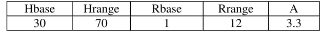
Table 1 shows the parameter settings for the generator for all functions.

Hbase Hrange Rbase Rrange A 30 70 1 12 3.3

The constant A is used by the logistic function to determine the change severity. The value chosen for A creates a severity of degree between median and large (near to the upper limit of 4.0 required by the simulator).

We worked on 5 different functions whose features of dimensionality and multimodality (number of cones) are indicated in table 2.

Function dim-#cones dim-#cones dim-#cones dim-#cones dim-#cones dim-#cones

f1 2-5 2-30 5-5 5-30 10-5 10-30

f2 2-5 2-30 5-5 5-30 10-5 10-30

f3 2-5 2-30 5-5 5-30 10-5 10-30

f4 2-5 2-30 5-5 5-30 10-5 10-30

f5 2-5 2-30 5-5 5-30 10-5 10-30

[image:6.595.135.449.503.536.2]

Table 1. Parameter Settings for the Generator

Because the generator randomly creates the functions, we adopted the following working methodology. For example for function f1 (see table 3), first we select heights (H) and slopes (R) with the greatest multimodality. C indicates the cone identifier.

C H R C H R C H R

1 0.000000 0.000000 11 61.556893 5.811603 21 86.834253 6.018287 2 39.254461 13.425523 12 93.957383 2.548734 22 46.736654 7.188162 3 88.798945 2.201534 13 60.579642 5.152966 23 48.702074 10.149014 4 75.510408 3.834928 14 89.383742 8.525519 24 36.545954 11.617667 5 30.118679 12.300053 15 46.533252 10.423104 25 91.210267 2.415192 6 57.280549 13.325354 16 35.963361 2.647181 26 54.656304 3.071827 7 90.701662 12.850853 17 84.346277 5.990322 27 39.453273 5.902942 8 69.366403 12.017908 18 57.764563 3.513832 28 71.159464 5.190918 9 83.719877 6.973150 19 31.260441 13.380469 29 86.679211 8.862785 10 99.706369 2.875522 20 32.983730 12.417660 30 49.167685 7.235978

A similar table, not shown here for space limitations, is built for the 10 coordinates of each cone (the greatest dimensionality) the data associated with the experiments are available for any interested reader.

When scalability is to be modified, to work with lower dimensions and lesser number of cones we obtain the required values from these tables. For example if we wish to work with f1 for 2-5, the heights and slopes of the first five cones are retrieved from the tables only for the first two dimensions of the tables of coordinates. Analogously we proceeded with the remaining functions.

This working methodology allowed us to study the adaptability of the algorithm to changes and its behaviour when facing scalability in space dimension and number of cones.

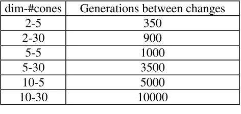
Table 4 shows how, depending on dimensionality and multimodality, the intervals between changes were fixed for all functions, the main goal here was to locate the optimum with an acceptable error.

dim-#cones Generations between changes

2-5 350 2-30 900

5-5 1000 5-30 3500 10-5 5000 10-30 10000

[image:7.595.180.416.539.651.2]

Each time the algorithm run as many generations as changes were desired to make. For all experiments we fixed at 4 the number of changes. For example, for each of the functions with dimensionalty-multimodality equal to 2-5 a total of 1400 generations were needed.

Table 3. Initial Heights and Slopes for f1b0

5.3. TYPES OF CHANGE

Four scenarios were designed, each representing a type of change.

Scenario 1: Change in the height of all cones.

Scenario 2: Change in the height of the cone containing the optimum value. Scenario 3: Change in the location of all cones.

Scenario 4: Change in the location of the cone containing the optimum value.

Also, experimentation was conducted with changes in the slope of one and all cones, but results on these scenarios were very similar to those of scenarios 3 and 4. For this reason they are not shown here.

5.4. PERFORMANCE METRICS

To measure precision and adaptability of the algorithm the following metrics were used:

Precision [17]: It is a metric specifically developed for non-stationary environments. It measures

the average difference, between the best individual in the population at the generation “just before the change” and the optimal value, averaged to the number of changes. More precisely:

∑

=

− =

k

i

i b opt K

(P)

1

) (

1 Precision

where:

K is the number of changes suffered by the fitness function.

opt is the mean value of optimal values found in each change.

bi is the best value found before the ith change.

Adaptability [17]: It is the difference between the value of the best individual found at each

generation and the average optimal value through the whole run. It is defined as:

∑ ∑

= −

=

− =

k

i t

j

i i b opt t

K (A)

1 1

0

) (

1 1 ty

Adaptabili

where:

K is the number of changes suffered by the fitness function.

opti is the optimal value found after the ith change.

bj is the best value found in the jth generation after the last change.

t is the amount of generations between two consecutive changes.

6.

RESULTS

Tables 5 and 6 summarize the results obtained. In these tables each entry indicates the number of runs where the algorithm detected 100% or (at least) 75% of the changes. Consequently, CC

indicates the percentage of changes detected by the algorithm for each function. At the bottom of these tables, PA and AA indicate the average mean values of precision and adaptability over all five functions.

2 – 5 Scenarios 5 - 5 Scenarios 10 - 5 Scenarios

f CC

1 2 3 4 1 2 3 4 1 2 3 4

100% 30 30 30 30 30 30 30 30 1 30 30 30

f1

75% 0 0 0 0 0 0 0 0 29 0 0 0

100% 30 30 30 30 30 30 30 30 30 9 30 30

f2

75% 0 0 0 0 0 0 0 0 0 21 0 0

100% 30 30 30 30 30 30 30 30 0 0 30 30

f3

75% 0 0 0 0 0 0 0 0 30 30 0 0

100% 30 30 30 30 30 30 30 30 30 30 30 30

f4

75% 0 0 0 0 0 0 0 0 0 0 0 0

100% 30 27 30 30 25 30 30 30 6 0 30 30

f5

75% 0 3 0 0 5 0 0 0 24 30 0 0

PA .0316 .0300 .1196 .0269 .8967 .7631 .7059 .7066 3.081 2.959 2.695 2.73 AA .0595 .0504 .0562 .0556 1.110 .9532 .9209 .9139 3.405 3.261 3.022 3.08

2 – 30 Scenarios 5 - 30 Scenarios 10 - 30 Scenarios

f CC

1 2 3 4 1 2 3 4 1 2 3 4

100% 30 29 30 30 30 30 30 30 29 0 30 30

f1

75% 0 1 0 0 0 0 0 0 1 30 0 0

100% 30 30 30 30 18 30 30 30 0 30 30 30

f2

75% 0 0 0 0 2 0 0 0 30 0 0 0

100% 30 30 30 30 16 30 30 30 30 6 30 30

f3

75% 0 0 0 0 14 0 0 0 0 24 0 0

100% 30 30 30 30 30 5 30 30 30 0 30 30

f4

75% 0 0 0 0 0 25 0 0 0 30 0 0

100% 30 30 30 30 30 17 30 30 30 30 30 30

f5

75% 0 0 0 0 0 13 0 0 0 0 0 0

PA .1945 .0238 .0221 .0232 .6458 .7121 .7935 1.291 2.749 2.103 2.041 2.01 AA .0413 .0467 .0421 .0415 .8442 .9242 1.075 1.079 3.124 2.361 2.296 2.29

From a general analysis of both tables it come out that the harder scenarios for the EA are scenarios 1 and 2 (change in the height of all cones and the change in the height of the cone containing the optimum value, respectively). The hardness of these changes resides in the fact that when they happen, not only modify the height of the cone containing the optimum but also it can occur that this cone does not contain the optimum any more. Consequently, there is a simultaneous combined effect: change in the height of the cone that contains the optimum and its location. Even though, for some functions in this hard scenarios the algorithm detect 100% of the changes performed through

Table 5. Percentage of changes detected, mean and average mean values for the performance metrics on 5 cones landscapes, dimensionally scaled

the 30 runs, and in the worst case it is able to detect 75% of the changes through the 30 runs, with precision ranging from 0.0 (very good) to 3.4 (acceptable).

Scenarios 3 and 4 resulted easy for the EA, because in all functions 100% of the changes were detected.

6.1. SCALABILITY ANALYSIS AT DIMENSIONALITY LEVEL

Tables 5 and 6 indicate that, maintaining fixed the number of cones, when the dimensionality augments the algorithm performance degrades in the hard scenarios and for most functions. Here we can observe that CC decays from 100% to 75%.

6.2. SCALABILITY ANALYSIS AT MULTIMODALITY LEVEL

By contrasting tables 5 and 6, we can see that regarding the number of changes detected (100% or 75%) for a given dimensionality, the behaviour of the algorithm is almost similar.

Regarding P we see that an increment on the values of the metric are in correspondence with an increment in dimensionality or in multimodality. This fact shows that the algorithm not always succeeded to adapt itself to the 100% of the changes produced.

7.

CONCLUSIONS

Results obtained by the proposed algorithm are promising when compared with those from previous evolutionary approaches to dynamic environments [2]. The presented algorithm is less memory and time consuming.

In the worst case, for some functions and harder scenarios (higher dimensionality and multimodality), the algorithm is not successful to adapt to 100% of the changes (120 changes in 30 runs). But indeed, under these conditions, it is able to detect at least 75% of the changes (90 changes) produced in 30 runs.

In order to improve the performance of the algorithm under the hardest conditions, issues related to self-adaptation of operator probabilities will be considered. Presently we are working simultaneously in two problems: automatic detection of changes and an investigation to determine if the algorithm is able to follow changes produced in very short intervals. Under this scenario the important issue is not the precision achieved by the algorithm but its ability of creating at least one individual following the course towards the optimum.

8.

ACKNOWLEDGEMENTS

We acknowledge the co-operation of the project group for providing new ideas and constructive criticisms. Also to the Universidad Nacional de San Luis and the ANPCYT from which we receive continuous support.

9.

BIBLIOGRAPHY

[2] Branke, J. - “ Evolutionary Optimization in Dynamic Environments”, Kluwer Academic Publishers, 2002.

[3] Golberg, D. E. and Smith, R. E. – “Nonstationary Function Optimization using Genetic Algorithms with Dominance and Diploidy”, Proceedings of the Second International Conference on Genetic Algorithms, pp. 59-68, Lawrence Erlbaum Associates, 1987.

[4] Cobb, H.G. – “An Investigation into the use of Hypermutation as an Adaptive Operator in Genetic Algorithms having Continuous, Time_Dependent Non-Stationary Environmentes”, Technical Report 6760, Naval Research Laboratory, USA, 1990.

[5] Grenfenstette, J. J. – “Genetic Algorithms for Changing Environments”, Proceedings of the Second Conference on Parallel Problem Solving from Nature”, pp. 137 – 144, North Holland, 1992.

[6] Mori, N. S. et al. – “Adaptation to Changing Environments by means of the Memory Based Thermodynamic Genetic Algorithm”, Proceeding of the Seventh International Conference on Genetic Algorithms, pp 299 – 306, Morgan Kaufmann, 1997.

[7] Lewis, J., Hart, E. and Ritchie, G. – “ A Comparision of Dominance Mechanism and Simple Mutation in Non-Stationary Problems”, Proceeding of the Seventh International Conference on Genetic Algorithms, pp 138-148, Morgan Kaufmann, 1997.

[8] Bäck, T. – “On the Behaviour of Evolutionary Algorithms in Dynamic Fitness Landscapes”, Proceeding of IEEE International Conference on Evolutionary Algorithms, pp 446-451, IEEE Service Centre, 1998.

[9] Wile, C. O. - “Evolutionary Dynamics in Time-Dependent Environments”, PhD. Thesis, Institut für Neuroinformatik, Ruhr-Universität, Bochum, Germany, 1999.

[10] Trojanoswky, K. and Michalewicz, Z. – “Searching for Optima in Non-Stationary Environments”, Proceeding of Congress on Evolutionary Computation, pp 1843-1850, IEEE Service Centre, 1999.

[11] Wicker, K. and Weicker, N. – “ On Evolutionary Strategy Optimization in Dynamic Environments”, Proceeding of Congress on Evolutionary Computation, pp 2039-2046, IEEE Service Centre, 1999.

[12] Liles, W. and De Jong, K. – “The Usefulness of Tag Bits in Changing Environments”, Proceeding of Congress on Evolutionary Computation, pp 2054-2060, IEEE Service Centre, 1999.

[13] Yi, W., Lin, Q. and He, Y. – “Dynamic Distributed Genetics Algorithms”, Proceeding of Congress on Evolutionary Computation, pp 1132-1135, IEEE Service Centre, 2000.

[14] Nanayakkara, T., et al. – “ Adaptive Optimization in a Class of Dynamic Environments using an Evolutionary Approach”, Journal of Evolutionary Computation, 7(1):45-68, 1999. [15] Morrison, R. W. – “ Designing Evolutionary Algorithms for Dynamic Environments”, PhD

Thesis, George Mason University, USA, 2002

[16] Morrison, R. W. and De Jong, K. – “A Test Problem Generator for Non-Stationary Environments”, Proceedings of Congress on Evolutionary Computation, VIII, pp 2047 – 2053, Washington DC, USA, IEEE Service Center, 1999.